SFP – A new parameterization based on shape functions for optimal material selection: application to conventional composite plies

SFP – A new parameterization based on

shape functions for optimal material

selection: application to conventional

composite plies

SAMTECH, Liège Science Park,

Rue des Chasseurs-ardennais 8, Angleur, B-4031, Belgium * michael.bruyneel@samtech.com

Michael.bruyneel@ulg.ac.be

Abstract

In this paper, a new parameterization of the mechanical properties is proposed for the optimal selection of materials. Recent parameterization schemes from multi-phase topology optimization (i.e. Discrete Material Optimization – DMO) are compared to this novel approach in the selection of conventional laminates including only 0, -45, 45 and 90° plies. In the new parameterization the material stiffness is computed as a weighted sum of the candidate material properties, and the weights are based on the shape functions of a quadrangular first order finite element. Each vertex of the reference quadrangle then represents a candidate ply. Compared to DMO, this method requires fewer design variables, since the 4 pseudo-densities representing the presence or the absence of a given candidate ply in DMO are now replaced, in the weights, by two design variables, which are the 2 natural coordinates of the reference quadrangular element sufficient to identify each of the 4 vertices. Another advantage of the new parameterization scheme is to penalize, in a more convenient way, the intermediate values of the design variables, possibly avoiding any blending of materials at the solution. Three simple numerical applications with in-plane loadings are proposed and solved in order to demonstrate that the new approach is an interesting alternative to DMO, able to select the optimal orientations and to combine the material distribution with optimal orientation problems.

Keywords: material selection, composites, topology optimization

1. Introduction

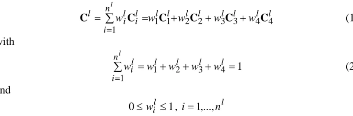
The problem of selecting a suitable material has been investigated for a long time. It has found a natural application in the optimal distribution of fiber orientations in composite structures [1-3] and in the identification of the optimal stacking sequence (see [4-8] amongst many others). In most practical applications, the candidate materials are restricted to 0, 45, -45 and 90° plies, which are the conventional orientations used in aeronautics. In their recent work, Lund and co-workers [9-14] have proposed the Discrete Material Optimization (DMO) approach to parameterize the topology optimization problem of structures made of fibers reinforced composite materials. This approach is an extension of the multi-phase topology optimization proposed in [15]. When applied to a composite ply denoted as l, it consists in writing the linear anisotropic material stiffness matrix Cl as a weighted sum of the stiffness of some candidate materials. When conventional laminates are used, and assuming that materials 1, 2, 3 and 4 correspond to fibers oriented at 0°, 45°, 90° and -45°, respectively, the following applies (no summation over the index l):

l l l l l l l l n i l i l i l w w w w w l 4 4 3 3 2 2 1 1 1 C C C C C C        (1) with 1 4 3 2 1 1        l l l l n i l i w w w w w l (2) and 1 0w_il  , i1,...,nl

In (1) and (2), nl _{is equal to 4 since 4 candidate orientations are considered.}

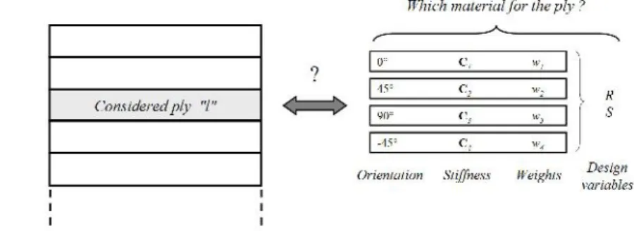
Equation (2) needs to be satisfied because it is a condition to obtain physically meaningful results. At the optimum, the physical ply l should be made of one (and only one) of the candidate plies, with the material properties C1, C2, C3 or C4 (Figure 1).

Figure 1. Identification of the optimal material for the ply in a DMO scheme

Several schemes have been proposed in [9-14] for defining the value of the weighting factors wi in (1). According to [12], the schemes of Equations (3) and

(4) are the most reliable ones. These are called DMO4 and DMO5, respectively, in [12]. Omitting the index l, they are written:

 



 



In (3) and (4), the parameters xi (i = 1,…,n) are the design variables, which take

their values between 0 and 1. According to those authors [9-14], the problem with DMO4 (3) is that the condition (2) is only verified for design variables xi equal to

0 or 1, which could lead to convergence problems; the difficulty with DMO5, which is a scaled version of DMO4, is that the effect of the penalization p is less predominant, and the results can be made of many intermediate densities. Nevertheless, both DMO4 and DMO5 perform well, and interesting solutions have been obtained in [9-14]. Finally, DMO is a very general method able to manage an arbitrary number of candidate materials.

2. New material parameterization

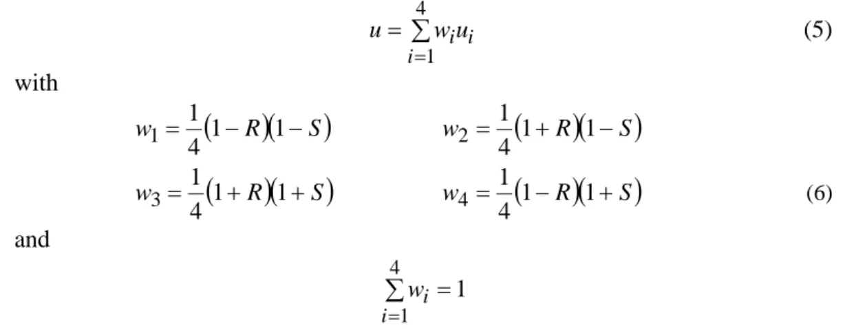
Referring to the finite element theory [16], Equation (2) represents the partition of unity, which is, by definition, satisfied by the shape functions, here denoted wi,

used to interpolate some nodal values ui. For instance, with a quadrangular first

order finite element, there are 4 nodes (vertices) noted i (i = 1,…,4) and the approximation of a field u is written as:

   4 1 i i i u w u (5) with

























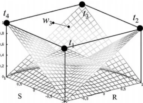
R and S are the natural coordinates representing the 2 parameters needed to define the shape functions of the reference quadrangular finite element (6). They take their values between -1 and +1 in the reference (integration) space (Figure 2a). Each vertex of the reference quadrangular element is characterized by a specific value, either +1 or -1, for R and S.

Based on these facts, a candidate material could be assigned to each vertex of the quadrangle, as illustrated in Figure 2b, identified by a couple of values (R;S). With this definition, the shape functions (SF) of (6) become the weights in the stiffness definition (1). They are illustrated in Figure 3. Two design variables, R and S, are then sufficient to identify a conventional ply from a set of -45, 0, 45 and 90° fiber orientations. In summary, the weights (6) take the following form, called the SF parameterization:







w_iSF  1 1 4

1

for SF (7)

Figure 3. Illustration of the weighting factors of the new material parameterization For example, if R = S = 1 at the solution, w3of (6) is equal to 1 and w1= w2= w4

= 0; when replaced in (1), it results that the optimal material is characterized by

the C3 constitutive matrix, and the corresponding ply is therefore made of fibers oriented at 90° (Figures 2 and 3). The assignment of the material properties to the vertices is of course not unique, however, it does not influence the results. The principle of the SF parameterization is illustrated in Figure 4.

Figure 4. Identification of the optimal material for the ply in an SF scheme

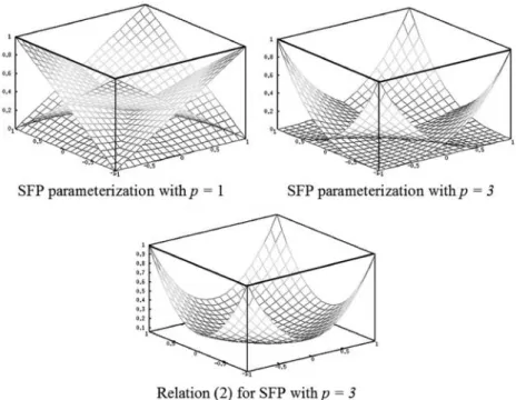
As depicted in Figure 3, the parameterization proposed in (7) does not penalize the intermediate values of the design variables R and S, since the shape functions are bilinear in R and S. As Equation (2) must at least be satisfied at the solution but not necessarily during the iteration history, we can therefore penalize weights in (7) with an exponent p in order to force the selection of only one material at the solution, thus limiting the occurrence of any blending of materials in a given physical ply at the optimum. The resulting SFP scheme (SF with penalization) is written like this:







When p is equal to 1, the SFP scheme is equivalent to the SF parameterization (7). The weighting coefficients are illustrated in Figure 5, for different values of the exponent p. When an exponent is used in the SF formulation, Equation (2) is no longer satisfied during the optimization process, especially for intermediate values of R and S (Figure 5). In this case, a resource constraint based on (2) could be

added in the problem. It will be shown in the numerical tests that such a constraint does not have to be considered in the problem when the value of p is large enough. This statement is valid for the compliance problems which are considered in this paper. This should be checked for other kinds of structural responses, such as buckling and local constraints.

Figure 5. Illustration of the weighting coefficients of the SFP parameterizations. Top: SF and SFP with p = 3. Bottom: sum over the wi(for p=3)

In Figure 6, it is seen that the proposed SFP parameterization with a penalty on the intermediate values of the design variables is very similar to the SIMP law classically used in topology optimization [17].

Figure 6. Illustration of SFP, with p = 1, 3 and 5, when only R varies (S = -1)

The advantage of the SFP approach is that only 2 design variables are needed to select a material in a set of 4 candidates. The size of the optimization problem is therefore halved when compared to the DMO schemes. In addition, the shape of the penalty functions illustrated in Figures 5 and 6 seems suitable to penalize the

intermediate values of the design variables. Despite the difference in the definition of the parameterizations (4) and (8), the sensitivity analysis proposed in [9-14] could be easily adapted to the SF and SFP definitions.

As it is the case for DMO4 with DMO5, a scaled version of SFP could be provided. However, the evolution of the resulting weighting coefficients is very similar to the one observed for the DMO5 scheme [12]. These scaled versions of SFP are not tested in this paper.

When a topology optimization problem is formulated, the ply can disappear at the solution. It is therefore necessary to include in the parameterization (8) an additional design variable  related to the classical SIMP formulation [17]. The material stiffness related to the ply l then becomes:

 

The value of q in (9) is not necessarily equal to p in (3) and (8).

The SFP method presented in this paper is less general than the DMO approach. SFP could certainly be extended to more (or less) than 4 materials, based on the existing finite element shape functions, with 2, 3 and 8 nodes (bar, triangle membrane, and hexagonal volume element, respectively). For 5, 6 and 7 candidate materials, shape functions with mixed degrees on the edges could be used. The definition of the shape functions mentioned above should be adapted in order to satisfy the non negativity constraint on the weights wi, which is a condition to

provide physical solutions. These extensions of SFP are not tested in this paper, which considers only 4 materials and aims primarily to present the first idea for an alternative to DMO.

The following numerical tests will focus on the ply selection in membrane problems. As shown in Figure 4, SFP could however be used for the stacking sequence optimization. In this case, specific design rules should be taken into account in the optimization problem. Such constraints should be defined on the weights wi. For example, the constraint requiring a minimum percentage of 0°

plies in the solution could be expressed based on a sum of the weights w1 of each

ply in the transverse direction. Other restrictions, such as no more than 4 consecutive plies with the same orientation, could also be defined. Such extensions are currently being investigated [18], but need further study.

As is the case for DMO, the solution provided by SFP will be sub-optimal. It is well known that when a discrete optimization problem is replaced by a continuous approach with a penalty to exclude intermediate values of the design variables, local optima appear in the design space [19], and the optimizer can become trapped in such local solutions. This occurs even when a continuation approach is used with a penalization technique [20].

3. Numerical test cases

Three numerical applications are solved in this paper. Despite being simple, they are sufficient to highlight the difficulties of the optimization problem, to enable an easy interpretation of the results and to appreciate the capabilities of the new parameterization scheme.

The objective is to select the best orientation of composite plies (0, -45, 45 or 90°), which maximizes the global in-plane structural stiffness, in a linear static analysis. The material properties are given in Table 1.

E11= 146860 MPa E22= 10620 MPa E33= 10620 MPa

12= 0.33 13= 0.33 23= 0.33

G12= 5450 MPa G13= 5450 MPa G23= 3990 MPa

Table 1. Material properties of the C12K/R6376 graphite epoxy

Our own implementation of MMA [21,22], available in the BOSS Quattro optimization tool box [23], is used. The structural analysis is conducted with the SAMCEF finite element code [24]. The sensitivity analysis is carried out by finite differences.

Three parameterization schemes are compared: DMO4, DMO5 and SFP. For the DMO4 and DMO5 schemes, as expressed in (3) and (4) and illustrated in Figure 1, four design variables xiare needed for each physical ply. For DMO4, a resource

constraint could be considered, defined either by (10) or (11). Those 2 constraints are however not added to the optimization problem, but are computed in order to check whether the obtained solution is – in some sense – physically meaningful.

1 4 1 





For the SFP scheme (8), 2 design variables are sufficient in each physical ply, as illustrated in Figure 4, and the constraint (10) could be included in the optimization problem (although it is not the case in this paper). Different values of

p in (8) are tested.

The starting point for the optimization consists in an equal mix of the 4 candidate materials in each ply, i.e. xi = 0.25 (i = 1,…,4) for DMO4 and DMO5, while R =

S = 0 for SF and SFP. The same convergence criterion is used for all the tests: the

iterative process is stopped when the variation of the objective function between two iterations is less than 0.01%.

Structures submitted to in-plane loading are considered. For the convenience with the finite element code used here, the weighting factors wi are not applied to the

constitutive matrix Cl, but rather to the ply thickness tl of each candidate ply l. The approach then aims at determining the value of the thickness of the candidate

plies with fibers oriented at 0, -45, 45 and 90°, instead of selecting the corresponding constitutive matrix (Figure 7). Equation (2) initially applied to the material properties (1) is then converted to the restriction to have a complete ply thickness at the solution (no summation over the index l):

total l l l l l l l l n i l i l i l _{wt wt w t wt w t t} t l        1 11 22 33 44 (12)

In the applications, each physical ply should have a thickness equal to unity at the solution, that is ttotal = 1.0. As explained before, such a constraint (12) is not

added to the optimization problem, but computed anyway to check the obtained results.

Figure 7. Illustration of the weighting factors in SFP applied to the thickness of the candidate plies

3.1 First application : orientation of a single ply

In this first test case we consider a composite membrane clamped on one edge and subjected to a uniform traction on the opposite edge (Figure 8). The model is constituted of 16×16 first-order quadrangular membrane finite elements. The structure is made of one laminate including only one ply, and all the finite elements of the model will have the same fiber orientation at the solution. This ply is composed of 4 candidate materials, with fibers oriented at –45, 0, 45 and 90°. The optimization problem then includes 4 design variables for the DMO parameterizations, and 2 for the SFP ones.

The results are provided in Table 2. According to the load case (Figure 8), the optimal orientation is equal to 0°: t0° should therefore be equal to 1.0 at the optimum, while the other candidate ply thicknesses should vanish. These conditions are satisfied by the 7 configurations tested (Table 2).

Scheme DMO4 (p=5) DMO5 (p=5) SFP (p=1) SFP (p=1.5) SFP (p=2) SFP (p=3) SFP (p=5) Status Optimum reached Optimum reached Optimum reached Optimum reached Optimum reached Optimum reached Optimum reached Iterations 5 3 4 4 4 4 4

Table 2. Results of the test case of Figure 8 and status of the solution

The same problem is now solved with a load acting in a vertical direction, as illustrated in Figure 9. In this case, the optimal solution is given by a ply oriented at -45°.

Figure 9. First test case: vertical load

In Table 3, the number of iterations needed to reach a solution is provided. It can be seen that the DMO4 and DMO5 schemes are not able to find the optimal solution. For DMO4 and DMO5, a blending of 0°, 90° and -45° plies is obtained; for DMO4 the resulting ply thickness is equal to 0.45 instead of 1.0. The optimum is obtained for the SFP schemes when the exponent p is larger than or equal to 2. In this case, a thickness equal to 1.0 is obtained after 4 iterations. For lower values of the exponent, a blending of either the 4 candidate materials, or 0° and -45° plies is obtained. Moreover, for SFP with p = 1.5, the total thickness at the solution is equal to 0.7 instead of 1.0. In conclusion, SFP reaches the optimal solution consisting of a unique ply at -45° when the value of the exponent p is larger than or equal to 2. DMO is unable to identify this optimum.

Scheme DMO4 (p=5) DMO5 (p=5) SF (p=1) SFP (p=1.5) SFP (p=2) SFP (p=3) SFP (p=5) Status Optimum not reached Optimum not reached Optimum not reached Optimum not reached Optimum reached Optimum reached Optimum reached Iterations 26 38 19 17 4 4 4

3.2 Second application : non homogeneous composite

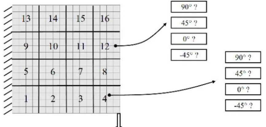
The problem of Figure 10 is considered. The structure is divided into 16 regions of independent fiber orientations. In each region, we are looking for the best ply amongst the set of 0, 45, 90 and -45° orientations. The orientations can therefore vary from region to region at the solution. For the DMO schemes, 64 design variables are needed. For the SFP parameterizations, 32 design variables are used.

Figure 10. Second test case: vertical load and non homogeneous laminate. Numbering of the regions

The results are presented in Table 4. For the DMO4 scheme, a blending of orientations is present at the solution and the total thickness is not equal to 1.0, in the regions 8, 12, 15 and 16 of Figure 10. For DMO5, the pattern obtained at the convergence is illustrated in Figure 11. At iteration 4, a smaller value of the objective function was obtained (very close to the one obtained with SFP and p ≥

2), but for a pattern including a blending (95% versus 5%) of materials in 10

regions. The underlying solution with the material covering 95% is the same as the one obtained for SFP with p ≥ 2. For the SFP schemes with an exponent p larger than or equal to 2 the solution of Figure 11 is obtained in 4 iterations, and the thickness is equal to 1.0 at the optimum. For SFP with p = 1.5, a blending of plies is present in 3 regions. For SFP with p = 1, no meaningful solution is obtained. In conclusion, SFP reaches a solution representing the smallest value of the objective function and no blending of plies in each region when p is larger than or equal to 2. DMO4 provides a solution with blending of plies. DMO5 provides a solution without blending of plies but with a higher value of the objective function in comparison to SFP.

Scheme DMO4 (p=5) DMO5 (p=5) SFP (p=1) SFP (p=1.5) SFP (p=2) SFP (p=3) SFP (p=5) Status Blending of plies; Eq. (12) not satisfied No blending of plies; Larger OBJ Blending of plies Blending of plies No blending of plies; lowest OBJ No blending of plies; lowest OBJ No blending of plies; lowest OBJ Iterations 18 5 15 18 4 4 4

Table 4. Results of the test case of Figure 10. OBJ stands for “objective function”

Figure 11. Orientations obtained with DMO5 and SFP (p = 2, 3 and 5)

3.3 Third application : topology optimization and material selection

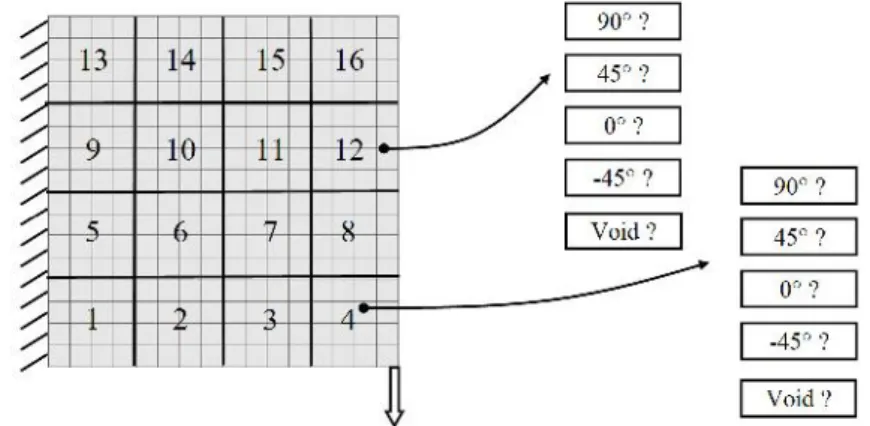
The additional design variables  introduced in (9) to remove material at the solution are used in this application. In the problem illustrated in Figure 12, 80 and 48 design variables are considered, for the DMO and SFP schemes, respectively. Removal of the material corresponding to 5 regions was imposed, which means that the global constraint (13) is added to the problem.

11 16 1 



In order to provide a “black and white” final design, the exponent q of (9) is equal to 6.

Figure 12. Third test case: vertical load and topology optimization

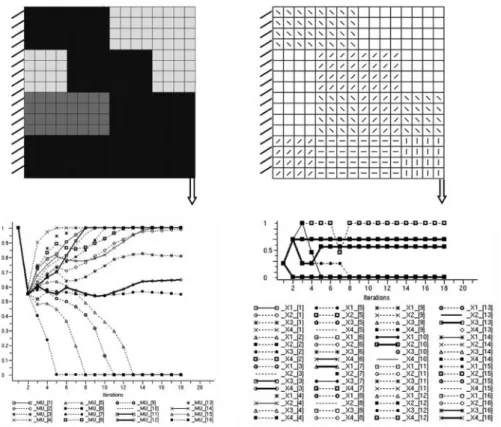
The results are presented in Table 5 and in Figures 13 and 14.

For the SFP scheme with p = 2, 3 and 5, the same orientations as shown in Figure 11 are obtained after 4 iterations. 15 additional steps are needed to identify the set of the optimal densities . For p = 1.5, a blending of materials is still present at the solution in region 14 of Figure 12, and some unexpected orientations are

present (e.g. -45° is obtained in region 13). For SFP with p = 1, the solution includes several regions with blended materials.

For DMO5, a solution is obtained after 18 iterations. This is illustrated in Figure 14. Small oscillations in the orientations appear during the iterative process. Moreover, their values are different to those obtained with the SFP approach. For the selected stopping criterion based on the objective function, some intermediate density variables  are still present at the solution. Even for a criterion based on the variation of the design variables between 2 iterations, some density variables kept their intermediate values. For DMO4, a blending of materials is observed in several regions, but the density design variables do not present intermediate values at the solution.

Finally, it is interesting to highlight that the overall speed of convergence is conditioned by the topology optimization problem associated with the density design variables. Scheme DMO4 (p=5) DMO5 (p=5) SFP (p=1) SFP (p=1.5) SFP (p=2) SFP (p=3) SFP (p=5)

Status Blending of plies Eq. (12) not satisfied No blending of plies; Larger OBJ Blending of plies Blending of plies No blending of plies; lowest OBJ No blending of plies; lowest OBJ No blending of plies; lowest OBJ Iterations 32 18 22 20 19 19 19

Figure 13. Solution obtained with SFP with p = 2, 3 and 5 and q = 6

Figure 14. Solution obtained with DMO5 (p=5)

5. Conclusions

A new parameterization for material optimization has been presented. It is based on the shape functions classically used in finite elements, and is applied to the selection of conventional fiber orientations (0, 45, 90 and -45°) in composite structures. Compared to other schemes like DMO (Discrete Material Optimization), the SFP scheme (Shape Functions with Penalization) requires a smaller number of design variables. The specific shape of the resulting penalty functions is very similar to the SIMP law for topology optimization, and SFP seems less likely to provide a blending of candidate materials at the solution. The SFP parameterization is simple to understand and easy to use. The proposed method showed interesting results when tested on simple representative problems. Other parameterization schemes based on the same principle could be identified and applied, for instance, to the selection of isotropic material or composite sub-laminates.

Acknowledgements

The author would like to thank the Walloon Region of Belgium and Skywin (Aerospace Cluster of Wallonia) for their financial support through the project VIRTUALCOMP.

References

1. Pedersen P. (1989). On optimal orientation of orthotropic materials. Structural Optimization, 1, pp. 101-106.

2. Pedersen P. (1991). On thickness and orientational design with orthotropic materials. Structural Optimization, 3, pp. 69-78.

3. Hammer V. (1997). Design of composite laminates with optimized stiffness, strength and damage properties. PhD Thesis, DCAMM Report S72, Technical University of Denmark.

4. Haftka R.T. (1992). Stacking sequence optimization for buckling of laminated plates by integer programming. AIAA J. 30(3), pp. 814-819.

5. Le Riche R., Haftka R.T. (1993). Optimization of laminate stacking sequence for buckling load maximization by genetic algorithm. AIAA J., 31(5), pp. 951-956.

6. Diaconu C. and Sekine H. (2004). Layup optimization for buckling of laminated composite shells with restricted layer angles, AIAA J., 42(10), pp. 2153-2163.

7. Kin C.C. and Lee Y.J. (2004). Stacking sequence optimization of laminated composite structures using h-genetic algorithm with local improvement. Composite Structures, 63 (3), pp. 339-345.

8. Liu D., Toropov V., Barton D. and Querin O. (2009). Two methodologies for stacking sequence optimization of laminated composite materials. Proceedings of the International Symposium on Computational Structural Engineering, Shangai, China, June 22-24, 2009.

9. Lund E. and Stegmann J. Structural optimization of composite shell structures using a discrete constitutive parameterization. XXI ICTAM, 15-21 August 2004, Warsaw, Poland.

10. Lund E. and Stegmann J. On structural optimization of composite shell structures using a discrete constitutive parameterization. Wind Energy, 8, pp. 109-124, 2004.

11. Lund E., Kühlmeier L. and Stegmann J. Buckling optimization of laminated hybrid composite shell structures using discrete material optimization. 6th World Congress on Structural and Multidisciplinary Optimization, Rio de Janeiro, 30 May – 3 June 2005, Brazil.

12. Stegmann J. Analysis and optimization of laminated composite shell structures. PhD Thesis, Aalborg University, Denmark, 2005.

13. Stegmann J. and Lund E. Discrete material optimization of general composite shell structure. International Journal for Numerical Methods in Engineering, 62, pp. 2009-2027, 2005.

14. Lund E. Buckling topology optimization of laminated multi-material composite shell structures, Composite Structures, 91, pp. 158-167, 2009.

15. Sigmund O. and Torquato S. Design of materials with extreme thermal expansion using a three-phase topology optimization method. Journal of the Mechanics and Physics of Solids, 48, pp. 461-498, 2000.

16. Zienkiewicz O.C. The finite element method. 3rd edition, McGraw-Hill, New York, 1977.

17. Bendsoe M.P. and Sigmund O. (2004). Topology optimization: theory, methods and applications. Springer-Verlag.

18. Bruyneel M., Grihon S., Sosonkina M. New approach for the stacking sequence optimization based on continuous topology optimization. 8th _{ASMO UK/ISSMO Conference on Engineering Optimization,}

London, 8-9 July 2010.

19. Fu J.F., Fenton R.G., Cleghorn W.L. A mixed integer-discrete-continuous programming method and its application to engineering design optimization. Engineering Optimization, 17, pp. 263-280, 1991.

20. Stolpe M., Svanberg K. On the trajectory of penalization methods for topology optimization. Structural & Multidisciplinary Optimization, 21, pp. 128-139, 2001.

21. Svanberg K. (1987). The method of moving asymptotes: a new method for structural optimization. Int. J. Num. Meth. E,gng., 24, pp. 359-373.

22. Bruyneel M. (2006) A general and effective approach for the optimal design of fiber reinforced composite structures. Composites Science & Technology, 66, pp. 1303-1314.

23. Radovcic Y. and Remouchamps A. BOSS Quattro: an open system for parametric design. Structural & Multidisciplinary Optimization, 23, pp. 140-152.