Daniel M. Dubois
*HEC Management School – University
of Liege, rue Louvrex, 14,
B-4000 Liège, Belgium
[email protected]Stig C. Holmberg
Department of Information
Technology-and Media, Mid Sweden University
SE-83125 OSTERSUND, Sweden
shbg @ieee.orgAbstract
This paper deals with a new version of a web-based software simulation tool MLD-STAR (Management Learning and Decision making – Simulation Tool with Anticipation and Re-tardation), for the numerical simulation of mathematical models of management systems. A new algorithm is presented to automatically compute the numerical values of the paramet-ers of models to be simulated. The main idea consists in generating successive sets of val-ues of the parameters of the model with a ran-dom number generator, and to use a selection criterion for accepting or rejecting the sets of values. This self-adapting parameters method is so based on a Darwinian process of selec-tion. Results of simulations with such self-ad-apting parameters are given in using the math-ematical model given in Dubois and Holmberg (2006).
1
Introduction
Multi-layered systems with delays between their different logical levels are found in many models of management systems.
Dubois and Holmberg (2006) have demonstrated that it is possible to extend such models in introducing some anticipatory factors and to simulate the behaviour of such systems by applying anticipatory modelling and computing.
Further, they have shown that longer delays tend to increase the instability of the system, with greater fluctuations as a consequence. An anticipation factor, though, may help to counteract those fluctuations.
The current solution, however, is too crude in several aspects.
First, the control parameters have to be manually set before the simulation run starts. Hence, in the case of a bad mix of parameter values the simulation may run out of control with one or more output values swiftly moving toward infinity.
* Centre for Hyperincursion and Anticipation in Ordered
Sys-tems (CHAOS), Institute of Mathematics, Grande Traverse 12, B-4000 Liège 1, Belgium
(http://www.ulg.ac.be/mathgen/CHAOS).
In other words, once the simulation has started, there is no way to improve less well-chosen parameter values. Further, with the current user interface, a manager, who is using the tool for training purpose, will not be able to make continuous observations, reflections, and decisions during the simulation run similar to those made during real management. Hence, the purpose of this work is to correct those two main shortcomings in the current solution. This will be achieved by implementing a mechanism for self-adapting parameters and by designing a user interface, which is adapted to a manager’s view.
2
The model of the management
sys-tem and the simulation algorithm
The mathematical model of the management system given in Dubois and Holmberg (2006) will be used to demonstrate the algorithm for computing the self-adapting parameters.With retardation and anticipation, the model is given by the following differential equations:
dP(t)/dt = [cR(t − τR) + eV(t) − d]P(t) (1a)
dR(t)/dt = f + [bV (t) − cP(t)]R(t) (1b) dV(t)/dt = [a − bR(t) − eP(t + τA)]V(t) (1c)
where τR and τA are the retardation and the anticipation
time shifts.
The simulation tool M2-STAR implementing this model was designed and built, from the following al-gorithm [Dubois and Holmberg, 2006]:
P(t+1)=P(t)+dt[cP(t)R(t−tau)+eP(t)V(t)−dP(t)] (2a) R(t+1)=R(t)+dt[f+bR(t)V(t)−cR(t)P(t)] (2b) V(t+1)=V(t)+dt[aV(t)−bV(t)R(t)−eV(t)P(t)]
−e(ant)V(t)(P(t+1)−P(t))
−[e(ant2)/2dt](V(t)(P(t+1)−2P(t)+P(t−1)) (2c)
with the model parameters, a, b, c, d, e, f, the first and second order anticipation parameters, ant and ant2, the
retardation (delay) parameter, tau, the interval of discrete time, dt, the number of time steps, maxsteps, and with the initial conditions, V0, R0, and P0.
The purpose of this software tool was to visualise the dynamics and to test the validity of the model.
3
The simulation tool MLD-STAR
A new user interface was designed in order to meet the following objective: a manager using the tool could use it as close as possible in the same manner as he or she is running a real organisation.This new computer based simulation tool1 was named MLD-STAR (Management Learning and Decision making – Simulation Tool with Anticipation and Retardation). Compared with the original tool M2-STAR, discussed by Dubois and Holmberg (2006) this new version implements the following additional features:
1. At each simulation step it is possible to change one or more of the parameters before continuing to the next step. Those are the initial values V0, R0, and P0, the decision parameters a, b, c, d, e, and f, and the system parameters dt, tau (retardation) and ant (anticipation). There are also two additional parameters Lim1 and Lim2 influencing the learning mechanism. In this way it becomes possible for a manager or other decision maker to run the model and to experiment with continuous decision-making and decision changes.
2. At each step it is possible to back the simulation one or more steps, make parameter changes, and make a new try with advancing the simulation one or more steps. In this way it becomes possible to correct the consequences of an initially bad mix of parameter values.
3. It is possible to zoom in and out on both the horizontal and vertical axis. This makes it possible to switch between overviews and detail examination of the system plot and to make maximal use of the plotting area.
4. It is possible to switch right and left on the horizontal axis and up and down on the vertical one.
5. Besides the graphical plot, current, min, and max values are displayed numerically for vision (V), research (R), and production (P) functions.
6. Current and max allowed simulation step is displayed numerically.
7. There is a control for choosing an initial set of parameter values.
8. There is a control for choosing an initial learning mode. P, for example, in this control indicates that learning is active for the production (P) function. With those new features added it becomes possible to interact with the model in a rather free way.
It will, for example, be possible to advance the simulation step by step and to analyse the result after each step. If it becomes evident that the system is 1 http://www.c8systems.com/ldm (with the Mozilla Firefox
browser)
developing in an unwanted way the parameters may be changed in order to direct the system toward its target.
In so doing, the decision parameters have direct impacts on the following logical levels:
a -> Vision (normative planning)
b -> Vision and Research (strategic planning) c -> Research and Production
d -> Production
e -> Vision and Production f -> Research
In the system display, those impacts are indicated in connection to the corresponding parameter caption.
The delay parameter (tau) is not a decision parameter in the same sense as the foregoing. It is more a system property, which can be changed only by a redesign of the entire system.
The anticipation parameter (ant) is in a way a behavioural parameter. It indicates how far into the future the organisation is looking in its visionary work.
The new algorithm dealing with the self-adapting parameters in simulation of management systems will be presented in section 5.
4 Testing the tool MLD-STAR
The tool can be run in two different ways or modes, i.e. management mode and self-adapting mode.
In the first mode, the person running the tool has the opportunity to change one or several of the parameters before each simulation step. In a way he or she is here running the model in a similar way as a manager is managing a real organisation.
The experience here is that it is very difficult to correct the situation once the trajectory has started to run out of limits.
In the self-adapting mode there is an algorithm that automatically change the parameters in order to keep them within limits. Even here, however, the manager can override the process and manually change the parameters in each step.
For testing purpose five test sets, which represent some typical situations, were constructed. With help of those, the following tests were run.
4.1 Production focusing
With the parameter setting a = 0, b = 0, c = 0, d = 0.1, e = 0, f = 0, ant = 0, tau = 0, dt = 1, maxsteps = 1000, V0 = 0.02, R0 = 0.04, and P0 = 3.6 we have an organisation only focusing on production and putting no resources into creation of visions and development. The situation may seem a bit unrealistic but is anyhow interesting from a learning point of view.
Despite how big the initial production may be, it will quickly go down to zero. However, if the manager (runner of the model) reacts swiftly and chooses another parameter setting, or changes the parameters manually, after just two or three simulation steps the production trajectory will change. The post change development of the system may be far from stable, but
it is rather easy to find a solution, which prevents the production to go down to zero.
Learning, on the other hand, will not work in this situation as the learning algorithm, in its current implementation, just prevents the production trajectory from going towards infinity.
The example may be simplistic but anyhow it gives a concrete demonstration of the importance of normative and strategic planning in the organisation. Further, it gives clear evidence that agility and anticipation are crucial properties in any organisation.
4.2 Research focusing
With the next setting a = 0.4, b = 0.299, c = 0.21, d = 0.3, e = 0.1, f = 0.018, ant = 0, tau = 0, dt = 1, maxsteps = 1000, V0 = 0.4, R0 = 1.2, and P0 = 0.6 we have an organisation putting efforts on research but neglecting normative planning and vision creation. There is also no effort to transform research efforts into production.
There will be dumping oscillations but research is all the time the dominant output from the system. Vision and production will all the time be zero or close to zero. Even this example may seem unrealistic, but according to Cringely [1996] this is exactly what happened within the big company responsible for the research and development igniting the whole PC-technology and its industry.
By increasing the retardation to 2 or 4 the system will become more coupled. Hence, after each top in the research there will be a very short production peak.
Changing the retardation to 1 and setting p to 0 will have an interesting effect. Here the production will raise steadily the first 375 steps. After that there will be a short period of small oscillations before the production falls directly to zero. The production will not recover during the rest of the simulation run.
4.3 Both Vision and Research
With the parameter setting a = 0.2, b = 0.2, c = 0.2, d = 0.1, e = 0.2, f = 0.02, ant = 0, tau = 0, dt = 1, maxsteps = 1000, V0 = 0.6, R0 = 0.8, and P0 = 0.2 we are putting equal stress on vision (normative planning) and research (strategic planning).
The curves are oscillating but with anticipation set to 1 or 2 the oscillations will attenuate with higher simulation steps.
4.4 Anticipation and Delay
In this example, with the parameters set to a = 0.04, b = 0.02, c = 0.04, d = 0.064, e = 0.06, f = 0.004, ant = 0, tau = 0, dt = 1, maxteps = 1000, V0 = 0.6, R0 = 0.5, and P0 = 0.4, the delay effects become extra obvious. In each cycle the vision curve is the first to reach its maximum, after that follows the research curve and at last comes the production one. Further in each successive cycle the amplitudes increase slightly.
First, by increasing the retardation factor (tau) to 8 and 12 it becomes possible to see that the amplitudes will increase. So will also do the phase delays between the three curves.
Anticipation will here have a stabilising effect, which may be observed by in steps increasing ant from 1 to 12.
4.5 Chaos and Anticipation
At last, with parameters set to a = 0.21, b = 0.114, c = 0.33, d = 0.31, e = 0.118, f = 0.03, ant = 0, tau = 0, dt = 1, maxsteps = 1000, V0 = 0.6, R0 = 0.4, and P0 = 0.2 we will receive a chaotic outcome. By increasing the value of tau that behaviour will be further strengthened.
However, just by setting the anticipation value to a small value like 1 or 2 the system will quickly stabilise to a constant outcome. Further, changing of a parameter, for example f or d after 200 steps, will cause just a minor disturbance in the output. After a small jump the output curves will stabilise on new values close to the old ones. Hence, this is a nice example of the power of anticipation.
By increasing the retardation value tau to, for example 4, the system becomes more difficult to stabilise. Anyhow, by increasing the anticipation in steps from 1 to 20, the system becomes more stable in each step.
At last, by keeping the retardation value to 0 and setting anticipation to 6 or 7 some surprising patterns will emerge. This indicating that much remains to explore in multi layered management systems with anticipation and retardation.
The next section deals with the simulation of models in management systems with self-adapting parameters.
5 Mathematical development of a
Darwinian generator of the
self-adapting parameters
In Dubois and Holmberg (2006) the parameters a, b, c, d, e, f, were manually fixed before the simulation run was started and they did not change during the steps of the simulation.
An approach to self-adaptation could be inspired by the well-proven learning mechanisms already applied in Artificial Neural Networks (Chen, 1996). With such a learning approach the control parameters could automatically adjust themselves during the simulation run. The result would be a stable system, even in the case that the start values are less well chosen.
But we think that the first problem to resolve is the setting of the values of the parameters before running the simulation.
So, in this section, we will present an algorithm inspired by the Darwinian selection method and genetic algorithms for automatically computing the parameters of the model.
We will show that the Production (P), Research (R) and Vision (V) can be simulated in starting with such self-adapting parameters.
Indeed, the parameters will be now computed with a self-adapting method based on a Darwinian process of selection.
The main idea consists in generating successive sets of values of the parameters of the model with a random number generator, and to use selection criteria for accepting or rejecting the sets of values.
The criteria will be based on the stability of solu-tions with a set of parameters.
For that, the mathematical model equations (1abc) will be linearized.
5.1 Linearization of the non-linear model
The first step consists in determining the stationary solutions of eqs. 1abc in taking
dP(t)/dt = [cR(t − τR) + eV(t) − d]P(t) = 0 (3a)
dR(t)/dt = f + [bV(t) − cP(t)]R(t) = 0 (3b) dV(t)/dt = [a − bR(t) − eP(t + τA)]V(t) = 0 (3c)
The non-trivial stationary states are given by
P0 = a/e – bf/(ac – bd) (4a)
R0 = ef/(ac – bd) (4b)
V0 = d/e – cf/(ac – bd) (4c)
Let us define the new linearization variables, p(t), r(t) and v(t), from these stationary states by
P(t) = P0 + p(t) (5a)
R(t) = R0 + r(t) (5b)
V(t) = V0 + v(t) (5c)
Introducing these variables (5abc) in eqs. (1abc), after linearization, the following linear differential equations are obtained:
dp(t)/dt = P0[cr(t − τR) + ev(t)] (6a)
dr(t)/dt = R0[bv(t) − cp(t)] – [(ac – bd)/e]r(t) (6b)
dv(t)/dt = – V0[br(t) + ep(t + τA)] (6c)
With these three linear equations (6abc), we can obtain the criteria of local stability of the stationary solutions.
The criteria of stability will be given for the linear differential equations 6abc, without the retardation time shift, τR = 0, and without the anticipation time
shift, τA = 0. The purpose is to show that the
self-adapting parameters generation method is feasible.
5.2 Routh-Hurwitz criteria of stability
The criteria of local stability can be obtained in us-ing the well-known Routh-Hurwitz criteria.
From the characteristic equation for a third order system
λ3 + λ2a
1 + λa2 + a3 = 0 (7)
the local stability criteria are given by
a1 > 0 (7a)
a3 > 0 (7b)
a1a2 > a3 (7c)
After some mathematical developments, we have obtained the following characteristic equation for the linear system eqs. (6abc):
λ3 + λ2[(ac – bd)/e] + λ[bR
0bV0 + cP0cR0 + eP0eV0] +
[eP0V0(ac – bd)] = 0 (8)
with τR = 0, τA = 0.
So, the local stability conditions are given by
(ac – bd)/e > 0 (8a)
eP0V0(ac – bd) > 0 (8b) and [(ac – bd)/e] [bR0bV0 + cP0cR0 + eP0eV0] > [eP0V0(ac – bd)] or [bR0bV0 + cP0cR0 ] > 0 (8c)
The non-trivial stationary states 4abc must be positive for a viable management system:
P0 = a/e – bf/(ac – bd) > 0 (9a)
R0 = ef/(ac – bd) > 0 (9b)
V0 = d/e – cf/(ac – bd) > 0 (9c)
With the positive parameters:
a > 0, b > 0, c > 0, d > 0, e> 0 and f > 0 (10) the conditions for local stability are given by the conditions (9abc) that the stationary states are positive.
Indeed, from 9b, (ac – bd) > 0, the conditions (8a) and (8b) are fulfilled, and, the condition (8c) is fulfilled, because b >0, c > 0, R0 > 0, V0 > 0, P0 > 0.
5.3 Algorithm of the Darwinian genera-tor of self-adapting parameters
The algorithm for computing the parameters that give a local stability is based on the following method.
For all the positive parameters a > 0, b > 0, c > 0, d > 0, e> 0, f > 0
upper and lower intervals of values are defined: amax > a > amin, bmax > b > bmin, cmax > c > cmin,
dmax > d > dmin, emax > e > emin and fmax > f > fmin.
For the three positive stationary states: P0 > 0, R0 > 0, V0 > 0
upper and lower limits of values are also defined: PMAX > P0 > PMIN, RMAX > R0 > RMIN and
A random number generator generates successively sets of values for each parameter within the upper and lower limits:
amax > a > amin, bmax > b > bmin, cmax > c > cmin,
dmax > d > dmin, emax > e > emin and fmax > f > fmin.
Each set of the generated values of the parameters a, b, c, d, e, f
is used to compute the stationary states (4abc): P0 = a/e – bf/(ac – bd)
R0 = ef/(ac – bd)
V0 = d/e – cf/(ac – bd)
The set is accepted if the conditions PMAX > P0 > PMIN, RMAX > R0 > RMIN and
VMAX > V0 > VMIN
are fulfilled, otherwise, the set is rejected, and a new set of values of the parameters is generated randomly.
When the set of parameters is accepted, the simula-tion can begin.
Let us notice that the initial conditions P(0), R(0) and V(0) are also to be defined for running the simula-tion.
6 Simulation of the management
sys-tem model with the self-adapting
parameters
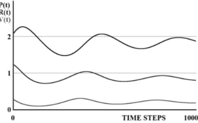
This section deals with the results of the simulation of the algorithm (eqs. 2abc) of the model (1abc), with the Darwinian method for computing the self-adapting parameters.
The simulations are made without anticipation ant = 0 and ant2 = 0,
and without retardation tau = 0.
The number of time steps of the simulation is equal to 1000, with the interval of time, d t= 1.
The lower and upper limits for the parameters: a, b, c, d, e, f
are chosen between 0 and 0.05.
The TABLES 1a, 1b and 1c, give the values of the fixed and self-adapted parameters of the algorithm for the 4 simulations given in Figures 1, 2, 3 and 4.
Table 1a: Minimum and maximum values of the stationary
states P0, R0 and V0, for the figures 1 to 4.
Figures PMIN PMAX RMIN RMAX VMIN VMAX
1 1.0 2.0 0.5 1.0 0.0 0.5
2 1.5 2.0 0.5 1.0 0.0 0.5
3 1.5 2.5 1.0 1.5 0.0 1.0
4 1.0 2.5 1.0 1.6 0.0 1.10
Table 1b: Continuation of the Table 1a. Values of the
meters (a, b, c, d, e, f) generated by the self-adapting para-meters Darwinian algorithm, for the figures 1 to 4.
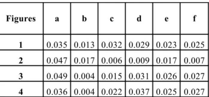
Figures a b c d e f
1 0.035 0.013 0.032 0.029 0.023 0.025 2 0.047 0.017 0.006 0.009 0.017 0.007 3 0.049 0.004 0.015 0.031 0.026 0.027 4 0.036 0.004 0.022 0.037 0.025 0.027
Table 1c: Continuation of the Table 1b. Values of the
sta-tionary states P0, R0 and V0, computed from the self-adapting
parameters, and the initial conditions P0, R0 and P0, for the figures 1 to 4. Figures P0 R0 V0 P0 R0 V0 1 1.092 0.753 0.224 1.3 1.1 0.6 2 1.875 0.853 0.226 2.1 1.2 0.3 3 1.702 1.190 0.504 2.1 1.3 0.8 4 1.275 1.034 0.559 0.3 0.2 0.1
Figure 1: Simulation of the management model with the
Figure 2: Simulation of the management model with the
self-adapting parameters.
Figure 3: Simulation of the management model with the
self-adapting parameters.
Figure 4: Simulation of the management model with the
self-adapting parameters.
We have thus demonstrated that this Darwinian method works with a great efficiency.
So, this Darwinian algorithm for generating self-adapting parameters will be implemented in the tool MLD-STAR.
7
Conclusions
This simulation tool may be seen as a clear demonstration of the Klir [1991] observation that the computer is the system researcher’s laboratory.
With help of MLD-STAR the theory for retardation in multi layered management systems and the accompanying formulas become living. The effects of different parameter combinations become obvious and the outcome may be studied in detail.
Further, it may be clarifying and learning to discuss the relation between model outcomes and the corresponding phenomena in real organisations. In experimenting with the tool many surprising patterns emerge. By reflecting on those new insights will surface. Those, in their turn, will trigger ideas for new parameter settings and experiments, and so on. In short, the tool may serve as a vehicle for learning and reflection.
At last, by experimenting with MLD-STAR new ideas are continuously born both concerning further development of the theory for anticipation and retardation in multi layered systems and further improvement of the simulation tool itself. Hence, theory building, model building, and experimenting seem to be a generic mix for scientific effectiveness.
References
[Chen, 1996] C. H. Chen, editor. Fuzzy Logic and
Neural Network Handbook. McGraw-Hill, New
York, 1996.
[Cringely, 1996] Robert X. Cringely. Accidental
Empires. Harper Business, New York, Paperback,
1996.
[Dubois, 2003] Daniel M. Dubois. Mathematical foundations of discrete and functional systems with strong and weak anticipations. In Martin Butz et. al., editors. Anticipatory Behavior in Adaptive Learning
Systems, State-of-the-Art Survey, Lecture Notes in
Artificial Intelligence, Springer LNAI 2684. (2003) 110—132, Berlin, 2003.
[Dubois and Holmberg, 2006] Daniel M. Dubois and Stig C. Holmberg. The Paradigm of Anticipation in Systemic Management. In Robert Trappl, editor.
Cybernetics and Systems 2006, Vol. 1, pp 15 – 20,
Austrian Society for Cybernetic Studies, Vienna, 2006.
[Fishwick, 2007] Paul A. Fichwick, editor. Handbook
of Dynamic System Modeling. Chapman &
Hall/CRC, London, 2007.
[Holmberg, 1999] Stig C. Holmberg. Multimodal Systemic Anticipation. I. J. of Computing
Anticipatory Systems, Vol. 3. Pp 75—84, 1999.
[Klir, 1991] George J. Klir. Facets of Systems Science. Plenum Press, New York, 1991.
[Schwaninger, 2000] Markus Schwaninger. Managing Complexity - The Path Toward Intelligent Organiza-tions. Systems Practice and Actions Research, Vol. 13:2. pp 207—241, 2000