Modelling and Simulating Complex Systems in Biology: introducing NetBioDyn

HAL Id: hal-01407520

https://hal.archives-ouvertes.fr/hal-01407520

HAL is a multi-disciplinary open access archive for the deposit and dissemination of sci-entific research documents, whether they are pub-lished or not. The documents may come from teaching and research institutions in France or abroad, or from public or private research centers.

L’archive ouverte pluridisciplinaire HAL, est destinée au dépôt et à la diffusion de documents scientifiques de niveau recherche, publiés ou non, émanant des établissements d’enseignement et de recherche français ou étrangers, des laboratoires publics ou privés.

Modelling and Simulating Complex Systems in Biology:

introducing NetBioDyn

Pascal Ballet, Jérémy Rivière, Alain Pothet, Michaël Théron, Karine

Pichavant, Frank Abautret, Alexandra Fronville, Vincent Rodin

To cite this version:

Pascal Ballet, Jérémy Rivière, Alain Pothet, Michaël Théron, Karine Pichavant, et al.. Modelling and Simulating Complex Systems in Biology: introducing NetBioDyn : A Pedagogical and Intuitive Agent-Based Software. Multi-Agent-Agent-Based Simulations Applied to Biological and Environmental Systems, IGI Global, 2017, 978-1-5225-1756-6. �10.4018/978-1-5225-1756-6.ch006�. �hal-01407520�

In book “Multi-Agent-Based Simulations Applied to Biological and Environmental Systems”, Chapter 6, pages 128-158, 2017.

DRAFT VERSION

Modelling and Simulating

Complex Systems in Biology:

Introducing NetBioDyn – A Pedagogical

and Intuitive Agent-Based Software

Pascal Ballet, LaTIM, INSERM, UMR 1101, Université de Bretagne Occidentale, France Jérémy Rivière, Lab-STICC, CNRS, UMR 6285, Université de Bretagne Occidentale, France Alain Pothet, Académie de Créteil, France

Michaël Theron, ORPHY, EA 4324, Université de Bretagne Occidentale, France Karine Pichavant, ORPHY, EA 4324, Université de Bretagne Occidentale, France Frank Abautret, Collège Max Jacob, France

Alexandra Fronville, LaTIM, INSERM, UMR 1101, Université de Bretagne Occidentale, France Vincent Rodin, Lab-STICC, CNRS, UMR 6285, Université de Bretagne Occidentale, France

ABSTRACT

Modelling and teaching complex biological systems is a difficult process. Multi-Agent Based Simulations (MABS) have proved to be an appropriate approach both in research and education when dealing with such systems including emergent, self-organizing phenomena. This chapter presents NetBioDyn, an original software aimed at biologists (students, teachers, researchers) to easily build and simulate complex biological mechanisms observed in multicellular and molecular systems. Thanks to its specific graphical user interface guided by the multi-agent paradigm, this software does not need any prerequisite in computer programming. It thus allows users to create in a simple way bottom-up models where unexpected behaviours can emerge from many interacting entities. This multi-platform software has been used in middle schools, high schools and universities since 2010. A qualitative survey is also presented, showing its ability to adapt to a wide and heterogeneous audience. The Java executable and the source code are available online at

1. INTRODUCTION

The theory of complex systems has become more and more relevant over the last thirty years to understand concepts such as emergence and self-organization and their role in biological, physical, chemical and social systems (Jacobson & Wilensky, 2006). Modelling and simulating these concepts behind the theory of complex systems is now very important, especially for biologists (students, teachers, researchers). For example, recent works have highlighted the complementarity of modelling both bottom-up and top-down (aggregated) approaches (Stroup & Wilensky, 2014). It has been shown though that teaching and learning complex systems are challenging tasks, and raise a lot of pedagogical issues. The two main issues are:

1. A widely taught top-down approach that have led students to think in that unique way; and 2. System dynamics that are difficult to understand and can be non-linear and

counter-intuitive (Jacobson & Wilensky, 2006).

Among different strategies, the use of Multi-Agent Based Simulations (MABS) in research, teaching and learning has proved to be an efficient way of answering (some of) these issues (Epstein, 1999; Jacobson & Wilensky, 2006; Ginovart, 2014). Indeed, the individual-based approach, in opposition to a population-based approach (such as ordinary differential equations), focuses on the entities of the system, their behaviour and their local interactions to explain the global system's behaviour. As such, this concept is easier to understand, more intuitive and do not require advanced mathematical skills (Ginovart, 2014). The use of computer tools to implement these models in virtual environments and simulate them allows researchers and students to generate hypothesis, test them and, especially for students, build their knowledge more efficiently (in a process of abduction (Houser, 1992)), see Section 2.2). NetLogo (Wilensky, 1999) is a good example of such agent-based software, and has been used in a lot of works, both in education (Gammack, 2015) and research (Banitz, Gras, & Ginovart, 2015).

This chapter focuses on how to teach complex biological systems to, for example, university students in Biology, middle school and high school students; students who often do not have any experience in computer programming, and/or are reluctant to implement any code. The problem is that most of agent-based software require knowledge and skills in programming languages such as Java (e.g. the Repast software (North, Collier, & Vos, 2006)) or the NetLogo environment. This is an issue that occurs more and more as the use of agent-based software, both in research and teaching, grows in social and life sciences. In (Ginovart, 2014) and (Gkiolmas, Karamanos, Chalkidis, Skordoulis, & Papaconstantinou, 2013), a model of a predator-prey system is used with NetLogo to help respectively first-year and high-school students to understand individual-based approaches and eco-systemic mechanisms. Despite its interest, this model is a ready-made one, coded in NetLogo, where the students can change some parameters of the simulation, but are not implied in the process of creating their own simulation from scratch. Indeed, implementing this model is considered as “a hard task” by the students (Ginovart, 2014) and could be counterproductive: looking for errors in the code instead of thinking at the rightness of the model. The authors argue that using pre-existent models could have a part in preventing students for building their own system's

representation (this point will be developed in Section 2.2). The gap between most of

agent-based software prerequisites and the actual programming skills of students (and sometimes researchers) in these fields has to be dramatically reduced and the processes of implementing a model and simulate it should be more intuitive.

This chapter essentially looks at the modelling of biological systems at and around the cellular scale. However, it is interesting to note that a lot of works have been focusing on modelling and simulating systems at the molecular scale, resulting in several software developed for students. For example, it is possible to find molecular visualisation systems like PyMol (Schrödinger, 2015) or software that help the docking of molecules like AutoDock Vina (Trott & Olson, 2010). There is also an automatic plotting of protein-ligand interactions with Lig-Plot (Wallace, Laskowski, & Thornton, 1996). It is possible to visualise molecular interaction networks and biological pathways thanks to software like CytoScape (Shannon et al., 2003). When focusing on DNA, a complete suite in Python can be used for the sequence alignment (BioPython - Cock et al., 2009). All these software are sources of inspiration when dealing at the cellular level.

In this chapter, the authors propose a software called NetBioDyn working like a game construction kit, where entities are located in a 3D grid environment and follow simple local transformation rules. In the name NetBioDyn, Bio stands for Biology, Dyn for Dynamic and Net comes from Internet because initially NetBioDyn was a Java Applet. Though this software is dedicated to cellular systems where several cells are in interaction, it can also model and simulate molecular mechanisms in a simple and symbolic way. The process of building models and simulations is facilitated by a graphical user interface similar to a drawing software like Microsoft® Paint. Researchers or students can build their own models, continuously visualize a clear representation of these models, and see them evolving in time and space. The results are displayed like a chess board with moving and changing coloured entities and can be analysed thanks to recorded population curves. From the point of view of the researcher (who usually is a teacher too), the software can help to explain non-intuitive and complex biological systems in a visual way, easily understandable by his peers or students. The authors present in this chapter the key principles of the software in rigorous but comprehensive language and develop three examples coming from real biological systems. The first example is a predator-prey system involving two bacteria. The second one simulates the mechanism of oxygen exchange in the zebra fish gills between water and blood. The third one simulates the blood coagulation mechanisms in a small section of a vein. A discussion is then engaged to show the interests of such software as well as the limits and drawbacks. A qualitative survey is also presented to show how students in biology and students in computer sciences have received the software. After the conclusion, different perspectives are presented in order to improve both the software and its use.

2. BACKGROUND

The use of computers in teaching biology can be divided into three common practices:

1. The development of models and simulations using a programming language like C++, Python or Java. This practice is powerful but takes time and requires advanced programming skills.

2. The use of customizable software, where students work on pre-existent models and can only change some parameters in simulations. This approach is very easy to use with students, but is not as efficient as building their own models.

3. The use of modelling software to help students develop their own models without any programming skills.

This third practice requires though the development of complex software that simplifies the process of modelling, by proposing for example, a graphical representation and construction of virtual agents, their behaviours and their environment.

Naturally, these three practices can also be found in the use of Multi-Agent Based Simulations and agent-based software in teaching biology. A quick overview of:

1. Agent-based modelling software that allow the development of models and simulations thanks to a programming language,

2. Agent-based modelling software that propose pre-made simulations, or 3. Computer aided-design modelling software is presented here.

A more complete review of agent-based environments has been made by Nikolai and Madey (2009), where more than 50 platforms are classified and discussed. Readers who wish to deepen the potential of the multi-agent approach for the simulation of complex systems can refer to the book edited by Weiss (2000), especially the chapter “Search Algorithms for Agents”.

2.1. Agent-Based Software in Biology Programming Languages

NetLogo (Wilensky, 1999) is one of the most well-known software allowing the development of agent-based programs, including simulations. It has a simplified programming language and simple mechanisms to create interfaces. This software is widely used in the community of biologists and many biological systems have been developed thanks to it. It has also been specifically used to help students understand the mechanisms behind complex systems (Stroup, 2014, Jacobson & Wilensky 2006). Nevertheless, pupils or students have to learn a programming language if they want to create their own models (Ginovart, 2014, Gkiolmas et al., 2013). One can also mention AgentSheets (Repenning, & Sumner, 1995) and AgentCubes (Repenning, Smith, Owen, & Repenning, 2012), which are simple programming environments allowing middle school pupils to learn programming in an appealing manner. These software are designed for multi-purpose applications and mostly games. They are based on a multi-agent system where behaviours are created by drag and drop condition-action algorithms. Although the programming is easy, some code is still required. Among generic multi-agent platforms, one can cite Breve (Klein, 2014; Klein & Spector, 2009) and Repast (North et al., 2006). Despite the fact that they have integrated development environments, the creation of models and simulations needs the knowledge of a programming language like Python, Groovy or Java. More recently, Biocellion (Kang, Kahan, McDermott, Flann, & Shmulevich, 2014) allows accelerating discrete agent-based simulation of biological systems with millions to trillions of cells. It uses cluster computers by partitioning the work to run on multiple compute nodes. It requires though mathematical modelling backgrounds and C++ programming skills.

Pre-Maid Simulations

Different simulations of multi-agent systems have been developed with NetLogo. The community models website of NetLogo proposes, for example, a customizable simulation of a predator - prey - poison system with 11 parameters: initial number rabbits and coyotes, rabbit reproducing probability, grass regrowth time, poison quantity, etc. (Jenkins, 2015). Concerning the simulation of multicellular systems, one can cite VirtualLeaf (Merks, Guravage, Inzé, & Beemstaer, 2001) which allows the simulation of tree-like structures based on agent representing cells and regulation network. It includes 12 different models and about

60 parameters that can be adjusted (e.g. cell mechanic or mathematical integration parameters).

Computer Aided-Design Software

In addition to a simplified programming language, NetLogo provides a “System Dynamic Modeler” that can be used to represent the dynamic of the system, entities inter-relations, feedback loops, flows and stocks. However, this tool requires a global understanding of the system (that is often missing with an agent-based approach) and is quite difficult to use as an intuitive modelling tool. Ioda (Interaction-Oriented Design of Agent simulations) and Jedi (an implementation of the Ioda concepts), allow the creation of multi-agent simulations in a very simple manner (without any coding skill), where predefined interactions can be added between agents (Kubera, Mathieu, & Picault, 2008). As Jedi is a demonstration software, it cannot be used to create complex simulations (4 agents maximum can be manipulated at the same time and there is no graphical user interface to precisely build the initial state). AnyLogic (XJ Technologies Company Ltd., 2012) is a multipurpose simulation software with a visual development environment. It has pre-built object libraries allowing users to create models by a drag-and-drop of elements. Its generic architecture makes it a powerful software but it could be relatively complex to understand for some students, especially the secondary ones. Another very interesting human-computer interaction is developed in the SimSketch software (Bollen, 2013). In this approach, the user draws the agents using an integrated paint tool then adds a name, a type and different pre-defined behaviours. This software focuses on primary and early secondary school students whereas this work focuses on the end of the secondary school to the university. Note that, this tool is not yet totally usable to create multicellular systems because there is no if...then...else structure. The software called CompuCell3D (Izaguirre et al., 2004) allows the simulation of multicellular systems with a user-friendly interface. The Python programming language can be used to create models but an XML file can also be edited to create simulations without coding. SimBioDyn (Ballet, Zemirline, & Marcé, 2004) is a software based on a hybrid multi-agent and mass-spring system designed to graphically create multicellular systems. Although rich in features (cell deformation, migration, adhesion and differentiation, molecular production and consumption and configurable through scripts in Python), it remains hard to use by non-specialists without a course of several hours (Ballet et al., 2004).

Among computer aided-design software, there are also some interesting works that have focused on modelling biological systems following other bottom-up or top-down approaches. For example, one can cite Virtual Cell (Shin, Liu, Loew, & Schaff, 1998), a software allowing to model intra-cellular mechanisms thanks to differential equations. It has a rich web-based Java interface to specify compartmental topology and geometry, molecular data and interaction parameters. However, the purpose of this software is to simulate a single whole cell or sub-parts of a cell but not multicellular systems, and it is not fitted for non-specialist users as advanced skills in mathematics are needed.

In this chapter, the authors focus on teaching pupils or students with no programming knowledge complex biological systems, such as multicellular systems.

In this context, the interests of using computer aided-design software are multiple :

 The student do not focus on how to program but on what to model (they remain in the field of biology).

 They cannot make syntactic or lexical errors: their models are always functional despite the fact that they can make semantic errors.

 They are no longer in charge of just some simulation parameters, but become the main actors of the model building, thus favouring the building of their knowledge.

 The teacher visualizes quickly where a student has insufficient knowledge.

So what is needed is a modelling software designed to be used by students with no programming knowledge and dedicated to agent-based multicellular systems modelling and simulation. However, this survey shows that many computer aided-design software exist, but to our knowledge none of them are intuitive enough to be used in this context. In order to answer these issues and give students the ability to easily create their own models, the authors have developed the software called NetBioDyn.

2.2. Reasoning About Complexity

Presenting essential concepts on system dynamics has become very important for students in biology. Teaching and reasoning about complex systems still raise a lot of pedagogical issues as shown in particular by Jacobson and Wilensky (2006).

Lynch and Ferguson (2014) argue that grasping the complexity requires a representational framework able both to describe executable computer models and to support reasoning as a simply readable “external representation”, as opposed to internal representations that are the user's mental models (Zhang and Patel, 2006). According to them, a good external representation affords the classic scientific approach, called abduction, emphasizing the observation, the build of hypothesis and the tests to verify the relevance of assumptions (Houser, 1992): it promotes the exploration and understanding of a phenomena thanks to a practical approach. It should be too constructed by the students themselves for two principal reasons: the first one is that it improves their learning (better memorization, quasi-physical experimentation of the model and appropriation of fundamental mechanisms) and the second one concerns the amelioration of their self-commitment (Prain, & Waldrip, 2006). Lynch and Ferguson define an ideal representation as “some written, external representation to complement user's internal representations [...], producing an external cognitive artefact which facilitates exploration and discovery [...] while also offering the ability to be executed”. Lynch and Ferguson summarize the 9 properties of a suitable external representation that were previously defined by Zhang and Patel (2006):

 Short-term or long-term memory aids.  Directly perceived information.

 Knowledge and skills that are unavailable internally.  Support for easy recognition and inference.

 Unconscious support for cognitive behaviour.  More efficient action sequences generated.

 Facilities to stop time and make information visible and sustainable.  Need for abstraction reduced.

 Aids to decision making through high accuracy and low effort.

Following these properties, the authors claim that NetBioDyn, thanks to its graphic interface and its simulation tools proposes a suitable external representation. It gives to students and teacher a simple way to create and experiment and test models of biological systems, while providing at any time a simplified and complete view of the system's state.

More generally, readers who want to improve their knowledge on “learning by doing” in virtual environments (VE) can read the book of Aldrich (2009).

3. NETBIODYN, A PEDAGOGICAL AND INTUITIVE AGENT-BASED SOFTWARE NetBioDyn is a fully open source Integrated Development Environment (IDE) dedicated to teaching activities in biological complex systems, mainly at the cellular level and secondarily at the molecular scale. It gives the possibility to teachers and students to create simulations of multicellular and multi-molecular systems in a simple and visual manner. NetBioDyn does not require any skill in computing and lays on the agent-based approach. Besides being simple to understand for students, this approach allowed the authors to design an intuitive graphical user interface to easily manipulate the agent-based concepts: entity, behaviour and interaction. In this section the graphical user interface of the software is first presented. Then, the section goes inside the software architecture with the description of the entities populating the simulated environment and how they can evolve thanks to algorithmic behaviours (movement, differentiation, division, apoptosis, etc.). In the next section, three examples of easily reproducible simulations are detailed. The code and the executable (for UNIX, Mac and Windows Operating Systems) are available for download on the website

http://virtulab.univ-brest.fr.

3.1. Graphical User Interface

For educational purpose, the design of a graphical user interface is a crucial point. For the student or the teacher who creates a simulation it must be:

 Intuitive, to prevent the user from being lost in multiple buttons or lists.  Logic, to build a structured simulation.

 Clear, to show important data and hide less important ones.

 Accessible, to concentrate on “what to simulate” instead of “how to simulate”.  Complete, to have a powerful tool that can simulate advanced biological behaviours.  Attractive, to stimulate student's imagination and motivation.

For the teacher who uses the software in a course, it must:

 Be robust, avoiding the teacher to help students in case of inappropriate action (for example, no source code is required, avoiding student to make syntax mistakes - only semantic errors can be made, which are the most relevant ones to test the student comprehension of the modelled biological system).

 Show relevant information, to quickly see where each student is and if he is mistaken.  Allow a short learning curve, not to spend more than one hour to explain how the software

works.

To try to achieve these points, the authors decided to use Multi-Agent Based Simulations (MABS) to guide the development of the graphical user interface. MABS are naturally close to how biological objects like cells are described, reducing the abstraction needed to make simulations. In this chapter, the authors use the term “entity” to represent biological objects (or group of objects) and the term “behaviour” to explain how the entities evolve in time. The word “environment” is used to represent the space where simulations occur. A good analogy can be done with board games like chess: an entity is a piece, a behaviour is a game rule, the environment is the board and the initial state of the simulation corresponds to the initial positions of the pieces.

Figure 1 shows the different parts of the interface. The first part of the graphical user interface is made of a list of entities, followed by a list of behaviours and then a button to change the environment's properties (such as size and textual description). The position order of the two lists is logic: entities must be defined before their behaviours. Nevertheless, note that a new

entity or a new behaviour can be added, changed, renamed or removed at any time by the user to support the creation process which is rarely linear. The environment button is located below the two lists because the default properties do not change frequently.

Figure 1. NetBioDyn graphical user interface

The second part of the graphical user interface is the placement and the display of entities in their environment. A central panel serves as a paint area where entities can be individually or collectively located or removed thanks to classic drawing tools like pen, spray, line and eraser, plus a random initializer tool. Entities are located in several layers that can be displayed or hidden using the Z slider. The simulator is controlled by three buttons:

 Play (a green right arrow),

 Play one step (an orange right arrow), and  Stop (a red square).

The simulator can also be paused at any time to observe a specific state or make a screen capture, and its speed can be reduced or increased.

The third part displays the population curves of entities evolving in real time. Several curves can be displayed at the same time to compare their values according to the simulation steps. The user can also display several population curves according to a specific entity (for an example, see next section Examples).

The fourth part enables the user to change miscellaneous properties and export simulation data in the well-used formats in Biology CSV (spreadsheet) and R programming language. A tool to automatically adjust the simulation's parameters according to in-vitro results is a work in progress and will be available soon.

The fifth and last part display in a specific frame the environment in 3D in real-time. In the next subsection, the NetBioDyn entities are described in details.

3.2. Entities

An entity in NetBioDyn is a simple cube of size 1 x 1 x 1, located as a grid element of the environment (which is described in details below), having a unique name and a unique colour. Other forms (triangle, disc, star) or images can also replace the coloured cube.

An entity also has a half-life parameter indicating its speed of degradation or destruction. For each entity, a short description can also be added. This is made for two main reasons. The first is to encourage students to comment their models because they will have to maintain and share their work. The second reason is to help students to understand pre-made models that the teacher created.

Finally a cleanable property can be unselected to prevent entities from being removed when the environment is cleaned by the user. This is useful when the teacher created a simulation where the initial state contains a minimum of entities located at specific positions: the student can clean his own entities but the teacher's ones always remain.

The entity configuration window can be seen on Figure 2.

Figure 2. The name, the half-life and the appearance of an entity is made in the entity configuration window. Note also the description field on the right and the cleanable check-box at the bottom-left

In the following sub-section the behaviours allowing entities to change their states are explained.

3.3. Behaviours

In NetBioDyn, a behaviour aims to change entity's states. For example an entity can be put in motion, differentiated or destroyed. Four parts are required to define a behaviour, three conditions and one action:

 Conditions

o Which entities are involved?

o Where are they located from each other? o Is the probability validated?

 Action

o What will happen to them?

The first condition identifies all entities that are involved in the simulation. Only those that are in a good position from each other are kept (condition two). Thanks to the third condition, a behaviour is probabilistically performed: a random number between 0.0 and 1.0 is generated and must be inferior to the probability of the behaviour.

If the conditions are validated at different areas in the environment, a behaviour applies several times during one simulation step. Conflicting areas are detected where a same entity can be used two or more times by behaviours. In this case, only one area is randomly chosen among the conflicting areas (see Figure 3).

Figure 3. In (1), a behaviour can be applied several times during one simulation step. In this example the system detects that the entities A and B are in contact. The probability to perform the behaviour, if the entities are found in contact, is 0.8. So, of the six areas where the behaviour can be performed, four are kept (continuous circles) whereas two are not (dotted circle). Note that this area configuration can change accordingly to the random numbers generated. Moreover notice that three areas are in conflict and must be treated before the action can be applied (continuous circles including the same entity A). In (2), the system manage the conflicting areas. Among them, only one can be kept (the horizontal continuous circle) whereas the two others cannot. All conflicting areas have the same probability to be kept (or not kept). Note that the probabilities of behaviours have already been validated before the conflicting areas are treated. Finally, only two areas will apply the behaviour (continuous circles)

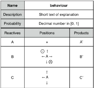
In order to ease the design of behaviours, the authors created a graphical representation consisting of two main parts (see Figure 4). The first part containing three lines indicates the behaviour's name, its description and its probability to occur. The second part is divided in three columns: the left one contains the entities involved in the behaviour (reactive), the middle one indicates where the entities are located one from each other and the right column indicates how entities are changed.

Figure 4. For this example, the behaviour is read like this: “the entity A, which is the centre of the behaviour (+) must be in contact with one entity B and one entity C. B can be anywhere (up, down, left, right, front, behind) around A and C can be at the left, the front or behind A. Moreover, if the probability is validated and the possible conflicts resolved, A will become A', B will become B' and C will be changed in C' ”. The first reactive is always at the centre of the reaction. A reactive or a product can be 0 which means no entity. The diagonals are not taken into account in the positions

In the software NetBioDyn, the graphical user interface is very close in terms of displayed data. The entities are selected thanks to a combo-box containing all the created entities. The positions are selected by clicking on the light or dark squares. The cross at the left allows the user to remove a full line of reactive and products (see Figure 5).

The next subsection describes the environment, where entities are placed and behaviours occur.

3.4. Environment

The environment represents a 2D or 3D space where entities evolve and behaviours take place. It is a simple grid where a grid cell contains none or a maximum of one entity. An entity occupies a whole grid cell. It follows Von Neumann neighbourhood: it has four neighbours in 2D and six in 3D. The size of the environment is by default 100 x 100 x 2 but can be changed by the user. The view is only 2D when the user put, move or remove entities but a 3D view can be activated for a better and more intuitive rendering.

From the principles presented, the next section develops three examples that can be realised by pupils or students

Figure 5. The graphical user interface of behaviours in NetBioDyn has the same properties as seen previously. In this example, an entity A is removed from its current position (first line of the lower part), to be placed at a free location (second line). The third line contains the symbol * as reactive (which means anything) and the symbol - as product (which means do nothing). This behaviour applies a random walk to all A entities in the simulation

4. EXAMPLES

The examples detailed in this section can be performed using the software NetBioDyn freely available at http://virtulab.univ-brest.fr.

It can be made by pupils from age 14 to university students. The first example deals with a prey-predator system involving two species of bacteria: Bdellovibrio and Photobacterium leiognathi. The second example models the dioxygen exchanges between water and the blood of zebra fishes. Finally, the third one aims to reproduce and understand the blood coagulation mechanisms.

These examples show to the students how to create a model in four stages: 1. The Real System

o What is the current knowledge?

o What part of the system would I model?

o What are the limits of my study (dimensions, time, energy, etc.)?

o Am I able to distinguish, among the current knowledge, what are hypothesis and what are facts?

2. The Simplifications

o What have I to keep absolutely from the real system? o What can be neglected?

3. The Model

o How to represent real entities using virtual ones?

o How to model biological mechanisms thanks to algorithms or equations?

o What are the dimensions and the topology of the environment and how to represent it on a computer?

4. The Simulation

o Can I trust the results?

o What are the limits concerning explanation and prediction? o Are the results qualitative or quantitative?

o Does the simulation inspire me in order to prepare real experiments?

o Is the simulation robust to small changes (probabilities or initial state for example)? o Is the simulation clear enough to share and confront my knowledge with others? The next sub-section expose in details the process of modelling three cellular and molecular systems, following these four stages from the real system to the simulation.

4.1. Bdellovibrio and Photobacterium Leiognathi Real System

Bdellovibrio and Photobacterium leiognathi are marine bacteria. The interactions between these two bacteria represent a good example of a predator-prey system. Bdellovibrio is a predator of Photobacterium leiognathi. It penetrates inside its prey, proliferates, kills the host and finally releases its progeny. This cycle time is about 4 hours. Bdellovibrio is a bacterium of 1 µm in size and thanks to its flagellum, moves very fast (up to 160 µm/s). The size of Photobacterium leiognathi is about 2 µm. They usually are in symbiosis with fishes and, in this case, have not shown to be motile.

Biological systems involve too many parameters, objects and behaviours to be fully modelled and simulated. A simplification of the system described here is needed in order to focus on the predator-prey principles.

Simplification

In order to reproduce the Bdellovibrio and Photobacterium leiognathi relationship, a simplified model which takes into account five objects and five behaviours is proposed:  Biological entities:

o Bdellovibrio (Bdel).

o Photobacterium leiognathi (Leio).

o Photobacterium leiognathi infected (LeioInfected).

o Fish tissue where Photobacterium leiognathi lives (FishT).

o Nutriment for Photobacterium leiognathi coming from the fish (Nutri).  Biological behaviours:

o Bdellovibrio movement (BdelMvt).

o Infection of Photobacterium leiognathi by Bdellovibrio (LeioInfection). o Photobacterium leiognathi lyse and Bdellovibrio release (LeioLyse). o Photobacterium leiognathi division (LeioDiv).

o Nutriment production for Photobacterium leiognathi (NutriProd).

This model has to be also adapted to our simulator. The next section explains how to put the model in the software NetBioDyn, which has its own possibilities (i.e. multiple entities and behaviours) and constraints (i.e. the environment is a 3D grid and a grid element has a maximum of six neighbours).

Model

The entities chosen for the simulation are Bdel, Leio and LeioInfected. The fish tissue and the nutriments are implicit in our simulation. This is a choice which can be changed if the fish tissue or the nutriments must be quantitatively taken into account or if their spatial distribution has to be studied. The graphical representation used for entities are simple coloured cubes of volume 1 µm3. In this example Bdel is red, Leio is blue and LeioInfected is purple. Bdel and Leio have a half-life of 100 simulation steps (which means that after 100 simulation steps a Bdel or a Leio entity has 50% of chance to die, or said differently, after 100 simulation steps for a non-reproductive population of N individuals, only N/2 individuals will remain).

Four behaviours have been kept to simulate the bacterial system (see Figure 6):

1. The movement of Bdel entities which is a simple 3D random walk. The probability of this

behaviour is 1.0, the maximum possible, because no other behaviour is as fast as this one. The bibliography gives the speed of 160 µm/s for Bdellovibrio. This is a maximum and an instantaneous speed. Due to its frequent directional changes, its average speed is closer to few µm/s. A grid cell can contain one bacterial entity at the same time, so a grid cell represents a cube of 1 x 1 x 1 µm3.

2. The infection of Leio by Bdel. The probability of infection is 0.1, indicating that one

contact over ten can produce an infection.

3. The lysis of Leio and the release of two Bdel. The probability is chosen to reproduce the 4

hours of incubation for Bdel. A time step is equivalent to one second, so 4 hours are simulated by 14400 steps. At this time, this is supposed that 99% of the LeioInfected have been killed.

4. The division of Leio following the nutriment intake.

The environment is a 100 x 100 x 2 grid. All the Leio entities are at z=0 in order to imitate the fact that they are on the fish tissue.

Simulation and Results

The initial state of the simulation is given by Figure 7. The initial state is made of 1000 Leio entities and 100 Bdel entities randomly located in the environment. Leio entities have been placed at z=0 while Bdel entities are located at z=1. The number of preys is ten times inferior to the number of predators in order to initiate the system without having the preys eaten by too numerous predators at the beginning. They all are located at random in the same 3D environment.

Figure 7. This screen capture of NetBioDyn shows the initial state of the simulation where 1000 Leio (triangles) and 100 Bdel (squares) have been placed at random in the environment using the random initializer tool. Only entities placed at z=0 are here visible

Figure 8 shows two snapshots of the simulation at time steps 1490 and 12840. At time step 1490 (upper screen capture), the first predator-prey cycle is shown, where the Leio population (preys) grows initially, just followed by the growth of the Bdel population (predators). Then, the Leio population decreases because they are eaten by the Bdel, and then the Bdel population decreases too by lack of food, resulting in an increase of Leio due to the fact there are less Bdel entities. The two peaks of the curves are shifted in time: the peak of the preys (Leio) occurs before the peak of predators (Bdel) because the predators need the preys to grow. Small spots of Leio entities appear because of their bacterial division. Five other cycles are shown at the lower part of the figure (time step 12840). The stochastic aspect of the simulation is well shown in the irregularities of curves and entity positions. The predators are close to the preys not because they are attracted by them but simply because they divide inside them. Smaller cycles inside the main cycles can also be seen. Those emerging global behaviours can also be observed in real predator-prey systems (see the Canadian lynx and snowshoe hare pelt-trading records of the Hudson Bay Company over almost a century (Odum, 1953)).

The simulation expresses classical cycles of predator-prey systems, indicating that the results are qualitatively correct.

Figure 8. Screen captures of the simulation at time steps 1490 and 12840. From left to right: the environment states, the population curves of entities Bdel (dark grey) and Leio (light grey) according to time, and the population curve of Leio according to Bdel (after change of the abscissa)

4.2. Water-Blood Dioxygen Exchanges in Zebra Fish Real System

Zebra fishes have an efficient respiratory organ able to extract dioxygen from the water to their blood. Their gills use a counter-current system to improve the dioxygen exchange. Figure 9 represents how the system works. The water contains dioxygen molecules which circulate from the left to the right. A permeable membrane, that only gazes can cross (dotted line), separates the blood from the water. The dioxygen can cross the membrane from the water to the blood or from the blood to the water with exactly the same probability. In the real system, the blood circulates in the opposite direction. However, by using the simulation, the benefits of such mechanism will be studied as compared with the co-current one. The simulation will aim to evaluate the impact of the current direction (counter-current co-current) on the blood oxygenation.

Figure 9. Mechanisms of dioxygen exchange inside the zebra fish gills

Simplification

The simulation focuses on a small part of the system of the Zebra Fish, where the dioxygen exchanges occur. The red blood cells responsible for the transport of the dioxygen in the blood are not modelled, because this mechanism occurs essentially after the exchange. Other blood components, like immune cells for example, are not modelled because they do not interfere in the dioxygen exchange.

Model

The model is made to test the efficiency of the zebra fish counter-current respiratory system where the O2 is central. The chosen model has three types of biological entities, the O2 in various states, and two membranes:

1. The O2 is divided into three types of entity in order to give them different behaviours and count them according to their locations:

o The O2 in water (O2Water). o The O2 in blood (O2Blood).

o The O2 in water which can no longer go to the blood (O2WaterLost) because it has been evacuated outside the respiratory system.

2. The permeable membrane that can be crossed by the O2 (Membrane). 3. The impermeable membrane (Wall).

To complete the model, four dedicated types of entity have been used:

1. Entities O2WaterIn, which perform the addition of O2Water thanks to the behaviour called O2WaterGetIn.

2. Entities O2WaterOut, which remove O2Water thanks to the behaviour O2WaterGetOut. 3. Entities O2BloodOut, which remove O2Blood thanks to the behaviour O2BloodGetOut. 4. Entities O2WaterLostBorder, which detect O2Water entities that can no more go into the

blood thanks to the behaviour O2WaterIsLost.

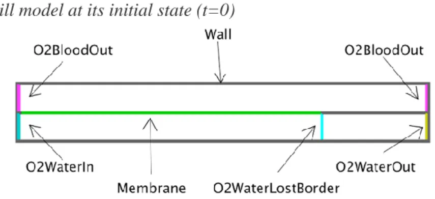
Figure 10 shows how entities are located in their grid environment at t=0.

Figure 10. The gill model at its initial state (t=0)

Only two biological entities are placed: the impermeable membrane (Wall) and the permeable membrane (Membrane) which creates the upper row of blood circulation and the lower row of

water circulation. There is also the four ad-hoc entities (non-biological entities). Note that the O2 is not present at t=0 but will be added at the right to the ad-hoc entities O2WaterIn. When O2 entities in the water diffuse to the right, they can cross the Membrane to go in the blood. The O2 in the blood can also go back to the water by crossing again the Membrane. The O2 entities in water reaching the O2WaterLostBorder can no longer cross the Membrane, and they become lost for the blood (O2WaterLost). The region between O2WaterLostBorder and O2WaterOut only contains O2WaterLost entities that will be counted to test the efficiency of the current and counter-current mechanisms. The O2BloodOut are located at both left and right sides of the upper row in order to evacuate the O2 in the blood whatever the direction the current follows.

Nine behaviours have been made to add movement, membrane crossing, transformation, creation and removal of entities. O2 entities move up, down or right at random in water at each simulation step (probability set to 1). The same mechanism is used to define the movements of O2 in blood and O2WaterLost entities. Note that this behaviour can be modified by changing the left direction by the right, giving the possibility to test the impact of the O2 transfer efficiency from the water to the blood according to the relative direction of both flows.

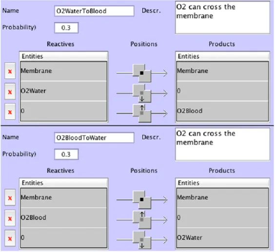
Figure 11 shows how the O2 crosses the membrane. The behaviour indicating how the O2entities in water become lost for the blood is described in Figure 12.

Figure 11. The two behaviours of this figure indicate how O2 entities cross the membrane

separating the blood and the water. The left one concerns the crossing of O2 in water

(O2Water) to the blood (O2Blood). The right one describes the crossing of O2 located in

Finally, Figure 13 shows the only one behaviour that adds entities in the environment. It creates O2Water entities just on the right of O2WaterIn entities with a probability of 0.1. It means that one time step over 10 (on average), one O2WaterIn adds one O2Water (if there is an empty space at its right). The same mechanisms are used to define two more behaviours: the behaviour removing the O2 entities in the water that are too far from the membrane to be useful for the blood (O2WaterLost), and the behaviour removing the O2 entities in blood (probabilities at 1). Defining these behaviours led to create dedicated entities O2WaterIn, O2WaterOut and O2BloodOut that do not exist in the real system. They only are here to simulate the continuous flow of O2 in the water coming from the left and disappearing on the right, when they go out of the simulation area.

Figure 12. This behaviour changes O2Water entities touching the O2WaterLostBorder into O2WaterLost entities. Thus, O2 that cannot be used by the blood can be counted to evaluate

the efficiency of the counter-current mechanism as compared with the current one. The less O2WaterLost entities are present, the more the gills are efficient

Simulation and Results

The simulation using the counter-current behaviour is shown as an example of the dynamics of the gills (see figure 14).

The counting of O2WaterLost gives the efficiency of the system and shows that, for the given initial state and the given behaviours’ parameters, the co-current mechanism is about 42% worse in O2WaterLost as compared with the counter-current one. To evaluate the benefit of the counter-current direction as compared with the same current direction, the number of O2WaterLost has to be counted when the simulation is in a relative permanent state. To calculate when the permanent state arises, we need to know how long it takes for the O2 newly created in water to cross the entire lower compartment. By looking at the behaviour of O2Water (normal or lost), it is clear that the right movement occurs, in average, one time over three (the two other possible movements are up and down). The length of the compartment is about 100. So, at least, 300 time steps are needed for the O2 in the water to run through the lower compartment. Moreover, the O2 can cross the membrane and go back to the left, following the blood flow. About 3/4 of the compartment have the permeable membrane, slowing down the movement of the O2 in the water. Because this is a stochastic simulation, only probabilities can be calculated. The chosen criterion is arbitrary set by looking at the curves of O2LostWater concentration and by choosing a time from which the state looks permanent enough. The average number of O2LostWater is calculated between 1000 and 4000, which seem consistent (see Figure 15).

Figure 14. Three screen captures show how the system evolves when the currents are in opposition (water comes from the left and circulates to the right; blood circulates from the right to the left). At t=150, the O2Water created by the O2WaterGetIn behaviour starts to diffuse to the right of the water compartment (the lower one). The O2Blood entities that reach the O2BloodOut are removed from the simulation thanks to the O2BloodGetOut behaviour. Few O2Blood, coming from the O2Water having crossed the membrane, move in the opposite direction. At t=350, O2Water entities reach the O2WaterLostBorder. At t=2000, the system is in a relatively stable state and O2WaterLost entities can be seen

Figure 15. The average number of O2WaterLost under the co-current condition is 63.4 and 36.7 under the counter-current condition. That makes a loss of O2 which is 42% superior in

the case of co-current. Note that this percentage depends on the size of the compartments and the size of the membrane: this can be easily seen on the screen captures where the density of O2 in water decreases according to the distance from the O2 creation, at the left

4.3. Blood Coagulation Real System

The real system simulated in this example is a small section of a vein, in which a lesion is present. The aim of this model is to reproduce some of the molecular and cellular mechanisms during the blood coagulation leading to the formation of a blood clot. Three stages are usually described. The primary hemostasis starts with the vein lesion and finishes with the formation of a plug covering the lesion. The plug is made of platelets and soluble rod-like shaped proteins called fibrinogen. The secondary hemostasis is the transformation of the platelets plug into a blood clot thanks to the conversion of the fibrinogen into insoluble strands called fibrins. The third and final stage is the fibrinolysis, when the clot is broken down.

Model

The model presented here includes the primary hemostasis but not the secondary one nor the fibrinolysis. Moreover, not all the known mechanisms are simulated to improve the model clarity. The model is described using all the involved entities (cells, molecules and others), their initial state (stored into a 2D matrix) and their behaviours (interactions, transformations, creations and blood flow).

Two types of entities can be distinguished. The first ones are those which directly represent real biological entities like molecules or cells:

1. Fibro (for the fibroblast cells). 2. Endo (for the endothelial cells). 3. PlaC (for the circulating platelets). 4. PlaF (for the fixated platelets). 5. Fibri (for the fibrinogen molecule).

The second ones are those which do not exist as such, but are needed to simulate abstract biological mechanisms, like the blood flow in this case:

1. FlowS (for start of the blood flow). 2. FlowE (for end of the blood flow).

The initial state looks like a rectangle in which the upper edge consists of one layer of endothelial cells. The lower edge contains one layer of endothelial cells (with a discontinuity representing the lesion in the vein) plus one layer of fibroblast cells, below the endothelial layer. The left edge is made of entities regulating the blood flow entrance and the right side consists of entities regulating the blood flow exit (see Figure 16).

The behaviours developed in this simulation aim to model the blood flow and the core mechanisms of primary hemostasis. Firstly, five behaviours are needed to model the blood flow (see Figure 17) :

 One behaviour to model the apparition of the platelets coming from the left of the vein section.

 Two behaviours to model the blood flow circulating from the left to the right which are applied to the platelets (PlaC entities) and the fibrinogens (Fibri entities).

 Two behaviours to model the disappearance of the circulating entities (PlaC and Fibri) when they reach the right of the vein section.

Secondly, three behaviours are needed to model the coagulation (see Figure 18):

 The first behaviour models the fixation of circulating platelets on the lesion (on the fibroblasts).

 The second one models the fixation of circulating platelets on the plug of platelets in presence of fibrinogens.

 The third behaviour models the indirect production of fibrinogens by fibroblasts. Note that this last behaviour is a simplification of a more complex molecular pathway.

The end of the growth of the platelet plug is not modeled thanks to a behaviour but emerges from the simulation. More precisely, when all the fibroblast cells are covered with the anchored platelets, they simply cannot produce fibrinogen, stopping the growth of the plug.

Figure 16. The initial state, and more generally all the simulation, takes place into a 100x28 matrix where entities are distributed according to a simple rectangle corresponding to a vein section. The vein is made-up of three layers, two of endothelial cells (Endo entities) and one layer of fibroblast cells (Fibro entities). Note that the bottom layer of endothelial cells has a hole in order to simulate a lesion, resulting in a direct contact between the fibroblast cells and the circulating blood. The two vertical edges do not exist as real biological entities but are necessary to represent, at the left side of the vein, the incoming of circulating entities (FlowS entities) like the platelets and, at the right side of the vein, the disappearing entities (FlowE entities). The flow of circulating entities moves from the left (Start) to the right (End)

Figure 17. The blood flow is simulated thanks to five behaviours. The two firsts (upper-left) are the movements of circulating platelets and fibrinogens entities from the left to the right. Note that they can also move vertically to reproduce the non-linearity of the blood flow. The third behaviour (upper-right) is the addition of platelets from FlowS (start of flow at the left of the vein section). The probability is 1% and can be changed to simulate different concentrations of platelets (according to the patient for example). The fourth and fifth ones (bottom of the figure) simply remove circulating entities that reach the end of the simulated vein section

Simulation and Results

In the simulation, 1 step corresponds to 1 second. The size of the vein is about 3 millimeter long and 1 millimeter large. As outputs, the shape of the plug is observed and the quantity of circulating fibrinogen is measured at each time step (see Figure 19).

The simulation shows that the plug of platelets starts after 139 steps (2 minutes and 19 seconds) and ends at step 254 (4 minutes and 14 seconds). After this step, no more fibrinogen entity is produced because the fibroblasts are no more in contact with the blood flow. The remaining fibrinogen disappears at the right of the vein section. The simulation is stopped at 360 steps, when all fibrinogen entities have disappeared.

With such a model, it could be possible to use the results of different simulations to build a synthetic and formalised mathematical model of the primary hemostasis. The virtual experiments can be performed quickly and at a very little price. Another interesting feature of such a model is that during a simulation it is possible to create new lesions, change the size or the shape of lesions, modify the platelet concentration, etc. The user can experiment many different scenario and hypothesis and see the validity but also the limits of the model.

Figure 18. The core mechanism governing the apparition of a plug of platelets is only made with three behaviours. The first behaviour (upper-left) is the creation of fibrinogen entities from fibroblast ones. In the real system, it does not occur like this, but it is a convenient simplification for this simple example. The second one is the fixation of circulating platelets that enter in contact with the fibroblast cells of the lesion. The third one, involving three reactive entities, simulates the fixation of circulating platelets onto the plug of anchored platelets, allowing it to grow

Figure 19. After 360 steps of simulation, corresponding to 6 minutes, the plug is formed and the circulating platelets continue to flow from the left to the right (upper diagram of the figure). The quantity of circulating fibrinogen is drawn on the lower part of the figure, showing its growth up to the value of 96 which could be multiplied by a given factor to match real experiments

5. DISCUSSION

Here, the authors discuss the interests and the drawbacks of NetBioDyn. 5.1. NetBioDyn Interests

The use of software in biology and education is interesting, both for teachers and students. It enables teachers to explain complex systems in an intuitive and pseudo-experimental way. It also helps students to create their own computational biological systems and see the important stages by creating a virtual system that rebuilds the real system. They can learn efficiently how the real system works.

From the teacher point of view, the modelling and simulation using such a software enable to:  Create explicative and predictive simulations which can be easily handled by students  Teach the students how to “program” complex systems with very little knowledge in

computer sciences.

 Improve the learning curve of students.  Stimulate students' creativity.

 Quickly find out which students have assimilated the course and which have not.  See where, in the system, a student is right or wrong.

For the students, NetBioDyn gives the possibility to:

 Build or explore biological systems in an intuitive way with entities, behaviours and environments.

 Focus on the main mechanisms of a system and acquire a synthetic view.  Pay attention to important mechanisms even if they look like details.  Learn partially by themselves what is important and what is negligible.  Organise their data and knowledge.

 Play at a motivating construction-like game.

 Explore the impact of parameters or behaviour variations in a simple way.

 Show the teacher what is their comprehension or misunderstanding of the real system.  Share their knowledge with other students in a formal way.

A survey of 30 students (between 22 and 25 years old) has been made to assess the interest of the use of NetBioDyn in class. The results are presented in Figure 20. What is noteworthy is that biologist as well as computer scientist students are mostly interested by such an approach. The question of ease of use for NetBioDyn obtains the most “Very Good” answers for the two master students. Note that this survey is anonymous and that no teacher was present.

This software has also been successfully used by pupils (between 14 and 16 years old) of the middle school Max Jacob in Quimper (France) in May 2011.

5.2. NetBioDyn Drawbacks

The limitations of NetBioDyn can be divided into two kinds. The first concerns the multi-agent approach itself and the second specifically concerns the software.

Multi-agent systems involve many interacting agents. This usually requires powerful computers, in term of computation and memory, to perform all the entities and their interactions. NetBioDyn reduces this problem by only implementing algorithms of complexity N+B (where N is the number of entities and B the number of behaviours). This is possible

because the simulator only uses a small local neighbourhood on a grid. Another problem with multi-agent systems is the number of parameters that can be very important. The simulations made with NetBioDyn could become difficult to control and understand if too many types of entities and behaviours are added. Usually the authors recommend to their students not to add more than 20 types of entity or more than 20 different behaviours. Note that a type of entity is not an entity: a type of entity is a prototype that can be instantiated many times into entities without any problem of parameters.

Regarding the software limitations, the most important one is the entity shape that can only be a cube, implying that the simulations cannot be multi-scale. This last point can be partially circumvented as seen in all the presented examples where molecules, cells and tissues are mingled. For instance, an entity can represent far more than just one molecule, but a group of molecules. An entity can represent a single cell, but also a part of a tissue. What is important here is that an intrinsically multi-scale problem can generally be flattened.

Figure 20. Survey of 24 students in Master 1 Biology and 6 students in Master 2 Computer Science at the Université de Bretagne Occidentale. 10 questions have to be answered on the course they had on computational biology and on the use of the software NetBioDyn. Answers show that both the course and the software are considered important for their training. Moreover, the software is adapted to their skills (no code is required). Finally, the course on modelling and the software interest them and are useful for their studies

6. CONCLUSION

The simulation of complex multi-cellular systems using computers represents a great challenge, both scientifically and technically. Scientifically, it serves the comprehension of fundamental mechanisms governing cells, from single-cell behaviours to whole systems involving numerous interacting cells.

Technically, the creation of computational models imitating multicellular systems requires advanced computational skills.

This is why the authors have developed and presented in this chapter a software making it accessible for non-computer specialists by simplifying the process of modelling and simulation.

This simulator is made to create and manipulate models whereas most of educational software are already-made models that researchers or students can test by only changing some parameters or initial state (see for example the simulator presented in (Meir, Perry, Stal, Maruca, & Klopfer, 2005)).

Three simulations have been presented to show the diversity of models that can be done and to explain how they can be made.

To support this statement, this software has been evaluated by pupils of middle school and higher education students, especially those in the field of biology.

The interest of this software has been discussed to bring out both positive contributions like focusing in what to model instead of how to model but also negative ones like the absence of multi-scale entities.

The perspectives are multiple and can be divided into two parts. Firstly the software itself can be improved. One of the most important features could be the possibility to factorise similar behaviours into one. This could be performed for the entities by adding generic behaviours like Random Walk. Another one is to increase the number of graphical tools to quickly draw shapes of entities like squares, circles or filler. The authors are also working on a self-adjusting system to find the proper values for all the parameters involved in a simulation (behaviours’ probabilities, entities half-lives etc.), in order to stay close to real results obtained for example in vitro.

Secondly, in terms of communication between NetBioDyn users, the main point to address will be the development of an internet social network where researchers, students and teachers will share their works, models and experiences (a starting professional network can be found

at http://lefil.univ-brest.fr then NetBioDyn group).

REFERENCES

Aldrich, C. (2009). The Complete Guide to Simulations and Serious Games. John Wiley & Sons. Ballet, P., Zemirline, A., & Marcé, L. (2004). The Biodyn language and simulators, application to an immune response and E. coli and phage interaction. In Proceeding of the spring school on Modelling and simulation of biological processes in the context of genomics.

Banitz, T., Gras, A., & Ginovart, M. (2015). Individual-based modeling of soil organic matter in NetLogo: Transparent, user-friendly, and open. Environmental Modelling & Software, 71, 39–45. doi:10.1016/j.envsoft.2015.05.007

Bollen, L., & van Joolingen, W.R. (2013). Simsketch: Multiagent simulations based on learner-created sketches for early science education. IEEE Transactions on Learning Technologies, 6(3), 208–216. doi:10.1109/TLT.2013.9

Cock, P.J.A., Antao, T., Chang, J.T., Chapman, B.A., Cox, C.J., Dalke, A., & de Hoon, M.J.L. (2009). Biopython: Freely available Python tools for computational molecular biology and bioinformatics. Bioinformatics (Oxford, England), 25(11), 1422-1423. PMID:19304878.

Epstein, J.M. (1999). Agent-based computational models and generative social science. Complexity, 4(5), 41–60.

doi:10.1002/(SICI)1099-0526(199905/06)4:5<41::AID-CPLX9>3.0.CO;2-F

Gammack, D. (2015). Using NetLogo as a tool to encourage scientific thinking across disciplines. Journal of Teaching and Learning with Technology, 4(1), 22–39. doi:10.14434/jotlt.v4n1.12946 Ginovart, M. (2014). Discovering the power of individual-based modelling in teaching and learning: The study of a predator-prey system. Journal of Science Education and Technology, 23(4), 496–513. doi:10.1007/s10956-013-9480-6

Gkiolmas, A., Karamanos, K., Chalkidis, A., Skordoulis, C., & Papaconstantinou, M.D.S. (2013). Using simulation of Netlogo as a tool for introducing Greek high-school students to eco-systemic thinking. Advances in Systems Science and Application, 13(3), 275–297.

Houser, N. (1992). The Essential Peirce: Selected Philosophical Writings (1867-1893) (Vol. 1). Indiana University Press.

Izaguirre, J.A., Chaturvedi, R., Huang, C., Cickovski, T., Coffland, J., Thomas, G., & Glazier J.A. (2004). Compucell, a multi-model framework for simulation of morphogenesis. Bioinformatics (Oxford, England), 20(7), 1129–1137.

doi:10.1093/bioinformatics/bth05014764549

Jacobson, M.J., & Wilensky, U. (2006). Complex systems in education: Scientific and educational importance and implications for the learning science. Journal of the Learning Sciences, 15(1), 11– 34. doi:10.1207/s15327809jls1501_4

Jenkins, S. (2015). Tools for critical thinking in biology. New York, NY: Oxford University Press.

Kang, S., Kahan, S., McDermott, J., Flann, N., & Shmulevich, I. (2014). Biocellion: Accelerating computer simulation of multicellular biological system models. Bioinformatics (Oxford, England), 30(21), 3101–3108. doi:10.1093/bioinformatics/btu49825064572

Kang, S., Kahan, S., & Momeni, B. (2014). Simulating microbial community patterning using biocellion. In Engineering and Analyzing Multicellular Systems (pp. 233-253). Springer. doi:10.1007/978-1-4939-0554-6_16

Klein, J. (2014). Breve [computer software]. Available from http://www.spiderland.org/breve/

Klein, J., & Spector, L. (2009). 3D Multi-Agent Simulations in the Breve Simulation Environment. In Komosinski, M. & Adamatzky, A. (Eds.), Artificial Life Models in Software (pp. 79–106). Springer. doi:10.1007/978-1-84882-285-6_4

Kubera, Y., Mathieu, P., & Picault, S. (2008). Interaction-oriented agent simulations: From theory to implementation. In Proceedings of the 18th European Conference on Artificial Intelligence (pp. 383-387). IOS Press.

Lynch, S.C., Ferguson, J. (2014). Reasoning about complexity - software models as external representations. In Proceedings of the 25th Workshop of The Psychology of Programming Interest Group.

Meir, E., Perry, J., Stal, D., Maruca, S., & Klopfer, E. (2005). How effective are simulated molecular-level experiments for teaching diffusion and osmosis? Cell Biology Education, 4(3), 235–248. doi:10.1187/cbe.04-09-004916220144

Merks, R.M.H., Guravage, M., Inzé, D., & Beemstaer G.T.S. (2001). VirtualLeaf: An open-source framework for cell-based modelling of plant tissue growth and development. Plant Physiology, 155(2), 656–666. doi:10.1104/pp.110.16761921148415