HAL Id: hal-02340255
https://hal.archives-ouvertes.fr/hal-02340255
Submitted on 30 Oct 2019
HAL is a multi-disciplinary open access
archive for the deposit and dissemination of
sci-entific research documents, whether they are
pub-lished or not. The documents may come from
teaching and research institutions in France or
abroad, or from public or private research centers.
L’archive ouverte pluridisciplinaire HAL, est
destinée au dépôt et à la diffusion de documents
scientifiques de niveau recherche, publiés ou non,
émanant des établissements d’enseignement et de
recherche français ou étrangers, des laboratoires
publics ou privés.
Dynamic load balancing with tokens
Céline Comte
To cite this version:
Céline Comte. Dynamic load balancing with tokens. Computer Communications, Elsevier, 2019, 144,
pp.76-88. �10.1016/j.comcom.2019.05.007�. �hal-02340255�
Dynamic Load Balancing with Tokens
∗
C´
eline Comte
Nokia Bell Labs and T´
el´
ecom ParisTech, University Paris-Saclay, France
[email protected]
October 30, 2019
Abstract
Efficiently exploiting the resources of data centers is a complex task that requires efficient and reliable load balancing and resource allocation algorithms. The former are in charge of assigning jobs to servers upon their arrival in the system, while the latter are responsible for sharing the server resources between their assigned jobs. These algorithms should adapt to various constraints, such as data locality, that restrict the feasible job assignments. In this paper, we propose a token-based algorithm that efficiently balances the load between the servers without requiring any knowledge on the job arrival rates and the server capacities. Assuming a balanced fair sharing of the server resources, we show that the resulting dynamic load balancing is insensitive to the job size distribution. Its performance is compared to that obtained under the best static load balancing and in an ideal system that would constantly optimize the resource utilization. We also make the connection with other token-based algorithms such as Join-Idle-Queue.
Keywords: Load balancing, insensitivity, Whittle networks, order-independent queues.
1
Introduction
The success of cloud services encourages operators to scale out their data centers and optimize the resource utilization. The current trend consists in virtualizing applications instead of running them on dedicated physical resources [1]. Each server may then process several applications at the same time and each appli-cation may be distributed among several servers. Better understanding the dynamics of such server pools is a prerequisite for developing resource management policies that fully exploit this new degree of flexibility.
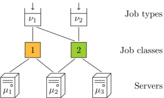
Some recent works have tackled this problem from the point of view of queueing theory [2, 3, 4, 5, 6, 7]. Their common feature is the adoption of a bipartite graph that translates practical constraints, such as data locality, into compatibility relations between jobs and servers. These models can be applied in various systems such as computer clusters, where the shared resource is the CPU [6, 7], and content delivery networks, where the shared resource is the server upload bandwidth [5]. However, these models do not consider the impact of complex load balancing and resource allocation policies simultaneously. The models of [2, 3, 4] lay emphasis on dynamic load balancing, assuming neither server multitasking nor job parallelism. The bipartite graph describes the initial compatibilities of incoming jobs, each of them being eventually assigned to a single server. On the other hand, [5, 6, 7] focus on resource allocation, assuming a static load balancing that assigns incoming jobs to classes at random, independently of the system state. The class of a job in the system subsequently identifies the set of servers that can be pooled to process this job in parallel. The corresponding bipartite graph, connecting classes to servers, restricts the set of feasible resource allocations. In this paper, we introduce a tripartite graph that explicitly differentiates the compatibilities of an incoming job from its actual assignment by the load balancer. This new model allows us to study the joint impact of load balancing and resource allocation. A toy example is shown in Figure 1. Each incoming job
µ1 µ2 µ3 1 2 ν1 ν2 Servers Job classes Job types
Figure 1: A compatibility graph between types, classes, and servers. Two consecutive servers can be pooled to process jobs in parallel: there are two classes, one for servers 1 and 2 and another for servers 2 and 3. Type-1 jobs can be assigned to both classes, while type-2 jobs can only be assigned to the latter. This last restriction may result, for instance, from data locality.
has a type that defines its compatibilities; these may reflect its parallelism degree or locality constraints, for instance. Depending on the system state, the load balancer matches the job with a compatible class that subsequently defines its assigned servers. The upper part of our graph, which puts constraints on load balancing, corresponds to the bipartite graph of [2, 3, 4]; the lower part, which restricts the resource allocation, corresponds to the bipartite graph of [5, 6, 7].
We use this new framework to study resource management policies that are insensitive, in the sense that they make the system performance independent of fine-grained traffic characteristics. This property is highly desirable, as it allows service providers to dimension their infrastructure based on average traffic predictions only. It has been extensively studied in the queueing literature [5, 8, 9, 10]. In particular, insensitive load balancing policies were introduced in [10] in a generic queueing model, assuming an arbitrary insensitive allocation of the resources. These insensitive load balancing policies were defined as a generalization of the static policy described above, in which the assignment probabilities of jobs to classes depend on the system state and are chosen to preserve the insensitivity of the resource allocation.
Our main contribution is an algorithm based on tokens that enforces such an insensitive load balancing without performing randomized assignments. This deterministic algorithm can operate under any compati-bility graph, without requiring any knowledge of the job arrival rates and server capacities. Each assignment decision is based solely on the compatibilities of the incoming job and the current system state. The principle is as follows. The load balancer keeps a queue that is initially filled with a fixed number of available tokens of each class. An incoming job seizes the longest available token among those that identify a compatible class, and is blocked if it does not find any. The rationale behind this algorithm is to use the release order of tokens as an information on the relative load of their servers: a token that has been available for a long time without being seized is likely to identify a server set that is less loaded than others. As we will see, our algorithm mirrors the first-come, first-served (FCFS) service discipline proposed in [7] to implement balanced fairness, which was defined in [9] as the most efficient insensitive resource allocation. It also extends the algorithm which was initially proposed in [3] for server pools without server multitasking nor job parallelism.
Organization of the paper Section 2 recalls known results on resource allocation in server pools. We describe a standard server pool model based on a bipartite compatibility graph and explain how balanced fairness is applied in this model. Section 3 contains our main contributions. We propose a model based on a tripartite graph and introduce a new token-based insensitive load balancing algorithm. The numerical results are presented in Section 4 and the related works in Section 5. Section 6 concludes the paper.
2
Resource allocation
We first recall the model considered in [5, 6, 7] to study the problem of resource allocation in server pools. This model will be extended in Section 3 to integrate dynamic load balancing.
2.1
Model
We consider a pool of S servers. There are N job classes and we let I = {1, . . . , N } denote the set of class indices. For now, each incoming job is assigned to a compatible class at random, independently of the system state. For each i ∈ I, the resulting arrival process of jobs assigned to class i is assumed to be Poisson with a rate λi > 0 that may depend on the job arrival rates, compatibilities and assignment probabilities. We also
assume that the number of jobs of class i in the system is limited by ℓi, for each i ∈ I, so that a new job
is blocked if its assigned class is already full. Job sizes are independent and exponentially distributed with unit mean. Each job leaves the system immediately after service completion.
The class of a job defines the set of servers that can be pooled to process it. Specifically, for each i ∈ I, a job of class i can be served in parallel by any subset of servers within the non-empty set Si⊂ {1, . . . , S}.
This defines a bipartite compatibility graph between classes and servers, where there is an edge between a class and a server if the jobs of this class can be processed by this server. Figure 2 shows a toy example.
µ1 µ2 µ3
λ1 λ2
Servers Job classes
Figure 2: A compatibility graph between classes and servers. Servers 1 and 3 are dedicated, while server 2 can serve both classes. The server sets associated with classes 1 and 2 are S1 = {1, 2} and S2 = {2, 3},
respectively.
When a job is in service on several servers, its service rate is the sum of the rates allocated by each server to this job. For each s = 1, . . . , S, the capacity of server s is denoted by µs > 0. We can then define a
function µ on the power set of I as follows: for each A ⊂ I,
µ(A) = X
s∈Si∈ASi
µs
denotes the aggregate capacity of the servers that can process at least one class in A, i.e., the maximum rate at which jobs of these classes can be served. As observed in [5], the function µ is a rank function because it satisfies the following properties:
Normalization µ(∅) = 0;
Monotonicity For each class sets A, B ⊂ I such that A ⊂ B, we have µ(A) ≤ µ(B);
Submodularity For each class sets A, B ⊂ I such that A ⊂ B and each class i /∈ B, we have: µ(A ∪ {i}) − µ(A) ≥ µ(B ∪ {i}) − µ(B).
2.2
Balanced fairness
We recall the definition of balanced fairness [9] which was first applied to server pools in [5]. Like processor sharing (PS) policy, balanced fairness assumes that the capacity of each server can be divided continuously between its jobs. It is further assumed that the resource allocation only depends on the number of jobs of each class in the system; in particular, all jobs of the same class receive service at the same rate.
The system state is given by the vector x = (xi: i ∈ I) of the numbers of jobs of each class in the system.
The state space is X = {x ∈NN : x ≤ ℓ}, whereN is the set of non-negative integers, ℓ = (ℓ
vector of per-class constraints, and the comparison ≤ is taken componentwise. For each i ∈ I, we let φi(x)
denote the total service rate allocated to class-i jobs in state x. It is assumed to be nonzero if and only if xi > 0, in which case each job of class i receives service at rate φix(x)i .
Queueing model Since all jobs of the same class receive service at the same rate, we can describe the evolution of the system with a network of N PS queues with state-dependent service capacities. For each i ∈ I, queue i contains the jobs of class i; the arrival rate at this queue is λiand its service capacity is φi(x)
when the network state is x. An example is shown in Figure 3 for the configuration of Figure 2.
φ1(x) x1= 3 λ1 φ2(x) x2= 2 λ2
Figure 3: An open Whittle network of N = 2 queues associated with the pool of Figure 2. As in Figures 4, 5, 7, and 8, we assume at most ℓ1= ℓ2= 4 jobs can be assigned to each class.
Capacity set The compatibilities between classes and servers restrict the set of feasible resource alloca-tions. Specifically, the vector (φi(x) : i ∈ I) of per-class service rates belongs to the following capacity set
in any state x ∈ X : Σ = ( φ ∈RN + : X i∈A φi≤ µ(A), ∀A ⊂ I ) . Since µ is a rank function, the set Σ is a polymatroid [11].
Balance function It was shown in [8] that the resource allocation is insensitive if and only if there is a balance function Φ defined on X such that Φ(0) = 1 and
φi(x) = Φ(x − ei)
Φ(x) , ∀x ∈ X , ∀i ∈ I(x), (1)
where ei∈NN is the unit vector with 1 in component i and 0 elsewhere, and I(x) = {i ∈ I : xi> 0} is the
set of active classes in state x. Under this condition, the network of PS queues defined above is a Whittle network [12]. The insensitive resource allocations that respect the capacity constraints of the system are characterized by a balance function Φ such that, for all x ∈ X \ {0},
Φ(x) ≥ 1
µ(A) X
i∈A
Φ(x − ei), ∀A ⊂ I(x) : A 6= ∅.
Recursively maximizing the overall service rate in the system is then equivalent to minimizing Φ by choosing Φ(x) = max A⊂I(x): A6=∅ 1 µ(A) X i∈A Φ(x − ei) ! , ∀x ∈ X \ {0}.
The resource allocation defined by this balance function is called balanced fairness.
It was shown in [5] that balanced fairness is Pareto-efficient in polymatroid capacity sets, meaning that the total service rateP
i∈I(x)φi(x) is always equal to the aggregate capacity µ(I(x)) of the servers that can
process at least one active class. By (1), this means that the maximum in the recursive definition of Φ is always attained at the set of active classes, that is,
Φ(x) = 1
µ(I(x)) X
i∈I(x)
Stationary distribution The Markov process defined by the system state x is reversible, with stationary distribution
π(x) = π(0)Φ(x)Y
i∈I
λixi, ∀x ∈ X . (3)
By insensitivity, the system state has the same stationary distribution if the jobs sizes within each class are only i.i.d., as long as the traffic intensity of class i (defined as the average quantity of work brought by jobs of this class per unit of time) is λi, for each i ∈ I. A proof of this result is given in [8] for Cox distributions,
which form a dense subset within the set of distributions of non-negative random variables.
2.3
Job scheduling
We now describe the sequential implementation of balanced fairness that was proposed in [7]. This will lay the foundations for the results of Section 3.
Algorithm We still assume that jobs can be distributed among several servers, but we relax the assumption that servers can process several jobs at the same time. Instead, each server processes its jobs sequentially in FCFS order. When a job arrives, it enters in service on every idle server within its assignment, if any, so that its service rate is the sum of the capacities of these servers. When the service of a job is complete, this job leaves the system immediately and its servers are reallocated to the first job they can serve in the queue. Note that this sequential implementation also makes sense in a model where jobs are replicated instead of being processed in parallel. For more details, the reader can refer to [6] where the model with redundant requests was introduced.
Since the arrival order of the jobs impacts the rate allocation, we need to detail the system state. We consider the sequence c = (c1, . . . , cn), where n ≤Pi∈Iℓiis the total number of jobs in the system and, for
each p = 1, . . . , n, cp∈ I is the class of the p-th oldest job (in particular, c1corresponds to the job that has
been present the longest). The empty state, with n = 0, is denoted by ∅. To each such detailed state c, we can associate an aggregate state |c| = ec1+ ec2+ . . . + ecn ∈ X that coincides with the state introduced in
§2.2: for each i ∈ I, the integer |c|i counts the number of class-i jobs in the sequence c. This aggregate state
does not define a Markov process in general. The state space of the detailed state is C = {c ∈ I∗: |c| ≤ ℓ}, where I∗ is the Kleene star of I. Note that we will often use the same letter to define functions of the detailed state c and of the corresponding aggregate state |c|. For instance, I(c) = I(|c|) will denote the set of active classes in state c. Since the detailed and aggregate states belong to two disjoint sets, there is no ambiguity.
Queueing model Each job is in service on all the servers that were assigned this job but not those that arrived earlier. For each p = 1, . . . , n, the service rate of the job in position p is thus given by
X
s∈Scp\Sp−1q=1Scq
µs= µ(I(c1, . . . , cp)) − µ(I(c1, . . . , cp−1)),
with the convention that (c1, . . . , cp−1) = ∅ if p = 1. The service rate of a job is independent of the jobs
arrived later in the system. Additionally, the total service rate µ(I(c)) is independent of the arrival order of jobs. The corresponding queueing model is an order-independent (OI) queue [13, 14]. An example is shown in Figure 4 for the configuration of Figure 2.
Stationary distribution The system state c defines an irreducible Markov process. According to [14], this process is quasi-reversible [12, 15], with stationary distribution
π(c) = π(∅)Φ(c)Y
i∈I
2 1 2 1 1 c = (1, 1, 2, 1, 2) µ1 µ2 µ3 λ1 λ2
Figure 4: An OI queue with N = 2 job classes associated with the pool of Figure 2. The colors of the servers indicate the jobs they are processing. The first job of class 1, at the head of the queue, is in service on servers 1 and 2. The first job of class 2, in third position, is in service on server 3. Aggregating the state c yields the state x of the Whittle network of Figure 3.
where Φ is defined recursively on C by Φ(∅) = 1 and
Φ(c) = 1
µ(I(c))Φ(c1, . . . , cn−1), ∀c ∈ C \ {∅}. (5)
We go back to the aggregate state x that gives the number of jobs of each class in the system. It turns out that we have
Φ(x) = X
c:|c|=x
Φ(c) and π(x) = X
c:|c|=x
π(c), ∀x ∈ X ,
where Φ(x) and π(x) are as defined by (2) and (3); in particular, the aggregate state x has the same stationary distribution under the FCFS scheduling as under balanced fairness. The first equality can be shown using (2) and (5). We can then use (3) and (4) to prove the second equality: for each x ∈ X ,
X c:|c|=x π(c) = π(∅) X c:|c|=x Φ(c) Y i∈I λixi = π(0)Φ(x) Y i∈I λixi = π(x).
It was also shown in [7] that the average per-class resource allocation resulting from the FCFS service discipline is balanced fairness. More precisely, we have
φi(x) =
X
c:|c|=x
π(c)
π(x)µi(c), ∀x ∈ X , ∀i ∈ I(x),
where φi(x) is the total service rate allocated to class-i jobs in state x under balanced fairness, given by (1),
and µi(c) is the service rate received by the first job of class i in state c under the FCFS service discipline:
µi(c) = n X p=1 cp=i (µ(I(c1, . . . , cp)) − µ(I(c1, . . . , cp−1))).
We will later use the following equality, which is obtained by injecting (3) and (4) in the rate equality: φi(x) =
X
c:|c|=x
Φ(c)
Φ(x)µi(c), ∀x ∈ X , ∀i ∈ I(x). (6)
As it is, the FCFS service discipline is very sensitive to the job size distribution. [7] mitigates this sensitivity by frequently interrupting jobs and moving them to the end of the queue, in the same way as round-robin scheduling algorithm in the single-server case. The pseudocode of this scheduling algorithm is given in [7]. In the queueing model, the interruptions and resumptions are represented approximately by random routing, which leaves the stationary distribution unchanged by quasi-reversibility [12, 15]. If the interruptions are frequent enough, then all jobs of a class tend to receive the same service rate on average, which is that obtained under balanced fairness. In particular, the performance becomes approximately insensitive to the job size distribution within each class.
3
Load balancing
The previous section has considered the problem of resource sharing. We now focus on dynamic load balancing, using the fact that each job may be a priori compatible with several classes and assigned to one of them upon arrival. We first extend the model of §2.1 to add this new degree of flexibility.
3.1
Model
We again consider a pool of S servers. There are N job classes and we let I = {1, . . . , N } denote the set of class indices. The compatibilities between job classes and servers are described by a bipartite graph, as explained in §2.1. Additionally, we assume that the arrivals are divided into K types, so that the jobs of each type enter the system according to an independent Poisson process. Job sizes are independent and exponentially distributed with unit mean. Each job leaves the system immediately after service completion. The type of a job defines the set of classes it can be assigned to. This assignment is performed instan-taneously upon the job arrival, according to some decision rule that will be detailed later. For each i ∈ I, we let Ki ⊂ {1, . . . , K} denote the non-empty set of job types that can be assigned to class i. This defines a
bipartite compatibility graph between types and classes, where there is an edge between a type and a class if the jobs of this type can be assigned to this class. Overall, the compatibilities are described by a tripartite graph between types, classes, and servers, as illustrated in Figure 1. Without loss of generality, we can assume that all the classes are separable in the sense that, for each i, j ∈ I with i 6= j, we have Si 6= Sj or
Ki 6= Kj (otherwise, we can aggregate these classes). We will use this assumption to prove the irreducibility
of the Markov process considered in §3.3.
For each k = 1, . . . , K, the arrival rate of type-k jobs in the system is denoted by νk > 0. We can then
define a function ν on the power set of I as follows: for each A ⊂ I,
ν(A) = X
k∈Si∈AKi
νk
denotes the aggregate arrival rate of the types that can be assigned to at least one class in A. This function ν is a rank function, for the same reason as the function µ defined in §2.1.
3.2
Randomized load balancing
We now express the insensitive load balancing of [10] in our new server pool model. This extends the static load balancing considered earlier. Incoming jobs are assigned to classes at random, and the assignment probabilities depend not only on the job type but also on the system state. As in §2.2, we assume that the capacity of each server can be divided continuously between its jobs. The resources are allocated by applying balanced fairness in the capacity set Σ defined by the bipartite compatibility graph between classes and servers.
Open queueing model We first adapt the queueing model considered in [10] to describe the randomized load balancing. As in §2.2, jobs are gathered class-by-class in PS queues with state-dependent service capacities given by (1). In particular, the type of a job is forgotten once it is assigned to a class.
Similarly, we record the job arrivals depending on the class they are assigned to, regardless of their type before the assignment. The Poisson arrival assumption ensures that, given the system state, the time before the next arrival to each class is exponentially distributed and independent of the arrivals at other classes. The rates of these arrivals result from the load balancing. We write them as functions of the vector y = ℓ − x of numbers of available positions at each class. Specifically, λi(y) denotes the arrival rate of jobs assigned to
class i when there are yj available positions in class j, for each j ∈ I.
The system can thus be modeled by a network of N PS queues with state-dependent arrival rates, as shown in Figure 5a.
φ1(x) x1= 3 φ2(x) x2= 2 λ1(ℓ − x) λ2(ℓ − x)
(a) An open Whittle network with state-dependent arrival rates. λ1(y) y1= 1 λ2(y) y2= 2 φ1(x) x1= 3 φ2(x) x2= 2 Class-1 tokens Class-2 tokens
(b) A closed queueing model consisting of two Whittle networks.
Figure 5: Alternative representations of a Whittle network associated with the pool of Figure 1.
Closed queueing model We introduce a second queueing model that describes the system dynamics differently. It will later simplify the study of the insensitive load balancing by drawing a parallel with the resource allocation of §2.2.
Our alternative model stems from the following observation: since we impose limits on the number of jobs of each class, we can indifferently assume that the arrivals are controlled by the intermediary of another set of queues that contain the available tokens. Specifically, for each i ∈ I, the assignments to class i are controlled through a queue that is initially filled with ℓi tokens. A job that is assigned to class i removes a
token from this queue and holds it until its service is complete. The assignments to a class are suspended when its queue of available tokens is empty, and resumed when a token of this class is released.
Each token is either held by a job in service or waiting to be seized by an incoming job. Our alternative closed queueing model reflects this alternation: a first network of N queues contains the tokens held by jobs in service, as before, and a second network of N queues contains the available tokens. For each i ∈ I, a token of class i alternates between the queues indexed by i in the two networks. This is illustrated in Figure 5b.
The state of the network that contains the tokens held by jobs in service is x. The queues in this network apply PS service discipline and their service capacities are given by (1). The state of the network that contains the available tokens is y = ℓ − x. For each i ∈ I, the service of a token at queue i in this network is triggered by the arrival of a job assigned to class i. The service capacity of this queue is thus equal to λi(y)
in state y. Since all tokens of the same class are exchangeable, we can assume indifferently that we pick one of them at random, so that the service discipline is again PS.
Capacity set The compatibilities between the job types and the classes restrict the set of feasible load balancings. Specifically, the vector (λi(y) : i ∈ I) of per-class arrival rates belongs to the following capacity
set in any state y ∈ X :
Γ = ( λ ∈RN + : X i∈A λi ≤ ν(A), ∀A ⊂ I ) . Since ν is a rank function, the set Γ is a polymatroid.
Balance function It was shown in [10] that the load balancing is insensitive if and only if there is a balance function Λ defined on X such that Λ(0) = 1 and
λi(y) =
Λ(y − ei)
Λ(y) , ∀y ∈ X , ∀i ∈ I(y). (7)
Under this condition, the network of PS queues containing the available tokens is a Whittle network. Our token-based reformulation allows us to interpret dynamic load balancing as a problem of resource allocation in this Whittle network, in which we can apply the results §2.2. In particular, the Pareto-efficiency of balanced fairness in polymatroid capacity sets can be understood as follows in terms of the load balancing.
We consider the balance function Λ defined recursively on X by Λ(0) = 1 and Λ(y) = 1 ν(I(y)) X i∈I(y) Λ(y − ei), ∀y ∈ X \ {0}. (8)
Then Λ defines a load balancing that belongs to the capacity set Γ in each state y ∈ X . By (7), this load balancing satisfies
X
i∈I(y)
λi(y) = ν(I(y)), ∀y ∈ X ,
meaning that an incoming job is accepted whenever it is compatible with at least one available token. Stationary distribution The Markov process defined by the system state (x, y) is reversible, with sta-tionary distribution
π(x, y) = 1
GΦ(x)Λ(y), ∀x, y ∈ X : x + y = ℓ, (9)
where G is a normalization constant. Note that we could also focus on either state x or y and retrieve the other with the equality x + y = ℓ. Also, as mentioned earlier, the insensitivity of balanced fairness is preserved by the load balancing.
3.3
Deterministic token mechanism
Our closed queueing model reveals that the randomized load balancing is dual to the balanced fair resource allocation. This allows us to propose a new deterministic load balancing algorithm that mirrors the FCFS service discipline of §2.3. This algorithm can be combined indifferently with balanced fairness or with the FCFS scheduling; in both cases, we show that it implements the load balancing defined by (7).
Algorithm All the available tokens are now sorted in order of release in a single queue. The longest available tokens are in front. An incoming job scans this queue from beginning to end and seizes the first compatible token; it is blocked if it does not find any. For now, we assume that the server resources are allocated to the accepted jobs by applying the FCFS service discipline of §2.3. When the service of a job is complete, its released token is appended to the queue of available tokens.
The detailed system state is now given by the couple (c, d) that retains both the job arrival order and the token release order. Specifically, c = (c1, . . . , cn) ∈ C is the sequence of classes of (tokens held by) jobs in
service, as before, and d = (d1, . . . , dm) ∈ C is the sequence of classes of available tokens, ordered by release.
The aggregate state, which coincides with the state introduced in §3.2, is (x, y) with x = |c| and y = |d|. Given the total number of tokens of each class in the system, any feasible state satisfies |c| + |d| = ℓ.
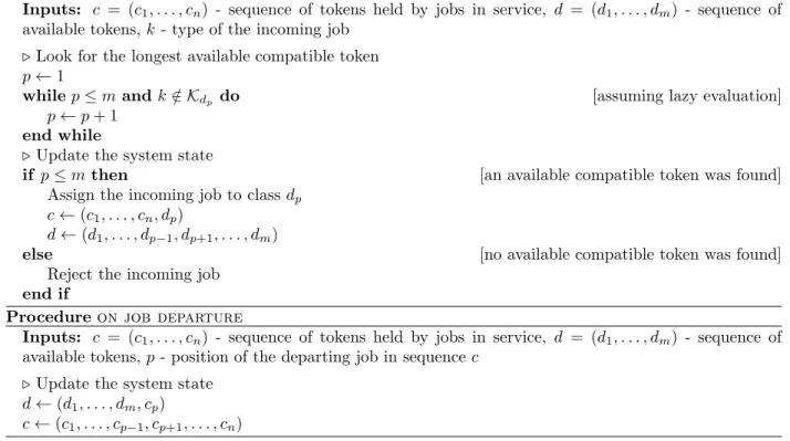
The pseudocode of the algorithm is given in Figure 6. A key performance criterion is the complexity of the assignment decision, defined as the number of operations to perform upon a job arrival. A priori, it can be as high as the length m of the queue of available tokens, which is upper-bounded by the total number P
i∈Iℓiof tokens. To reduce the complexity, we can take the assignment decision based on a second list that
only retains the order of the first available tokens of each class, and update this list after each arrival or departure. Then the complexity is upper-bounded by the number N of classes, and can be further reduced if, for instance, a subset of the classes is known to share the same compatibilities with job types. Alternatively, if the incoming job types are known in advance, the complexity can be made constant by storing the class each job type should be assigned to upon arrival.
Queueing model Depending on its position in the queue, each available token is seized by any incoming job whose type is compatible with this token but not with the tokens released earlier. For each p = 1, . . . , m, the token in position p is thus seized at rate
X
k∈Kdp\Sp−1q=1Kdq
Procedure on job arrival
Inputs: c = (c1, . . . , cn) - sequence of tokens held by jobs in service, d = (d1, . . . , dm) - sequence of
available tokens, k - type of the incoming job ⊲ Look for the longest available compatible token p ← 1
while p ≤ m and k /∈ Kdp do [assuming lazy evaluation]
p ← p + 1 end while
⊲ Update the system state
if p ≤ m then [an available compatible token was found]
Assign the incoming job to class dp
c ← (c1, . . . , cn, dp)
d ← (d1, . . . , dp−1, dp+1, . . . , dm)
else [no available compatible token was found]
Reject the incoming job end if
Procedure on job departure
Inputs: c = (c1, . . . , cn) - sequence of tokens held by jobs in service, d = (d1, . . . , dm) - sequence of
available tokens, p - position of the departing job in sequence c ⊲ Update the system state
d ← (d1, . . . , dm, cp)
c ← (c1, . . . , cp−1, cp+1, . . . , cn)
Figure 6: Token-based load balancing algorithm. Note that the first procedure could also take as an input the set of token classes that are compatible the incoming job instead of its type.
The seizing rate of a token is independent of the tokens released later. Additionally, the total rate at which available tokens are seized is ν(I(d)), independently of their release order. The queue of available tokens can thus be modeled by an OI queue, where the service of a token is triggered by the arrival of a job that seizes this token.
The evolution of the sequence of tokens held by jobs in service also defines an OI queue, with the same dynamics as in §2.3. Overall, the system can be modeled by a closed tandem network of two OI queues, as shown in Figure 7. 2 1 2 1 1 c = (1, 1, 2, 1, 2) µ1 µ2 µ3 1 2 2 d = (1, 2, 2) ν1 ν2
Figure 7: A closed tandem network of two OI queues associated with the pool of Figure 1. The detailed state is (c, d), with c = (1, 1, 2, 1, 2) and d = (1, 2, 2). The corresponding aggregate state is that of the network of Figure 5. An incoming job of type 1 would seize the available token in first position, of class 1, while an incoming job of type 2 would seize the available token in second position, of class 2.
Stationary distribution The Markov process defined by the detailed state (c, d) is irreducible. The proof is given in the appendix. Known results on closed networks of quasi-reversible queues [15, 12] then show
that this process is quasi-reversible, with stationary distribution π(c, d) = 1
GΦ(c)Λ(d), ∀c, d ∈ C : |c| + |d| = ℓ, (10)
where G is a normalization constant, Φ is defined by recursion (5) and the initial step Φ(∅) = 1, as in §2.3, and Λ is defined recursively on C by Λ(∅) = 1 and
Λ(d) = 1
ν(I(d))Λ(d1, . . . , dm−1), ∀d ∈ C \ {∅}. (11)
We go back to the aggregate state (x, y) that counts the number of tokens of each class that are either held by jobs in service or available. Similarly to §2.3, we prove that its stationary distribution is given by (9). We can first use (2), (5), (8), and (11) to show that, for each x, y ∈ X , we have
Φ(x) = X
c:|c|=x
Φ(c) and Λ(y) = X
d:|d|=y
Λ(d). (12)
Then we conclude by applying (9) and (10): for each x, y ∈ X such that x + y = ℓ, we have X c:|c|=x, d:|d|=y π(c, d) = 1 G X c:|c|=x Φ(c) X d:|d|=y Λ(d) = 1 GΦ(x)Λ(y) = π(x, y).
The average per-class service rates are still as defined by balanced fairness. Indeed, we can use (12) to rewrite (6) as follows: for each x ∈ X and i ∈ I(x), we have
φi(x) = X c:|c|=x 1 GΦ(c) P d:|d|=ℓ−xΛ(d) 1 GΦ(x)Λ(ℓ − x) µi(c) = X c:|c|=x X d:|d|=ℓ−x π(c, d) π(x, ℓ − x)µi(c).
By symmetry, it follows that the average per-class arrival rates, ignoring the release order of tokens, are as defined by the randomized load balancing. Specifically, for each y ∈ X and i ∈ I(y), we have
λi(y) = X c:|c|=ℓ−y X d:|d|=y π(c, d) π(ℓ − y, y)νi(d),
where λi(y) is the arrival rate of jobs assigned to class i in state y under the randomized load balancing, given
by (7), and νi(d) is the rate at which the longest available token of class i is seized under the deterministic
load balancing: νi(d) = m X p=1 dp=i (ν(I(d1, . . . , dp)) − ν(I(d1, . . . , dp−1))).
As in §2.3, the stationary distribution of the system state is unchanged by the addition of random routing, as long as the average traffic intensity of each class remains constant. Hence we can again reach some approximate insensitivity to the job size distribution within each class by enforcing frequent job interruptions and resumptions.
Application with balanced fairness As announced earlier, we can also combine our token-based load balancing algorithm with balanced fairness rather than the FCFS scheduling. The assignment of jobs to classes is still regulated by a single queue containing all available tokens, sorted in release order, but the resources are now allocated according to balanced fairness. The corresponding queueing model consists of an OI queue and a Whittle network, as represented in Figure 8.
1 2 2 d = (1, 2, 2) ν1 ν2 φ1(x) x1= 3 φ2(x) x2= 2 Class-1 tokens Class-2 tokens
Figure 8: A closed queueing model, consisting of an OI queue and a Whittle network, associated with the pool of Figure 1.
The intermediary state (x, d), retaining the release order of available tokens but not the arrival order of jobs, defines a Markov process. Its stationary distribution follows from known results on networks of quasi-reversible queues [12, 15]:
π(x, d) = 1
GΦ(x)Λ(d), ∀x ∈ X , ∀d ∈ C : x + |d| = ℓ.
We can show as before that the average per-class arrival rates, ignoring the release order of tokens, are as defined by the dynamic load balancing of §3.2.
The insensitivity of balanced fairness to the job size distribution within each class is again preserved. The proof of [8] for Cox distributions extends directly. Note that this does no imply that performance is insensitive to the job size distribution within each type. Indeed, if two job types with different size distributions can be assigned to the same class, then the distribution of the job sizes within this class may be correlated to the system state upon their arrival. This point will be assessed by simulation in Section 4.
Observe that our token-based mechanism can be applied to balance the load between the queues of an arbitrary Whittle network, as represented in Figure 8, independently of the system considered. Examples or such systems are given in [10].
Application with a static resource allocation Finally, let us briefly detail the special case in which each class gives access to a single dedicated server. The lower part of the tripartite assignment graph is trivial (there is a one-to-one association between classes and servers), while the upper part describes the compatibilities between incoming jobs and servers. In other words, we have S = N and, for each i ∈ I, Si = {i}. Applying balanced fairness is equivalent to applying PS policy at each server, and applying the
FCFS scheduling described in §2.3 is equivalent to individually applying FCFS service discipline at each server. The token-based algorithm assigns incoming jobs to one of their compatible servers depending on their relative loads. This scenario was extensively studied in [2, 3, 4] in the special case in which each server has a single token (see Section 5 for more details).
The queueing model we obtain is symmetrical to that of Section 2. Under the FCFS scheduling, we can divide the queue of tokens held by jobs in service into as many independent queues as there are servers. The detailed state d = (d1, . . . , dm) ∈ C of the queue of available tokens defines a Markov process, with stationary
distribution:
π(d) = π(∅)Λ(d)Y
i∈I
µi|d|i, ∀d ∈ C.
This is the counterpart of (4). Similarly, the stationary distribution of the aggregate state y is the counterpart of (3):
π(y) = π(0)Λ(y)Y
i∈I
4
Numerical results
The objective of this section is both to illustrate how we can apply the formulas of Section 3 and to better understand the impact of the token-based algorithm in simple examples. The code is available on Github [16].
4.1
Compute the performance metrics
We first define some performance metrics and express them in our model. By insensitivity, the obtained formulas also give the performance when the job sizes within each class are i.i.d., as long as the traffic intensity is unchanged.
Occupancy ratios For each k = 1, . . . , K, we let βk=
X
y≤ℓ: k /∈Si∈I(y)Ki
π(ℓ − y, y)
denote the probability that a job of type k is blocked upon arrival. The equality follows from PASTA property [12]. Symmetrically, for each s = 1, . . . , S, we let
ψs=
X
x≤ℓ: s /∈Si∈I(x)Si
π(x, ℓ − x)
denote the probability that server s is idle. These quantities are related by the conservation equation
K X k=1 νk(1 − βk) = S X s=1 µs(1 − ψs). (13)
We define respectively the average blocking probability and the average resource occupancy by β = PK k=1νkβk PK k=1νk and η = PS s=1µs(1 − ψs) PS s=1µs . There is a simple relation between β and η. Indeed, if ρ = (PK
k=1νk)/(PSs=1µs) denotes the total load in
the system, we can rewrite (13) as ρ(1 − β) = η.
As expected, minimizing the average blocking probability is equivalent to maximizing the average resource occupancy. It is convenient, however, to look at both metrics in parallel. As we will see, when the system is underloaded, jobs are almost never blocked and it is easier to describe the (almost linear) evolution of the resource occupancy. On the contrary, when the system is overloaded, resources tend to be maximally occupied and it is more interesting to focus on the blocking probability.
Observe that any stable server pool satisfies the conservation equation (13), irrespective of the resource management policy. In particular, the average blocking probability β in a stable system cannot be less than 1 − 1ρ when ρ > 1. A similar argument applied to each job type individually imposes that
βk ≥ max 0, 1 − 1 νk X s∈Si:k∈KiSi µs , (14) for each k = 1, . . . , K.
Mean number of jobs For each i ∈ I, we let Li= X x∈X xi× π(x, ℓ − x) = ℓi− X y∈X yi× π(ℓ − y, y)
denote the mean number of jobs of class i in the system, that is, the mean number of class-i tokens that are held by jobs in service. By Little’s law [12], the mean delay δi of the jobs assigned to class i is the ratio of
the mean number of jobs of this class in the system to their effective arrival rate: δi= Li P y≤ℓλi(y)π(ℓ − y, y) =P Li x≤ℓφi(x)π(x, ℓ − x) .
The second equality follows by conservation. We also define the mean service rate γi as the mean service
speed perceived by the jobs in service within class i. Taking the mean job size as the unit, it is simply the inverse of the mean delay: γi=δ1
i.
We also let L = P
i∈ILi denote the mean number of jobs in the system, irrespective of their assigned
class. Again, by Little’s law, the mean delay δ is given by
δ = L PK k=1νk(1 − βk) = L PN s=1µs(1 − ψs) ,
where the second equality follows from (13). The mean service rate γ perceived by the jobs in service is given by γ = 1δ.
Let us recall that the system state does not retain the number of jobs of each type that are present. Hence, in general, we cannot use the stationary distribution to compute the mean delay or the mean service rate of each job type. A notable exception is the case where a job type has an exclusive set of compatible classes, that is, it is the only job type that can be assigned to its compatible classes, as shown in Figure 9. Simulation settings We rely on simulations to compute the metrics that cannot be predicted by the model. Each simulation point is the average of 100 independent runs, each built up of 106 jumps after a
warm-up period of 106 jumps. The asymptotic 95% confidence intervals, not shown on the figures, do not
exceed ±0.0001 around the points for the blocking probability and ±0.007 for the mean number of jobs.
4.2
A single job type
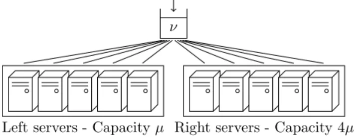
We first consider a pool of S = 10 servers with a single type of jobs (K = 1), as shown in Figure 9. There is a one-to-one association between classes and servers. Half of the servers have a unit capacity µ = 1 and the other half have capacity 4µ. Each server has ℓ = 6 tokens and applies PS policy to its jobs. We do not look at the insensitivity to the job size distribution in this case, as there is a single job type.
Left servers - Capacity µ Right servers - Capacity 4µ ν
Figure 9: A server pool with a single job type. Classes are omitted because each of them corresponds to a single server.
Comparison We compare the performance of our algorithm (subsequently referred to as dynamic) with that of the static load balancing of Section 2, where each job is assigned to a server at random, independently of system state, and is blocked if its assigned server is already full. We consider two variants, best static and uniform static, where the assignment probabilities are proportional to the server capacities and uniform, respectively. The results are shown in Figure 10. We consider the average blocking probability and the mean service rate, two user-oriented metrics, as well as the server idling probability that informs us on the load distribution. Ideal 0 2 5 1 8 5 2 3 0 0.2 0.4 0.6 0.8 1 Load ρ O cc u p a n cy ra ti o s Dynamic Best static Uniform static
(a) Average blocking probability (bottom) and resource oc-cupancy (top). 0 2 5 1 8 5 2 3 0 1 6 5 2 1 8 5 2 5 2 Load ρ S er v ic e ra te Dynamic Best static Uniform static
(b) Mean service rate.
0 2 5 1 8 5 2 3 0 0.2 0.4 0.6 0.8 1 Load ρ P ro b a b il it y Dynamic Best static Uniform static
(c) Probability that each server is idle. Left servers (bottom) and right servers (top). Under best static, all servers are idle with the same probability.
Figure 10: Comparison of the insensitive load balancing policies in the pool of Figure 9.
Figure 10a shows the average occupancy ratios. Ideal refers to the lowest average blocking probability and the largest average resource occupancy that comply with the system stability. One can think of them as the average occupancy ratios in an ideal server pool in which the resources would be constantly optimally utilized. Compared to the static policies, the performance gain of dynamic is maximal near the critical load ρ = 1. This is also the area where the delta with ideal is maximal. Elsewhere, all policies have a comparable performance. Our intuition is as follows: when the system is underloaded, servers are often available and the blocking probability is low anyway; when the system is overloaded, the resources are congested and the blocking probability is high whichever scheme is utilized. Observe that the performance under uniform static
deteriorates faster because the left servers, concentrating half of the arrivals with only 15-th of the service capacity, are congested whenever ρ > 25. This stresses the need for accurate rate estimations under a static load balancing.
The mean service rate is shown in Figure 10b. We first focus on its limit as the load ρ tends to 0. In this regime, the probability that a given server is idle tends to 1, so that the service rate perceived by each job is close to the service capacity of its assigned server. Since best static equalizes the load among the servers, the mean number of jobs in service is the same at all servers, and the mean service rate (perceived by the jobs in service) tends to 1
21 + 1 24 =
5
2. On the other hand, uniform static equalizes the arrival rate among the
servers, so that, on average, there are four times more jobs in service at the left servers. The mean service rate tends to 4
51 + 1 54 =
8
5. Our main observation is that the mean service rate under dynamic also tends
to 8
5. This suggests that the load distribution enforced by dynamic is close to uniform. Intuitively, when
the load ρ is small, (almost) each seized token is released before the next token is seized, so that the load distribution is independent of the relative server loads. As the load increases, the mean service rate tends to 1652, irrespective of the policy, because all servers are constantly full.
We finally look at the probability that each server is idle. The results, shown in Figure 10c, corroborate the observation of the previous paragraph. The probability that each server is idle seems to have the same tangent at ρ = 0 under dynamic and uniform static. Once the load ρ exceeds 25approximately, the probability decreases faster under dynamic so that, when the load ρ gets close to 1, the probability that each server is idle is lower under dynamic than under the static policies. As before, this observation shows that the resources are better utilized under dynamic when the load is critical.
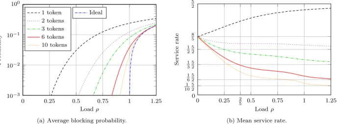
Number of tokens We now focus on the impact of the number of tokens on the performance perceived by the users under dynamic. Figure 11 shows the results.
0 0.25 0.5 0.75 1 1.25 10−3 10−2 10−1 100 Load ρ P ro b a b il it y Ideal 1 token 2 tokens 3 tokens 6 tokens 10 tokens
(a) Average blocking probability.
0 0.25 2 5 0.5 0.75 1 1.25 0 1 10 5 2 1 6 5 2 1 3 5 2 1 2 5 2 8 5 5 2 Load ρ S er v ic e ra te
(b) Mean service rate.
Figure 11: Impact of the number of tokens on the performance of dynamic in the pool of Figure 9. A direct calculation shows that the average blocking probability decreases with the number ℓ of tokens per server, and tends to that obtained under ideal as ℓ → +∞. Intuitively, having many tokens gives a long run feedback on the server loads without blocking the arrivals more than necessary (to preserve stability). Figure 11a shows a semi-log plot of the average blocking probability. The convergence to ideal is quite fast. The small values of ℓ give the largest gain and the performance is already close to ideal with ℓ = 10.
The mean service rate is shown in Figure 11b. As before, it tends to 85 as ρ → 0 and to 1ℓ52 as ρ → +∞. The convergence to 1ℓ52 is all the faster when ℓ increases. Also, a floor emerges between the loads 25 and 1, approximately. This is in line with our previous observation that the effectiveness of dynamic increases when the load exceeds 25.
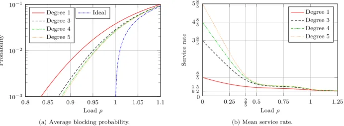
Parallelism degree We finally evaluate the performance improvement when dynamic is combined with some parallel processing. Within each homogeneous part of the pool, r consecutive servers can now process jobs in parallel. A total of 60 tokens are evenly distributed among the classes. Figure 12 shows the results with r = 1, 3, 4, and 5. 0.8 0.85 0.9 0.95 1 1.05 1.1 10−3 10−2 10−1 Load ρ P ro b a b il it y Ideal Degree 1 Degree 3 Degree 4 Degree 5
(a) Average blocking probability.
0 0.25 2 5 0.5 0.75 1 1.25 0 1 6 5 2 8 5 38 5 48 5 58 5 Load ρ S er v ic e ra te Degree 1 Degree 3 Degree 4 Degree 5
(b) Mean service rate.
Figure 12: Impact of the parallelism degree on the performance of dynamic in the pool of Figure 9. The observations are similar to those of the previous paragraph. The average blocking probability is shown in Figure 12a. It decreases with the parallelism degree r, and the largest gain is obtained with small values of r. The mean service rate, shown in Figure 12b, tends to r8
5 when ρ → 0 and to 1 6 5
2 when ρ → +∞.
It is approximately constant between 2 5 and 1.
Overall, these results show that dynamic reaches a good performance, especially when the load is critical, even with a limited number of tokens per server or parallelism degree.
4.3
Several job types
We now consider a pool of S = 10 servers, all with the same unit capacity µ = 1, as shown in Figure 13. As before, each class identifies a unique server that applies PS policy to its jobs and has ℓ = 6 tokens. There are two job types with different arrival rates and compatibilities. Type-1 jobs have a unit arrival rate ν and can be assigned to any of the first seven servers. Type-2 jobs arrive at rate ν
4 and can be assigned to any of
the last seven servers. Thus only four servers can be accessed by both types. Note that heterogeneity now lies in the job arrival rates and not in the server capacities.
µ µ µ µ µ µ µ µ µ µ
ν ν4
Left servers Central servers Right servers
Comparison We again consider two variants of the static load balancing: best static, in which the assign-ment probabilities are chosen so as to homogenize the arrival rates at the servers as far as possible, and uniform static, in which the assignment probabilities are uniform. Note that best static assumes that the arrival rates of the job types are known, while uniform static does not. The results are shown in Figure 14.
Ideal 0 7 10 7 81 3 2 2 3 0 0.2 0.4 0.6 0.8 1 Load ρ O cc u p a n cy ra ti o s Dynamic Best static Uniform static
(a) Average blocking probability (bottom) and resource oc-cupancy (top). 0 7 10 7 81 3 2 2 3 0 1 6 1 4 1 2 3 4 1 Load ρ S er v ic e ra te Dynamic Best static Uniform static
(b) Mean service rate.
0 7 10 7 8 1 3 2 2 3 0 0.2 0.4 0.6 0.8 1 Load ρ P ro b a b il it y Dynamic Best static Uniform static
(c) Probability that each server is idle. Under dynamic and best static, the left and central servers (bottom plot) are idle with the same probability, while the right servers (top plot) are idle with a higher probability. Under uniform static, the central servers (bottom plot) are idle with the lowest probability, followed by the left servers (middle plot) and the right servers (top plot).
Figure 14: Comparison of the insensitive load balancing policies in the pool of Figure 13.
Figure 14a shows the average occupancy ratios. As before, ideal refers to the extreme ratios that comply with the system stability. Regardless of the policy, the slope of the resource occupancy breaks down near the load ρ = 78. The reason is that the left and central servers support at least 45-th of the arrivals with only
7
10-th of the service capacity, so that their effective load is at least 8
7ρ. It follows from (14) that the average
blocking probability in a stable system cannot be less than 45(1 −781ρ) when ρ ≥ 78. Under ideal, the slope of the resource occupancy breaks down again at ρ = 3
2. This is the point where the right servers cannot
support the load of type-2 jobs by themselves anymore. Otherwise, most of the observations of §4.2 are still valid. The performance gain of dynamic compared to best static is maximal near the first critical load ρ = 7
Its delta with ideal is maximal near 78 and 32. Elsewhere, all schemes have a similar performance, except for uniform static that deteriorates faster.
The mean service rate is shown in Figure 14b. Irrespective of the policy, it tends to the unit server capacity as ρ → 0 and to 16 as ρ → +∞. The mean service rate is higher under dynamic than under the static policies when the load is small. Its slope breaks down near ρ = 107, which is also the point where the central servers become overloaded under uniform static.
Figure 14c shows the probability that each server is idle. Under dynamic, that of the left and central servers decreases like 1 − 8
7ρ while that of the right servers decreases like 1 − 2
3ρ. By conservation, this
suggests that the effective load at the left and central servers is 8
7ρ while that at the left servers is 2
3ρ. This is
exactly the load distribution achieved by best static. Interestingly, dynamic succeeds in equalizing the loads at the left and central servers, although these servers have different compatibilities. Also, the effective load
2
3ρ of the right servers can only be so high because type-2 jobs are mostly served by these servers (as long
as ρ < 32), otherwise it would be lower.
Overall, these numerical results show that dynamic often outperforms best static and is close to ideal. The configurations (not shown here) where it was not the case involved very small pools, with job arrival rates and compatibilities opposite to the server capacities. Our intuition is that our algorithm performs better when the pool size or the number of tokens allow for some diversity in the assignments.
Per-type performance We look at two metrics that detail the impact of dynamic on the jobs of each type. The results are shown in Figure 15. For now, we focus on line plots and larger marks which give the performance when job sizes are exponentially distributed with unit mean.
0 7 10 7 81 3 2 2 3 0 0.2 0.4 0.6 0.8 1 Load ρ P ro b a b il it y Average Type-1 jobs Type-2 jobs
(a) Blocking probability of each job type.
Type-1 jobs Type-2 jobs 0 7 10 7 81 3 2 2 3 0 6 12 18 24 30 36 42 Load ρ N u m b er o f jo b
s Left and central servers Right servers
(b) Mean number of jobs of each type.
Figure 15: Performance of dynamic in the pool of Figure 13. Analytical results (line plots) and simulation results (marks). Smaller marks give the results for hyperexponentially distributed sizes. Larger marks, in Figure 15b, give the results for exponentially distributed sizes (because the corresponding metrics cannot be derived from the queueing model).
The blocking probability is shown in Figure 15a. That of type-2 jobs increases near the load ρ = 32. Below this threshold, the right servers can support the load of these jobs by themselves while the left and central servers are mostly occupied by type-1 jobs; beyond this threshold, the right servers become overloaded by type-2 jobs. Note that the blocking probability of type-1 jobs increases earlier, near ρ = 7
8, when the left
and central servers become overloaded by these jobs.
The mean number of jobs of each type is shown in Figure 15b. It is compared to the mean number of jobs at the left and central servers on the one hand and at the right servers on the other hand. The results are consistent with the previous observation. When ρ < 3
2, the mean number of type-1 jobs is approximately
that at the right servers. When ρ > 32, some jobs of type 2 are offloaded towards the central servers while the mean number of type-1 jobs decreases.
(In)sensitivity We also use Figure 15 to evaluate the sensitivity of our algorithm to the job size distribu-tion within each type. Smaller marks give the performance when the job size distribudistribu-tion within each type is hyperexponential: 1
6-th of type-1 jobs have an exponentially distributed size with mean 5 and the other 5
6-th have an exponentially distributed size with mean 1
5; similarly, 1
3-rd of type-2 jobs have an exponentially
distributed size with mean 2 and the other 2
3-rd have an exponentially distributed size with mean 1 2.
The similarity of the results for exponentially and hyperexponentially distributed sizes suggests that in-sensitivity is preserved, even when the job size distribution is type-dependent. Further evaluations, involving other job size distributions and server pool configurations, would be necessary to conclude.
5
Related work on load balancing
We focus on token-based algorithms, such as Join-Idle-Queue (JIQ), in which the load balancer takes the assignment decision based on some state information stored in a local memory. In particular, we do not consider other algorithms, such as join the shortest queue (JSQ) or power-of-d choices, that require instanta-neous communication between the load balancer and the servers upon the job arrival. The interested reader can refer to the survey [17] that compares these approaches in various large-scale regimes.
To the best of our knowledge, our paper is the first to consider a tripartite compatibility graph. In many works about load balancing, the compatibilities are described by a bipartite graph between types and servers (in our model, it means that there is a one-to-one association between servers and classes), and each server has a single token that tells the load balancer whether it is idle. We will refer to this model as the bipartite graph model. As a special case, the supermarket model further assumes that all servers have the same unit service capacity and all incoming jobs can be assigned to any server (in our model, it means that there is a single job type).
5.1
Blocking policies
We first consider policies that reject incoming jobs if no compatible token is available. These policies are insensitive.
Randomized assignment As observed before, our token-based algorithm is a deterministic implementa-tion of the randomized policy introduced in [10]. It is important to note, however, that the perspective we adopted in §3.2 to describe this randomized policy differs from that of [10]. Essentially, our model emphasizes classes: the limits on the number of jobs hold on each class, and the assignment decision is based on the number of jobs within each class. This is what allows us to reduce load balancing to a problem of resource allocation in a network of PS queues. By contrast, most of the results in [10] emphasize types. The focus is on policies in which the decision of assigning a job of a given type to a class only depends on the number of jobs of this type within each class.
The two approaches are equivalent when there is a single job type. This special case was considered in [18] in the supermarket model and its extension to several tokens per server. In particular, [18] studies the asymptotic blocking probability when the number of servers goes to infinity, under various scaling regimes, and numerically compares the performance of the randomized insensitive policy to that of JIQ and JSQ. Deterministic assignment The token-based implementation we propose is deterministic. The closest existing algorithm we know is assign to the longest idle server (ALIS), introduced in [3] for the bipartite graph model. ALIS can be seen as a special case of our algorithm for server pools without parallel processing nor server multitasking. With this simplification, [3] derives simpler formulas for the occupancy ratios introduced in §4.1, and formally proves the insensitivity to the job size distribution at each server, only
assuming that the mean is finite. Just like our algorithm, ALIS is a deterministic implementation of the randomized policy considered in [2] in the bipartite graph model.
5.2
Non-blocking policies
The above-mentioned algorithms, including ours, can be adapted to admit incoming jobs even when no compatible token is available. We distinguish between two cases, depending on whether the assignment decision need be taken upon the job arrival or can be postponed until a compatible token becomes available. This allows us to position our algorithm compared to other non-blocking algorithms such as JIQ. These are not, strictly speaking, insensitive, although insensitivity was shown to hold in the large-scale regime in some cases [19].
Immediate assignment JIQ was first introduced in [19] for the supermarket model. Each server sends its token to the load balancer (or to one of them, if there are several) when it becomes idle. Each incoming job is assigned to the server with the longest available token (that is, to the longest idle server), if any, or to a server chosen uniformly at random otherwise. Supplementing our algorithm with a similar uniform random assignment in the absence of available compatible tokens gives a natural extension of JIQ to our server pool model. Note that the parallel between the blocking and non-blocking versions of JIQ was already drawn in [20] for the supermarket model.
Postponed assignment Alternatively, all incoming jobs that do not find an available compatible token can be stored at the load balancer and assigned to classes later, as tokens are released. An algorithm called FCFS-ALIS, combining FCFS service discipline with the above-mentioned ALIS algorithm, was proposed in [4] for the bipartite graph model: an incoming job is assigned to the longest available compatible server, if any; conversely, when a server becomes idle, it starts to process the longest waiting compatible job. Extending FCFS-ALIS to our server pool model could be the topic of future works.
6
Conclusion
We have introduced a new server pool model that explicitly distinguishes the compatibilities of a job from its actual assignment by the load balancer. Expressing the results of [10] in this new model has allowed us to see the problem of load balancing in a new light. We have derived a deterministic, token-based implementation of a dynamic load balancing policy that preserves the insensitivity of balanced fairness to the job size distribution within each class. Numerical results have assessed the performance of this algorithm. For the future works, we would like to prove the insensitivity of the proposed algorithm to the job size distribution within each type. We are also interested in evaluating its performance in broader classes of server pools, and in particular in better understanding the joint impact of load balancing and resource sharing. Along the same lines, we would like to analyze the performance of various non-blocking extensions.
Acknowledgement The author would like to thank Fabien Mathieu for his help with the proof of irre-ducibility provided in the appendix.
A
Proof of irreducibility
We prove the irreducibility of the Markov process defined by the state (c, d) of the closed tandem network of two OI queues described in §3.3. From now on, we simply refer to this network as the network. The queue of tokens held by jobs in service is called the first queue and the queue of available tokens is called the second queue. These are the two main assumptions we use along the proof:
(P) Positive service rate For each class i ∈ I, we have Ki6= ∅ and Si6= ∅. Also, µs> 0 for each server
(S) Separability For each classes i, j ∈ I with i 6= j, we have Si6= Sj or Ki6= Kj (or both).
Our result is the following: The Markov process defined by the state of the network is irreducible on the state space S = {(c, d) ∈ I∗× I∗: |c| + |d| = ℓ} comprising all states with ℓ
itokens of class i, for each i ∈ I.
The proof is recursive: to connect two arbitrary states, we build a finite series of state transitions that first arrange the tokens of classes 1 to N − 1 and then position the class-N tokens among them. A.1 and A.2 introduce two elementary types of transitions, called circular shift and overtaking, and specify in which states they can occur. These transitions are assembled in A.3 to build finite series of transitions that have the effect of swapping the positions of two consecutive tokens in the queues. Finally, A.4 explains the recursive construction. The proof is illustrated by examples relating to the toy configuration depicted in Figure 16.
1 2 3 4
µ1 µ2 µ3
ν1 ν2
Figure 16: A technically interesting toy configuration. We let s = P
i∈Iℓi denote the number of tokens in the network and T = {t ∈ Is : |t| = ℓ} the set of
sequences obtained by concatenating the states of the two queues in any network state. For each sequence (t1, . . . , ts) ∈ T and integers δ, n = 0, . . . , s, the couple ((tδ+1, . . . , tδ+n), (tδ+n+1, . . . , tδ+s)), where each
index is to be replaced by its residue in {1, . . . , s} modulo s, belongs to S. By convention, the first queue is empty if n = 0 and the second queue is empty if n = s.
A.1
Circular shift
A circular shift, or shift for short, is a transition induced by the service completion of a token at the head of a queue. Consider a state ((c1, . . . , cn), (d1, . . . , dm)) ∈ S. Assuming that n ≥ 1, a shift in the first
queue leads to the state ((c2, . . . , cn), (d1, . . . , dm, c1)). It is triggered by the departure of the oldest job in
the system that releases its token, of class c1, upon service completion. Assumption (P) guarantees that the
rate of this transition, given by P
s∈Sc1µs, is positive. Assuming that m ≥ 1, a shift in the second queue
leads to the state ((c1, . . . , cn, d1), (d2, . . . , dm)). It is triggered by the arrival of a job that seizes the longest
available token, of class d1. Again by Assumption (P), its ratePk∈K
d1νk is positive. Therefore, a shift can
always occur in a non-empty queue.
By the following lemma, two states that are circular shifts of each other belong to the same strongly connected component in the transition diagram of the Markov process defined by the network state. It is illustrated in Figure 17a and 17b.
Lemma 1. Consider a sequence (t1, . . . , ts) ∈ T and three integers δ, n, n′= 0, . . . , s. There is a finite series
of circular shifts that connects the state ((t1, . . . , tn), (tn+1, . . . , ts)) to the state ((tδ+1, . . . , tδ+n′), (tδ+n′+1,
. . . , tδ+s)).
Proof of the lemma. Applying s − n shifts in the second queue leads to the state ((t1, . . . , ts), ∅) in which the
second queue is empty. Now let r denote the remainder of the Euclidean division of δ + n′ by s. Applying r shifts in the first queue and then r shifts in the second queue leads to the state ((tδ+n′+1, . . . , ts, t1, . . . ,
tδ+n′), ∅) in which the token that should eventually be at the head of the second queue is at the head of the
2 1 c = (1, 2) µ1 µ2 µ3 4 1 2 3 4 d = (4, 1, 2, 3, 4) ν1 ν2
(a) An initial state.
4 3 2 1 4 c = (4, 1, 2, 3, 4) µ1 µ2 µ3 1 2 d = (1, 2) ν1 ν2
(b) After a series of shifts.
2 4 3 2 1 4 c = (4, 1, 2, 3, 4, 2) µ1 µ2 µ3 1 d = (1) ν1 ν2
(c) After a class-2 token over-takes its predecessor in the second queue. 1 4 3 c = (3, 4, 1) µ1 µ2 µ3 4 1 2 2 d = (4, 1, 2, 2) ν1 ν2
(d) All tokens of class 2 are gathered at the end of the sec-ond queue.
Figure 17: Application of circular shifts and overtakings.
Hence, we can think of the network state as a ring obtained by attaching the head of each queue to the tail of the other queue. We now describe transitions that have the effect of swapping the positions of two consecutive tokens in this ring.
A.2
Overtaking
An overtaking is a transition induced by the service completion of a token in the second position of a queue. We also say that this token overtakes its predecessor in the queue. Unlike a shift, an overtaking cannot happen in any state (in general) because the service rate of the token in the second position may be zero. Consider a state ((c1, . . . , cn), (d1, . . . , dm)) ∈ S. If n ≥ 2, an overtaking in the first queue leads to the
state ((c1, c3, . . . , cn), (d1, . . . , dm, c2)). It is possible if and only if Sc2 * Sc1, meaning that there is at
least one server that can can process the job holding the class-c2 token but not the job holding the class-c1
token. Indeed, the rate of this transition isP
s∈Sc2\Sc1µs, and Assumption (P) guarantees that µs> 0 for
each s ∈ S. Symmetrically, if m ≥ 2, an overtaking in the second queue leads to the state ((c1, . . . , cn, d2),
(d1, d3, . . . , dm)) and is possible if and only if Kd2 * Kd1, meaning that there is at least one job type that
can seize the class-d2 token but not the class-d1 token.
We now combine Assumption (S) with a structural argument on the server and type sets to prove the following lemma. The steps of this proof are illustrated in Figure 18.
Lemma 2. By renumbering the classes if necessary, we can work on the assumption that, for each i = 2, . . . , N and each j = 1, . . . , i − 1, a class-i token can overtake a class-j token in (at least) one of the two queues.
Proof. We first sort the distinct servers sets, Si, i ∈ I, in an order that is non-decreasing for the inclusion
relation on the power set of {1, . . . , S}. In other words, we consider a topological ordering of these sets induced by their Hasse diagram, so that a given server set is not a subset of any server set with a lower rank. Therefore, a token of a class whose server set has a given rank can overtake, in the first queue, a token of any class whose server set has a lower rank, but not a token of a class whose server set is identical.
We also sort the distinct type sets Ki, i ∈ I, in an order that is non-decreasing for the inclusion relation
on the power set of {1, . . . , K}, so that a given type set is not a subset of any type set with a lower rank. Again, a token of a class whose type set has a given rank can overtake, in the second queue, a token of any class whose type set has a lower rank, but not a token of a class whose type set is identical.
Using these orders on the server and type sets, we sort and renumber the token classes as follows. We first order the classes having distinct server sets by increasing server set rank, and then we order the classes sharing the same server set by increasing type set rank. Assumption (S) guarantees that two distinct classes are indeed ordered. With this new numbering, for each i = 2, . . . , N and each j = 1, . . . , i − 1, a class-i token can overtake a class-j token in the first queue (if these classes have different server sets) or in the second queue.