Multidimensional Hidden Markov Model Applied to Image and Video Analysis

HAL Id: pastel-00002454

https://pastel.archives-ouvertes.fr/pastel-00002454

HAL is a multi-disciplinary open access archive for the deposit and dissemination of sci-entific research documents, whether they are pub-lished or not. The documents may come from teaching and research institutions in France or abroad, or from public or private research centers.

L’archive ouverte pluridisciplinaire HAL, est destinée au dépôt et à la diffusion de documents scientifiques de niveau recherche, publiés ou non, émanant des établissements d’enseignement et de recherche français ou étrangers, des laboratoires publics ou privés.

To cite this version:

Joakim Jitén Söderberg. Multidimensional Hidden Markov Model Applied to Image and Video Anal-ysis. domain_other. Télécom ParisTech, 2007. English. �pastel-00002454�

Multidimensional Hidden Markov Model

Applied to Image and Video Analysis

by

Joakim Jitén Söderberg

A Thesis Submitted to the Graduate Faculty of Ecole Nationale Supérieure des Télécommunications Paris

in Partial Fulfillment of the Requirements for the degree of

DOCTOR OF PHILOSOPHY Major Subject: Signal and Images

Approved by the Examining Committee:

_________________________________________ Bernard Merialdo, Thesis Adviser

_________________________________________ Georges Quenot, Opponent

_________________________________________ Pierre Courtellemont, Opponent

_________________________________________ Gaël Richard, Member

_________________________________________ Gerhard Rigoll, Member

_________________________________________ Philippe Joly, Member

Institute Eurecom Sophia Antipolis

© Copyright 2007 by

Institute Eurecom All Rights Reserved

Author’s address: Joakim Jitén joakim.jiten@eurecom.fr B.P. 193 06904 Sophia-Antipolis France

iii

ABSTRACT

Recent progress and prospects in cognitive vision, multimedia, human-computer interaction, communications and the Web call for, and can profit from applications of advanced image and video analysis. Adaptive robust systems are required for analy-sis, indexing and summarization of large amounts of audio-visual data.

Image classification is perhaps the most important part of digital image analysis. The objective is to identify and portray the visual features occurring in an image in terms of differentiated classes or themes. Applications can be found in a wide range of domains such as medical image understanding, surveillance applications, remote sensing and interactive TV.

Traditional image classification methods analyses independent blocks of an image, which results in a context-free formalism. However there is a fairly wide-spread agreement that observations should be presented as collections of features which appear in a given mutual position or shape (e.g. sun in the sky, sky above landscape or boat in the water etc.) [20], [21]. Consider analyzing local features in a small region of an image; it is sometimes difficult even for a human to tell what the image is about.

In this dissertation we apply a statistical machine learning approach to model context in sequential data. With a statistical model in hand, we can perform several important tasks to image analysis such as; estimation, classification and segmentation.

We employ a new efficient algorithm that models images by a two dimensional hidden Markov model (HMM). The HMM considers observations statistically dependent on neighboring observations through transition probabilities organized in a Markov mesh, giving a dependency in two dimensions. The main difficulty with applying a 2-D HMM to images is the computational complexity which grows exponentially with the number of image blocks.

The main technical contribution of this thesis is a way of estimating the parameters of a 2-D HMM in O(whN2) complexity instead of O(wN2h), where N is the number of states in the model and (w,h) is the width respectively height of the image.

iv

We investigate the performance of our proposed model (DT HMM), and search for its point of operation. Application to classification of TV broadcast frames reveal intrinsic weaknesses of the HMMs for which we propose remedies.

In an effort to introduce both global and local context in images, the DT HMM was extended to model multiple image resolutions. The results indicate that the earlier recorded deficiency can be conquered and that its performance can be compared with other known algorithms.

Finally we illustrate that the DT HMM formalism is open to a great variety of extensions and tracks. Since 3-D HMMs has been little studied we investigate the extension of the framework to three dimensions. We consider the case of video data, where the two dimensions are spatial, while the third dimension is temporal. To investigate the impact of the time-dimension dependency we explore the ability of the model to track objects that cross each other or pass behind another static object.

v

RÉSUMÉ

Les progrès récents dans les domaines de la vision cognitive, du multimédia, de l'interaction homme-machine, des communications et de l’Internet sont un apport considérable pour la recherche qui profite à l’imagerie et l’analyse vidéo. Des systèmes adaptés et fiables sont nécessaires pour l’analyse, l’indexation et le résumé de grandes quantités de données audiovisuelles.

La classification d’images constitue sans doute, la partie la plus importante de l’analyse de l’image numérique. L’objectif est d’identifier et de décrire les caractéris-tiques présentes dans une image afin de les répertorier par classes et par thèmes. Des applications existent dans un grand nombre de domaines, tels que l’interprétation de l’imagerie médicale, la surveillance, la photo satellite et la télévision interactive. Les méthodes traditionnelles de classification d’images procèdent par analyse des blocs distincts d’une image, ce qui aboutit à un formalisme non contextuel des caractéristiques visuelles. Toutefois, face à l’analyse d’une parcelle d’image, l’œil humain est souvent dans l’incapacité d’identifier ce qu’il voit. Les approches récen-tes tendent donc de plus en plus vers une vision globale de l’image incluant sa structure et sa forme générale (ex: le soleil dans le ciel, le ciel au dessus d’un paysage ou encore un bateau sur l’eau, etc.) [20], [21].

HMM Multi dimensionnel

Cette thèse est une approche statistique issue de l’intelligence artificielle visant à une représentation séquentielle des données de l’image. Cette représentation statistique permet l’estimation, la classification, et la segmentation de l’image.

Nous utilisons un nouvel algorithme efficace représentant les images à l’aide du modèle bidimensionnel de Markov caché (HMM). Le HMM considère les observa-tions statistiquement dépendantes d’observaobserva-tions voisines à travers des probabilités de transition organisées dans les mailles de Markov, ce qui induit une dépendance en deux dimensions. La principale difficulté à appliquer un 2-D HMM aux images est la

vi

complexité algorithmique qui s’accroît de façon exponentielle avec le nombre de segments d’image.

En conséquence, la contribution technique majeure de cette thèse est d’estimer les paramètres d’un nouveau type de 2-D HMM dont la complexité sera O(LlN2) au lieu de O(LN2l) où N est le nombre d’états dans le modèle et (L,l) sont respectivement la largeur et la longueur de l’image.

Modèle d’entraînement

L’algorithme EM est généralement employé pour trouver l’estimation des paramètres du modèle de Markov caché la plus probable d’après les vecteurs caractéristiques observés. Cet algorithme est aussi connu sous le nom d’algorithme de Baum-Welch. Nous décrivons l’ensemble complet des paramètres pour un modèle donné par λ = (aij, bs(ot), πs). Comme montré en [37], trois problèmes fondamentaux doivent être

résolus pour l’utilisation des HMMs.

Problème 1: Estimer P(O|λ), La probabilité de la séquence d’observation selon les paramètres du modèle

Problème 2: Trouver la séquence d’états S = {s1,…,sT} la plus significative.

Problème 3: Comment ajuster les paramètres du modèle λ* _{pour maximiser P(O|λ)?}

Comme nous verrons dans la section 3.1, il y a des méthodes établies pour travailler sur ces problèmes. Ce sont respectivement les algorithmes « forward-backward », de Viterbi, et de Baum-Welch. Dans la section suivante, Je montrerai que ces algorith-mes peuvent être adaptés au nouveau modèle proposé.

Extensions 2-D nécessaires pour la classification d’images

Nous divisons une image en une grille régulière de blocs. Un bloc est désigné par sa position (i,j), et l’ensemble complet des blocs est ℵ = { (i,j): 0≤i<L, 0≤j<l }où L et l sont respectivement la largeur et la hauteur de l’image. Un vecteur caractéristique oij

est calculé pour chaque bloc (i,j) et l’ensemble de vecteurs caractéristiques O = {oij :

(i,j) ∈ ℵ } décrivant l’image entière est appelée « champ de vecteurs ». D’après les hypothèses des 2-D HMM, ce champ de vecteurs est généré par les états du modèle. L’image est donc classée en accord avec ses vecteurs caractéristiques.

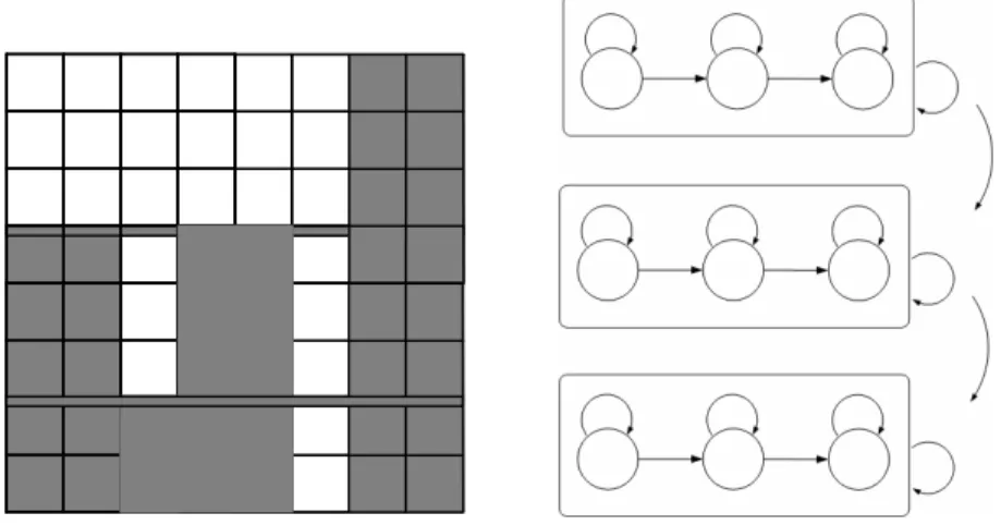
Un 2-D HMM est une grille de noeuds, chacun correspondant à un bloc. A Chaque nœud peut être affecté un des N états possibles {1,2,…,N}. L’état d’un bloc (i,j) est noté sij. La Figure 1 illustre les blocs d’une image ainsi que les nœuds

vii

Figure 1. (a) Décomposition de l’image en blocs, (b) Etats du modèle de Markov La formalisation du 2-D HMM est basée sur deux hypothèses. La première est :

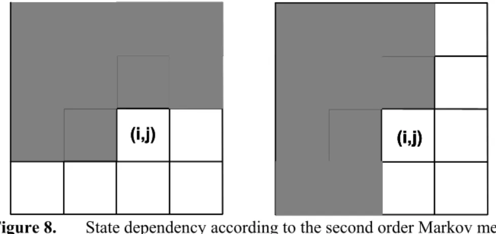
l n m j i j i j i s o i j a s P( _, | _{,' '}, _{,' '}:( ,' ')∈Ψ)= _{, ,} where Ψ={(i,'j'):(i'j')<(i,j)} and m=s_i−_1,j,n=s_i,j−₁,l =s_i,j (1.1)

Cela signifie que le processus d’états est Markovien du premier ordre: La probabilité que le système entre dans un état particulier à la position (i,j) dépend uniquement des états des observations adjacentes selon les directions horizontales (i-1,j) et verticales (i,j-1). La deuxième hypothèse stipule que le vecteur caractéristique est seulement dépendant de l’état à la position (i,j), i.e. l’observation est conditionnellement indé-pendante des autres blocs.

Comme précédemment, nous noterons par λ les paramètres du HMM, donc selon les hypothèses de Markov, la probabilité conjointe de O et S selon λ peut être calculée d’après :

(

) (

)

∏

Notons que la probabilité conditionnelle P(si,j|si,j-a,si-1,j,λ) se réduit à P(s1,j|s1,j-a,λ)

lorsque i=1, à P(si,1|si-1,1,λ) quand j=1, et à P(s1,1| λ) si i=j=1.

Dans la section suivante, nous présenterons une méthode efficace pour calculer P(O,S|λ) basée sur l’idée d’un arbre de dépendances aléatoires.

Arbre de dépendance

Comme mentionné précédemment, le problème avec les 2-D HMM est la double dépendance entre si,j et ses deux voisins si-1,j et si,j-1, qui n’autorise pas la

viii

(i-1,j)

(i,j-1) (i,j)

Figure 2. Voisins 2-D

Notre idée suppose que si,j dépend uniquement d’un voisin à la fois. Ce voisin peut

être celui à son horizontale ou à sa verticale, selon une variable aléatoire t(i,j). Plus précisément, t(i,j) est susceptible de prendre deux valeurs distinctes:

⎩ ⎨ ⎧ − − = 5 0 prob with 1 j i 5 0 prob with j 1 i j i t . ) , ( . ) , ( ) , ( (1.3)

Pour la position sur la première ligne ou la première colonne, t(i,j) a seulement une seule valeur, celle qui conduit à une position valide dans le domaine. t0,0) n’est pas défini. Ce qui induit les simplifications suivantes pour notre modèle :

⎪⎩ ⎪ ⎨ ⎧ − = − = = − − − − ) 1 , ( ) , ( ) ( ) , 1 ( ) , ( ) ( ) , , ( 1 , , , 1 , 1 , , 1 , j i j i t if s s p j i j i t if s s p t s s s p j i j i H j i j i V j i j i j i (1.4)

Si nous définissons ensuite une fonction de direction :

⎩ ⎨ ⎧ − = − = = ) , ( ) , ( ) ( 1 j i t if H j 1 i t if V t D (1.5)

Nous obtenons alors la formulation simplifiée :

) ( ) , , (s_i,j s_i1,j s_i,j1 t P_D(t(i,j)) s_i,j s_t(i,j) P − − = (1.6)

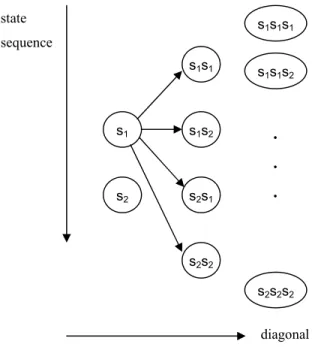
Notons que le vecteur t des valeurs t(i,j), pour tout (i,j) défini une structure d’arbre sur l’ensemble des positions, admettant (0,0) comme racine. La Figure 3 montre un exemple d’arbre de dépendances aléatoires

ix

Figure 3. Exemple d’arbre de dépendances aléatoires.

Avec cette structure d’arbre, nous pouvons calculer la probabilité d’une observation produite par le modèle quelque soit la séquence d’état (tant que les états sont incon-nus).

∑

Et la séquence d’état la plus probable s* qui génère ce résultat :

) | , ( max arg P o s t s (1.8)

Nous allons maintenant montrer comment résoudre un des trois problèmes fonda-mentaux cités en 2.4.9, ce qui nous permettra de mesurer le score d’une observation selon le modèle λ.

Solution au Problème 1, estimer P(O|

λ)

Nous voulons calculer la probabilité de l’observation en fonction des paramètres P(O|λ) (2.1). Nous définissons la probabilité intérieure βij(s) comme la probabilité

que la partie de l’image couverte par le sous arbre T(i,j) de racine (i,j) soit produit par la séquence d’observation partielle et se termine à la position (i,j) (voir la portion ombrée sur la Figure 4).

x

Figure 4. Les probabilités intérieures

Ces valeurs peuvent être calculées récursivement, dans l’ordre inverse (en par-tant de la dernière position) de leurs relations :

• Si (i,j) est une feuille de t(i,j) :

) ( ) ( , ,j s poijs i = β (1.9)

• Si (i,j) admet seulement un successeur horizontal : ) ' ( ) ' ( ) ( ) ( , ' , , s po s p s s ij1 s s H j i j i =

∑

• Si (i,j) a seulement un successeur vertical :

) ' ( ) ' ( ) ( ) ( , ' , , s po s p s s i 1j s s V j i j i =

∑

• Si (i,j) a deux successeurs, l’un horizontal et l’autre vertical :

⎟ ⎟ ⎠ ⎞ ⎜ ⎜ ⎝ ⎛ ⎟ ⎟ ⎠ ⎞ ⎜ ⎜ ⎝ ⎛ = + +

∑

∑

xi ) ( ) (O t _0,0 s_i P =β (1.13)

ce qui nous donne la solution au problème. La problématique 1 est applicable dans le domaine de la classification où l’on veut choisir un modèle qui satisfait le mieux une observation.

Expériences

Dans notre première expérience, nous utilisons l’arbre de dépendance HMM en temps que structure pour un classificateur d’images contextuel. Nous explorons aussi comment l’équilibre entre l’information structurelle et le contenu descriptif affectent la précision et le rappel en variant la taille des blocs.

Les algorithmes Baum-Welch modifiés (voir la section 3.4) ont été utilisés pour évaluer les paramètres des modèles dans la phase expérimentale. Pour classifier une image, ses descripteurs de bas niveau sont extraits et ensuite P (O | λ) est calculé pour chaque modèle évaluant le niveau de correspondance entre le modèle et l'obser-vation, puis on recherche ensuite le modèle fournissant la plus haute probabilité a posteriori. On montre une illustration générale du système de classification dans la Figure 5. feature extraction block description HMM training feature extraction block description HMM classification training image training feature

test image test feature result

block size

Figure 5. Schéma de Catégorisation d'Image.

Le graphique ci-dessous montre la précision de classification moyenne pour sept tailles de bloc différentes. Nous avons remarqué qu'une taille de bloc de 16x15 pixels ( modèle #4) donne la précision moyenne la plus haute 0.036.

xii

Figure 6. La précision moyenne pour tailles de bloc: (1) 176x120, (2) 88x60, (3) 44x40, (4) 16x15, (5) 8x8, (6) 4x4, (7) 2x2

Nous pouvons aussi voir que la performance diminue rapidement avec de très grands blocs. L'explication est que les moyennes des canaux de couleur ne sont pas assez descriptives et que les coefficients DCT refléteront seulement des hautes variations de fréquence puisque l'échelle sera plus haute quand la taille de bloc est augmentée. Les résultats ne sont pas comparables avec les taux typiquement observés dans les expériences vidéo TREC [66], cependant ils nous mènent à une compréhension plus grande du modèle et ont inspiré de nouvelles expériences et raffinements qui seront discutés dans les chapitres suivants.

Nous avons noté un inconvénient connu du HMM: la probabilité de production joue un rôle plus important que la probabilité de transition. La sortie de distribution s'étend sur la plus grande dispersion que sur la probabilité de transition (cette derniè-re s'étend sur 16 états seulement), avec une majorité de transitions d'un état à l’autre.

Cela explique pourquoi une image qui a une couleur presque uniforme a une haute probabilité d'émission.

Influence de l'Arbre de Dépendance

Le DT HMM est rendu moins complexe que le 2-D HMM, en changeant les dépen-dances spatiales horizontales et verticales doubles en une dépendance unidirectionnelle aléatoire, horizontale ou verticale. La question qui se pose est: quel l'impact ce choix aléatoire a-t-il sur le modèle? Nous explorons donc les différents aboutissements de l'effet de l'arbre aléatoire.

Selon le modèle, la probabilité exacte d'une observation est :

∑

Model# (block size)

16x15 R-precision 50precision random precision

xiii

Nous pouvons postuler qu'il faut une équivalence de tous les arbres de dépendance,

pour que la distribution P(t) soit uniforme. Étant donné qu'il y a ₂(m−1)(n−1) _arbres différents pour une image de blocs m x n, le calcul complet est prohibitif. Donc, il est important de chercher des approximations de cette valeur qui sont faciles à calculer. À cette fin nous examinons trois façons différentes de faire cette évaluation par: prélèvement d'échantillon unique (Pu), moyenne d'arbre (Pa) et arbre dual (Pd). La Section 3.8 donne une étude détaillée de leurs qualités.

Segmentation sémantique d’images

Pour mieux évaluer les possibilités du modèle, nous avons introduit un champ

interprétation aux états du DT HMM en associant une sous-classe pour partitionner

les états. Affecter plusieurs états par sous-classe donne au modèle la flexibilité suffisante pour s’adapter aux sous–classes ayant des observations visuelles variées. En entraînant un nouveau modèle avec des états restreints, nous pouvons effectuer une segmentation sémantique de l’image sur des données non connues pourvu qu’elles appartiennent à une des classes.

Etats pourvus d’un label sémantique

A chaque sous-classe est assignée un ensemble d’états pour permettre une représenta-tion flexible. Supposons qu’il y ait K sous-classes (1,…,K) et qu’un vecteur d’observation oij appartienne à une région annotée avec une sous-classe ck. Alors, son

ensemble d’états permis est {s(k)}. La table ci-dessous liste les différentes sous-classes et leur nombre d’états alloués.

Table1. Nombre d’etats pour chaque classe.

Sous Classe No. d’état

Divers 3 Ciel 7 Mer 5 Sable 6 Montagne 3 Végétation 3 Personne 4 Batiment 3 Bateau 2 9 sous-classes 36 états

Nous utilisons une version modifiée de l’algorithme de Viterbi capable de gérer la situation lorsqu’une sous-classe visuelle est représentée par plusieurs états, et que seules les annotations des sous-classes sont disponibles. Nous avons étudié plusieurs propriétés de ce procédé.

xiv

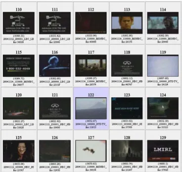
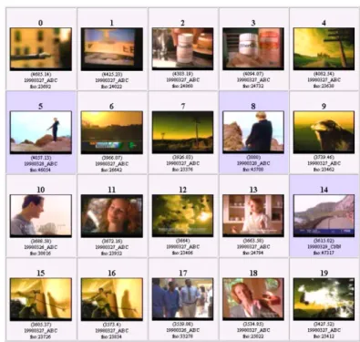
L’entraînement fut effectué sur les archives de TRECVid [66], duquel nous avons tiré une collection hétérogène de 130 images dépeignant « plage » (voir Figure dessous).

Figure 7. Examples d'Images entraînement.

L’expérience fut conduite sur 40 images tests sémantiquement segmentées. Nous avons comparé la meilleure affectation d’état obtenue par l’algorithme de Viterbi (Cela prend en compte à la fois les probabilités de sortie et de transition) avec l’affectation où chaque vecteur caractéristique est associé à l’état de meilleure probabilité de sortie. Le taux moyen de blocs correctement labellisés est de 38% en prenant en compte les probabilités de transition, et de 32% pour les probabilités de sortie seules.

La table de confusion ci-dessous montre le nombre de blocs classés pour chaque classe. On constate que Ciel est parfois confondu avec sable (à cause des réflexions,

comme dans Figure 43 b). De même, on note l’amalgame occasionnel de mer avec

sable (à cause de leur recouvrement), et de montagne avec sable (du à leurs

descrip-teurs similaires). Les classes végétation, bâtiment, et bateaux, sont faibles à cause du manque d’images d’entraînement.

Table 2. Table de confusion.

Annotées

Classées divers ciel mer sable mont veg pers bat bateau

divers 0 0 0 0 0 0 0 0 0 ciel 199 1470 636 228 59 4 115 50 21 mer 382 136 1090 314 168 28 89 165 66 sable 245 677 573 1008 452 24 181 152 51 montagne 101 66 120 86 73 14 31 94 24 végétation 84 84 42 183 98 95 17 45 7 personne 305 260 287 601 271 145 601 196 128 bâtiment 54 11 62 90 24 7 33 57 20 bateau 2 15 2 2 0 0 1 1 2

L’exemple suivant montre quelques images segmentées, ainsi que leur nombre de blocs convenablement classés

xv

Figure 8. Exemple d’images segmentées.

a) 72% correctement classés

b) 28% correctement classés

xvi

Modèle de Markov Caché Multi résolution

Dans l’expérience précédente, nous avons démontré qu’une importante probabilité de sortie dégrade les résultats, mais aussi que le modèle contextuel échoue parfois à caractériser les sous-classes d’un concept, ce qui suggère une échelle trop petite. D’une part, une échelle élevée est nécessaire afin de distinguer les détails des objets, et d’autre part, une faible échelle permet de capturer les propriétés globales. Cela amène l’idée du développement d’un modèle multi résolution.

Le principe de l’analyse multi résolution est de capturer l’information d’une image à différentes résolutions. Nous considérons donc une combinaison linéaire de 2-D HMMs entraînés à différentes résolutions. Comparé à la modélisation hiérarchi-que, cette approche est plus aisée à construire: Il nous suffit d’entraîner un certain nombre de 2-D HMMs à différentes résolutions et de les combiner par interpolation ou par probabilité jointe. L’architecture d’un système multi résolution est présentée ci-dessous.

Figure 9. Combinaison linéaire de modèles multi résolution.

Expérience

Pour évaluer les performances de notre modèle, nous le comparons avec le modèle proposé par Jia Li et Al.[39], utilisant le même scénario de classification d’images que dans le chapitre précédent. Les modèles sont entraînés à l’aide d’un ensemble images annotées. La classification est ensuite effectuée sur un ensemble inconnu que le procédé convertit en une liste triée.

m0 m1 m2 mn - λ0 λ1 λn - P( I | m0) P( I | mn)

xvii feature extraction block description HMM training feature extraction block description HMM classification training image training feature

test image test feature result

number of blocks multiple resolutions

Figure 10. Schéma de classification multi résolution.

En redéfinissant itérativement la taille de l’image, tout en conservant la taille du block constante, nous obtenons les résolutions d’images de (a) 4x3, (b) 16x12 et (c) 64x48 blocks, comme illustré ci-dessous.

Figure 11. Trois résolutions avec des tailles de blocks constantes: (a) 4x3, (b) 16x12 et (c) 64x48 blocks.

Les modèles sont entraînés à l’aide des algorithmes adaptés de Baum-Welch, comme décrit dans la section 2.4. La Figure 12 montre l’évolution de la probabilité totale pour le DT-MHMM durant l’entraînement.

-700 -690 -680 -670 -660 -650 -640 -630 -620 -610 -600 0 5 10 15 20 25 Avg. probability Iterations Resolution 0 Resolution 1 Resolution 2

xviii

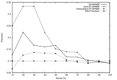
La Figure 13 montre la courbe rappel précision pour le modèle 2-D MHMM (Jia Li et al) et les deux modèles DT-MHMM.

0.05 0.1 0.15 0.2 0.25 0.3 0.35 10 20 30 40 50 60 70 80 90 100 Precision Recall (%) 2D-MHMM Joint DT-MHMM Interpolated DT-MHMM Rdm Precision

Figure 13. Rappel précision pour 2D-MHMM et DT-MHMM.

On peut observer que le modèle introduit à la plus basse résolution une information globale qui pénalise les images mono-couleurs, mais, selon le schéma de fusion, les modèles de plus hautes résolutions rétablissent parfois l’ensemble. La précision moyenne pour les différents modèles est listée en table 3.

Table 3. Précion moyenne pour DT HMM et 2-D MHMM.

Modèle CARTE

DT MHMM combine jointe 0.24

2-D MHMM 0.17

DT MHMM Interpolatée 0.13

Conclusion

Dans le but d’introduire le contexte local et global, le DT HMM est utilisé comme un modèle d’image de multi résolutions. Le résultat indique que la perte enregistrée peut être diminuée et que les performances sont comparables avec celles des autres algorithmes.

xix

Applications 3-D

Enfin nous présenterons les possibilités d’extensions de la formalisation DT HMM par une étude du 3-D HMM (qui a été rarement étudiée). Nous nous focaliserons sur les données vidéo [66], où les deux premières dimensions sont spatiales, et la troi-sième temporelle. Pour mieux comprendre cette dernière dimension, nous explorerons les capacités du modèle dans le domaine du suivi d’objets.

En trois dimensions, l’état si,j,k du modèle dépendra de ces trois voisins si-1,j,k, si,j-1,k,

si,j,k-1. Cette triple dépendance accroît le nombre de probabilités de transition dans le

modèle, et la complexité algorithmique des algorithmes tels que Viterbi ou Baum-Welch. Cependant, l’utilisation d’un arbre de dépendance 3-D nous permet d’estimer les paramètres du modèle le long d’un chemin 3-D (voir Figure 14) qui maintient une complexité algorithmique linéaire.

Figure 14. Arbre de dépendance 3-D aléatoire. La fonction de direction pour l’arbre 3-D devient :

⎪⎩ ⎪ ⎨ ⎧ − = − = − = = ) 1 , , ( ) , 1 , ( 1, , ) ( ) ( k j i t if Z k j i t if H if t i j k V t D (1.15)

En modélisation 3-D, les images sont représentées par des vecteurs caractéristiques sur une grille 3-D. Notons le vecteur d’observation oijk comme l’observation du bloc

(i,j,k) dans une image 3-D, volume d’images issues d’une séquence 2-D. Par analo-gie, les variables d’états sijk du HMM représentent les états aux positions (i,j,k)

produisant les vecteurs d’observation oijk. Nous pouvons donc maintenant étendre

xx

)

(

)

,

,

(

s

s

p

t

s

s

s

s

p

=

Le procédé de suivi se décompose principalement en deux phases : La phase d’entraînement et la phase de segmentation. Lors de la phase d’entraînement, le processus apprend les paramètres inconnus du HMM, à l’aide du système d’entraînement de Viterbi détaillé en section 5.2.1. Au cours de la phase de segmen-tation, le procédé effectue une segmentation spatio-temporelle en exécutant un alignement d’états 3-D de Viterbi.

Détection d'Objet

La vidéo originale contient deux skieurs passant devant des repères jaunes sur un paysage neigeux avec des ombres. Figure 15 retrace chaque seconde de la séquence.

Figure 15. La séquence vidéo commence au coin supérieur gauche, suivi des autres cadres.

Les deux premières images ont été manuellement annotées et utilisées pour évaluer le modèle initial, tandis que les images suivantes constituent l'observation 3-D sur laquelle l’expérience de Viterbi a été exécutée. Puis, nous utilisons le modèle formé pour obtenir un étiquetage finalisé de l'observation 3D complète. Dans l'étiquetage final, chaque bloc d'observation est assigné à un seul état du modèle. L'étiquetage final fournit une segmentation spatio-temporelle de l'observation 3D.

Le dépistage d'objet est alors exécuté facilement, en choisissant dans chaque image les blocs que l'on étiquette en fonction de la catégorie sémantique correspondante.

xxi

Par exemple, nous pouvons facilement créer une séquence vidéo contenant seulement les skieurs en excluant le paysage - et les marques repères comme indiqué ci-dessous.

Figure 16. Détection de deux skieurs.

Nous pouvons voir dans la figure ci-dessus que certains blocs ne sont pas correcte-ment assignés aux catégories de skieur. L'explication peut être qu'avec un seul arbre de dépendance, beaucoup de blocs à l'intérieur de la vidéo correspondent à des feuilles dans l'arbre et sont donc dispersés. Cela justifie la combinaison de plusieurs arbres de dépendance pour que la chaine d'images ne soit pas rompue.

Pour chaque arbre de dépendance, nous pouvons calculer le meilleur alignement, utiliser ensuite un vote majoritaire pour choisir l’état le plus probable pour chaque bloc. C'est une approximation pour la probabilité d'être dans cet état pour ce bloc pendant la génération de l'observation avec un arbre aléatoire inconnu. Figure 17 montre la vidéo obtenue avec cet étiquetage d'arbre multiple, en utilisant un jeu de 50 arbres aléatoirement produits.

xxii

Comme le montrent ces résultats, les objets sont très clairement définis dans cette expérience et la plupart des interférences dans l'étiquetage ont disparues.

Enfin nous avons illustré l'approche DT HMM sur le problème de la segmentation vidéo et de la détection. Nous avons détaillé l'application de notre modèle sur un exemple concret. Nous avons aussi montré que quelques artefacts en raison de nos simplifications peuvent être énormément réduits par l'utilisation d'un plus grand nombre d'arbres de dépendance.

Conclusion et Travail Futur

Grace aux nouvelles capacités d'apprentissage de HMM, nous croyons que ce type de modèle sera appelé à être utilisé pour nombre d'applications. On peut envisager d'autres applications 3-D telles que la classification d'images 3-D ou la reconstruction d'image.

Au delà, puisque l'arbre de dépendance présente des discontinuités nous pouvons trouver d'autres façons de choisir un arbre. Faire par exemple un arbre optimal pour un jeu d'images ou application en analysant d'abord chaque image et faire plus de rapports (connexions) entre des régions de frontière, ou considérer d'autres arbres non-aléatoires.

Une future approche du problème de discontinuités est d'utiliser des modèles hiérar-chiques, puisqu'un bloc dans une résolution plus basse peut inclure les rapports (connexions) qui n'existent pas à plus petite échelle.

Le modèle peut aussi être appliqué (étendu) aux dimensions supérieures (n > 3). Dans ce cas les rapports contextuels deviennent alors plus faibles et pour chaque dimension nous aurons un rapport (connexion)proche de n. Pour cette raison le choix de l'arbre deviendra encore plus important.

En conclusion nous croyons que le DT HMM est un modèle puissant qui a un vérita-ble potentiel d'avenir pour de nombreuses applications.

xxiii

ACKNOWLEDGMENT

This thesis is the result of three and a half years effort spent at the Multimedia Communications Department of institute Eurecom, which has provided me with enriching industrial and academic experiences.

First of all, I would like to thank my principal advisor, Professor Bernard Merialdo, for his great guidance, support and patience. The weekly meetings have greatly helped in developing my work. He has provided me not only with technical and mathematical knowledge but also a rigorous attitude towards research, for which I am grateful. I also express my gratitude to assistant Professor Benoit Huet, for having many discussions with me in machine learning and image processing.

Some people have given me invaluable help and scientific support during my thesis, among them I would like to express all my gratitude to Vivek Tyagi and Fabrice Souvannavong whose resourcefulness has given me the opportunity to learn and explore different subjects related to signal processing, probability theory and pro-gram construction. Special thanks go to Fabio Valente for helping me during the initial part of my PhD.

During my stay at the Eurecom institute, I came across some very special people that I consider friends rather than colleagues: Gwenael, Brian, Federico, Eric, Remi and Rachid. Thank you guys for everything!

Finally I would like to thank the staff at Eurecom for their help with administrative work, and Carole for giving me her remarkable support.

xxiv

xxv

CONTENTS

1.1 Motivation...1 1.2 Contribution and Outline ...2 2.1 Image Understanding ...5

2.1.1 The Meaning of the Picture and Ontologies ...6 2.1.2 Hyponomic Ontology...6 2.1.3 Meronomic Ontology...7 2.1.4 Notes from Cognitive Psychology ...8 2.2 Knowledge Representation and Control Strategy...8 2.3 Applications ...9 2.4 Statistical Learning ...12 2.4.1 Concept Learning...12 2.4.2 Classification Algorithms ...13 2.4.3 Bayesian Classifier...14 2.4.4 Gaussian Mixture Model...16 2.4.5 Naive Bayesian Classifier ...21 2.4.6 Dynamic Bayesian Nets ...21 2.4.7 Hidden Markov Model...22 2.4.8 HMM and Image Modeling ...23 2.4.9 Reestimation Formulas ...24 2.5 2-D HMM ...27

xxvi

2.5.1 Necessary 2-D Extensions for Image Classification...28 2.5.2 Markov Random Field ...29 2.5.3 Markov Mesh Random Field ...31 2.5.4 Previous Work on 2-D HMM ...33 3.1 Dependency Tree ...40 3.2 Solution to Problem 1 (Evaluation Problem) ...42 3.3 Solution to Problem 2 (Decoding Problem)...43 3.4 Solution to Problem 3 (Learning Problem)...44 3.5 Implementation Issues for HMMs ...49 3.6 Experiment ...50

3.6.1 Context Dependent Image Categorization ...50 3.6.2 System Design...51 3.6.3 Extracted Low-Level Features ...52 3.6.4 The Dataset ...53 3.6.5 Results...54 3.6.6 Conclusion ...57 3.7 Combination with a Global Model...58

3.7.1 Vector Quantization ...58 3.7.2 Global Model ...60 3.7.3 Results...60 3.7.4 Conclusion ...63 3.8 Influence of the Dependency Tree ...64

3.8.1 DT HMM Probability Estimation ...64 3.8.2 Estimation by Average...65 3.8.3 Estimation by unique sampling...66 3.8.4 Estimation with dual tree ...67 3.8.5 Conclusion ...68 4.1 Semantic Image Segmentation...69

xxvii

4.1.1 Related Work ...70 4.1.2 Semantic Segmentation...70 4.1.3 States with semantic labels ...71 4.1.4 Model Training ...72 4.1.5 Experiment ...74 4.1.6 Conclusion ...76 4.2 Multiresolution Hidden Markov Model...78

4.2.1 Previous Work on 2-D MHMM...78 4.2.2 DT MHMM...82 4.2.3 Algorithms ...83 4.2.4 Experiment ...84 4.2.5 Conclusion ...87 5.1 Introduction...89 5.2 3-D DT HMM ...90 5.2.1 3-D Viterbi Algorithm ...91 5.2.2 Relative Frequency Estimation ...93 5.3 Experiment ...94

5.3.1 Model Training ...94 5.3.2 Object Tracking...96 5.3.3 Conclusion ...100 6.1 Summary and Contributions ...101 6.2 Future Work ...104

Appendix A Training Data 107

A.1 TRECVid Archive...107 A.2 Low-level Features...109

Appendix B Implementation Notes 115

Appendix C Notation and Abbreviations 119

xxix

LIST OF TABLES

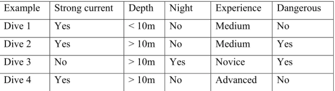
Table 1. Positive and negative training examples for the target concept

“Dangerous dive”...13 Table 2. Average precision on large test set. ...61 Table 3. The set of states for each sub-class...71 Table 4. Confusion Table...77 Table 5. Mean average precision for DT HMM and 2-D MHMM...87 Table 6. The number of states for each sub-class. ...95 Table 7. Number of ancestors for each direction...96 Table 8. Machine learning terminology...119 Table 9. Notation for classification algorithms...120 Table 10. Notation for HMMs. ...120 Table 11. List of abbreviations. ...121

xxx

LIST OF FIGURES

Figure 1. The human brain is a pattern recognizer...8 Figure 2. Architecture of a model-based control strategy...9 Figure 3. An example surface of a two-dimensional Gaussian mixture PDF with

three components. ...19 Figure 4. The Bayesian network (BN) spells out the factorization that is a

simplification of the chain rule of probability. ...21 Figure 5. The one-dimensional hidden Markov model...23 Figure 6. (a) Image decomposition into blocks, (b) states of the Markov model. ..28 Figure 7. First-order neighborhood system for MRF-based models...30 Figure 8. State dependency according to the second order Markov mesh...32 Figure 9. The observation for the word “ul” and the pseudo 2-D HMM...34 Figure 10. Subset of state configuration along diagonals. ...35 Figure 11. Viterbi state transition diagram. ...37 Figure 12. 2-D Neighbors. ...40 Figure 13. Example of a random dependency tree...41 Figure 14. The inside probabilities...42 Figure 15. The outside probabilities...45 Figure 16. Image Categorization Scheme. ...52 Figure 17. Images decomposed into blocks with different sizes; (a) 44x40, (b) 16x15 and (c) 8x8 pixels...52 Figure 18. DCT coefficients of a 8 x 8 image block. ...53 Figure 19. Images annotated “Waterscape_Waterfront” from the TRECVid 2005

xxxi

Figure 20. Likelihood of the training data for three different gpm’s ...54 Figure 21. 20 top ranked images are uni-colored...55 Figure 22. The first true positive appears on position 122 of 9473 test images...55 Figure 23. Avg. precision for block size: (1) 176x120, (2) 88x60, (3) 44x40, (4)

16x15, (5) 8x8, (6) 4x4, (7) 2x2 ...57 Figure 24. Codewords in three dimensional space. Input vectors are marked as a

cross and codewords as an arrow...59 Figure 25. Global LBG Histogram...60 Figure 26. Recall / Precision for Beach ...61 Figure 27. 20 top ranked images using a combination of the global model and

DT HMM. ...62 Figure 28. 20 top ranked images using the DT HMM. ...62 Figure 29. The Joint probability of the observation given the model, and the tree, at

position (i,j)...64 Figure 30. State alignment with two different trees. ...65 Figure 31. Convergence of probability average. ...66 Figure 32. Distribution of scores...67 Figure 33. Example of images with mixed class areas. ...71 Figure 34. Annotating an image segment as “sky”. ...72 Figure 35. Image segmentation schema. ...72 Figure 36. Example of training images. ...73 Figure 37. State segmentation after 0, 2, 6 and 10 iterations. ...74 Figure 38. Likelihood of the training data. ...74 Figure 39. State segmentation on test image...75 Figure 40. Better performance with smaller minimum variance for GMMs. ...75 Figure 41. Test images with ambiguous regions...76 Figure 42. Labeling without/with transition probabilities...76 Figure 43. Example of segmented images. ...77 Figure 44. Quad-tree view of the parent-child dependencies of the 2-D wavelet...80 Figure 45. Hierarchical Multiresolution Model. ...81 Figure 46. Linear combination of multiple resolution models...83 Figure 47. Multiresolution classification scheme. ...84

xxxii

Figure 48. Three resolutions with constant block size: (a) 4x3, (b) 16x12 and (c) 64x48 blocks...85 Figure 49. Examples of training images for “beach”. ...85 Figure 50. Total likelihood during training...86 Figure 51. Precision recall for 2D-MHMM and DT-MHMM. ...86 Figure 52. Top ranked images by the DT-MHMM...87 Figure 53. Random 3-D Dependency Tree. ...91 Figure 54. Training image and initial state configuration using annotated regions..95 Figure 55. Original video sequence; first frame in upper left corner, followed by

every second frame. ...97 Figure 56. Frame segmentation in the final labeling (a) frame 1, (b) frame 12, (c)

frame 24. ...97 Figure 57. Object tracking of two skiers...98 Figure 58. Frame segmentation using complementary dual trees, (a) frame 1, (b)

frame 12, (c) frame 24. ...99 Figure 59. Perspective view of object tracking using complementary dual trees. ....99 Figure 60. Object tracking with smoothing over 50 random trees...100 Figure 61. DCT coefficients of an 8 x 8 image block. ...110 Figure 62. Example of Gabor kernels at 4 scales and 8 orientations ...111 Figure 63. Example of marked edges in an image using Canny's algorithm. ...112 Figure 64. DT HMM object relations. ...116 Figure 65. Low-level feature extraction objects...117 Figure 66. DT HMM object relations. ...118

1

Chapter 1

Introduction

1.1

Motivation

The average person with a computer will soon have access to the world's collections of digital video and images. However, unlike text that can be alphabetized or num-bers that can be ordered, there is no general formalism to organize image and video. Although tools which can ``see'' and ``understand'' the content of imagery are still in their early years, they are now at the point where they can provide significant assis-tance to users in navigating through visual media.

The challenge in developing techniques for media semantics requires knowledge and techniques from a variety of disciplines and domains, many of them outside of traditional computer and information science. Image understanding is a kingpin thereof and is a most complex challenge of AI. To cover this complicated area of computer vision in detail it would be necessary to discuss many other branches such as; knowledge representation, semantic networks, image processing, classification algorithms learning from experience, etc. The central problem is to bridge "the semantic gap", which describes the difference between the meaning that users expect systems to associate with their queries, and low-level features that the systems actually compute. A number of researches have introduced systems that bridge the gap between low-level features and semantic classes [3], [5], [6], [8], [25], [38], [52], [68].

Semantics is meaningful only in context; it can not exist without a knowledge base to project its concept on [35]. In this work we employ a probabilistic framework, which means that the knowledge database, the meta-data of the image is stored numerically and we use a state-transition model (a hidden Markov model) for capturing the context and dynamics of images and video.

2

The hidden Markov models (HMM) have been successfully introduced to many important problems in image processing such as computer vision or pattern recogni-tion. Their success is due to both their rich mathematical structure which engenders a theoretical basis for many domains, and to the Baum-Welch algorithm [38]. The Baum-Welch procedure is an efficient training algorithm that allows estimating the numeric values of the model parameters from training data.

However for images computations becomes intractable because of the statistical dependencies in two dimensions. Many approaches have been proposed to preserve a modest computation [39], [44], [49], [50]. The disadvantages of these approaches is that they either greatly reduce the vertical dependencies between states, which is then only achieved through a single super-state, or introduces simplifying assumptions and approximations so that the probabilistic model is no longer theoretically sound.

1.2

Contribution and Outline

In this thesis we present a new type of multidimensional hidden Markov model that is efficient in computational complexity and storage, while still being theoretically sound. The basic idea is to relax the joint dependencies between neighboring states by a dependency tree.

We derive the necessary expressions for the procedures associated with HMMs such as the Baum-Welch and Viterbi algorithms. The model is embedded in an image modeling framework for benchmarking and investigating the properties of the formalism. The experimental parts deal mostly with classification problems since they are easy to evaluate and due to the fact that we have access to a common anno-tated video database used by the TRECVid workshop [66]. The outline of the dissertation is as follows:

• Chapter 2 provides a perspective of image understanding from outside of tra-ditional computer and information science. I review the literature on statistical learning methods and give an introduction to the discipline of Markov models.

• Chapter 3 constitutes the theoretical core of this dissertation. Here we present our new hidden Markov model based on a random dependency tree, which will later be referred to as the dependency tree hidden Markov model

(DT HMM). The algorithms associated with HMMs are derived and we show that for this model, most of the common algorithms keep the same linear complexity as in one dimension. We provide experimental details and com-pare the results with those of the TRECVid workshop.

• In chapter 4 we specialize the model to the problem of image segmentation. We review the current state-of-the-art and present a solution based on the

3

DT HMM. Semantic regions are implemented by restricting a number of states to a sub-class. This chapter also deals with the expansion to multiple resolutions. The extension allows an image to be represented by observations in several resolutions which corresponds to local and global context. Com-parisons, in an image classification scenario are made between the multiresolution DT HMM and another well known multiresolution model. • Chapter 5 considers an extension to three dimensions in a video modeling

scenario. Since video can be regarded as images indexed with time, we gen-erate a 3-D dependency tree and compute the transition probabilities over space and time. We demonstrate the potential of the model by applying it to the problem of tracking objects in a video sequence. We explore various is-sues about the effect of the random tree and smoothing techniques. Experiments demonstrate the potential of the model as a tool for tracking video objects with an efficient computational cost.

5

Chapter 2

Image Classification

A picture can be very useful in answering questions. Like how where people dressed during the 1860’s or how does a Lemur look like? However, retrieving a picture that answers a particular question can be difficult. Investigating the meaning of pictures can be compared to subject analysis of text, where the sense of the words are of concern not the words of the text, nor the bibliographic description or genre exempli-fied by the work.

In this chapter we present a survey of the literature on image classification. We start with a review outside computer science by touching different linguistic and cognitive aspects of image understanding. I look for answers to questions such as “what is the meaning of a picture?” and how can the relation between visual objects in an image be described? We then present important classification techniques in section 2.4.

2.1

Image Understanding

Image understanding is one of the most challenging fields of machine learning, and it depends on other independent domains such as: knowledge representation, semantic networks such as ontologies, inference, classification, segmentation, learning from experience and more.

Some successful attempts to model media semantics make use of ontologies1 [28], [29]. The advantage of ontology learning is that its influence path is based on

1 _{In this context an ontology denote a taxonomy with a set of inference rules.}

In philosophy, ontology (from the Greek ὄν, genitive ὄντος: of being (part. of εἶναι: to be) and -λογία:

6

ogy hierarchy, which has real semantic meanings. In ontology-based learning there are two kinds of influences; boosting and constraints. Boosting is about boosting the precision of concepts by taking the results from more reliable ancestors. The con-straints are used to decrease the probability of miss-classifying concepts that cannot coexist.

2.1.1 The Meaning of the Picture and Ontologies

To decide the subject of a picture, it is necessary to determine the meaning conveyed by the images within, and the relationship between this meaning and the words used to describe it. In analyzing the kinds of meaning a picture may have, and the relation-ship between the words used to describe it. Shatford [1] proposes a system for classifying the subjects of a picture, into Generic Of, Specific Of and About. First the

meaning can be divided into the generic description OF the represented objects and

actions, and the intrinsic meaning of the content (ABOUT). Since pictures are

simul-taneously generic and specific; a picture of a bridge is both that particular bridge and the generic bridge. She divides the Ofness into generic and specific, so we have:

Generic Of: Ofness, equivalent to the generic meaning of an image. Requires only “everyday familiarity with objects and actions” e.g. man, woman, child, lifting a hat. Skyscraper , Office Building.

Specific Of: Demands educational knowledge like “familiarity with specific themes and concepts”, e.g. to understand that haft-lifting is a Greeting gesture”, or a particu-lar building is the Chrysler Building. There can be several specific subjects in a picture (referents) that determine the sense of the picture (c.f. meronony below).

Generic About: Description of a mood, identification of mythical beings that have no concrete reality, or symbol meanings abstract concepts communicated by images. Emotions; love, sorrow and concepts: truth, honor and strength, e.g. expressional like “the pity of the Crucifixion”, “modern architecture”.

2.1.2 Hyponomic Ontology

The crux is to determine the meaning of a picture so that we can classify it in accor-dance with its meaning. Only then will the user be able to search content on whatever level: generic or specific. This is particular useful since a user can only express the needs in terms of what s/he knows. A hyponomic ontology (hyponomy = is-kind-of

relationships) will allow us to retrieve specific content by performing a generic search, i.e. the user can search on a subject without knowing its specific name. A side effect is that the user might learn specific facts. E.g. a search on “Gothic church” can retrieve Notre Dame. In this way one could say that we use an ontology to map between the specific- and the generic as mentioned above. We employ this kind of

7

ontology in the personalization engine for interactive TV [16], in order to match video object concepts with user preferences.

Introducing the relation ship of Aboutness, the description of a mood or a symbol,

would extend the possibilities to search for a picture that represents strength, vanity or modern architecture. It is perhaps worthwhile mentioning that the factual meaning is easier to classify as people are more likely to agree on descriptions on objects rather than an emotion or mood.

2.1.3 Meronomic Ontology

Some attempts have been made to weight co-occurring multimodal features in order to infer the occurrence of semantic objects [3]. In a model based approach [68], Golshani et Al. measured the semantic similarity of quantized visual cue’s using a correlation matrix and then mapped them to semantic labels. An ontology was integrated to further facilitate the translation of text queries into visual queries. Hence if there was no model learned for a certain key word the semantically closest will be subsumed from the ontology by finding the hyponyms. The underlying idea resem-bles that of LSI; to express a certain topic in text a certain collection of words will be used. The collection will be perturbed by the existence of synonyms and polysemous word.

Another approach would be to use a meronomy ontology (meronomy = part-whole relationship) to map co-occurrences of several referents to a subject. A picture is characterized by one or several objects (or referents in [1]). Shatford proposed a

method of thresholds recommendations; only name what is whole, not necessarily an integral part of a larger whole. In our framework it would translate to use the ontol-ogy to name only larger parts and use the “has-a” relation (like in part-based object detection for example [4]).

As discussed earlier, since a picture can have several referents with its senses we can use an ontology to explain what sense the co-occurrence of some referents (visual obejcts) have. A cityscape consists of sky, buildings, roads, rivers etc. On a lower

level of detail one might say that the presence of a large number of windows in rows formed in layers, with walls and a roof forms a skyscraper, similar to the “is-part-of “ relationship.

The need of co-occurrence and spatio-temporal information is even more important in presence of blur while performing object recognition. As pointed out by the authors in [6] the sense of an image is strongly judged by the position of the objects within an image and not their shape.

The structure of an ontology can also be used in order to choose an adequate feature model for each type of image, as well as different classifiers for different problems. In a system developed by Minka and Picard [2] it is assumed that there is no single model that can capture everything what humans perceive in images, their system used a “society of models”. The system internally generates several groupings of

8

each image’s regions based on different combinations of features, then learns which combinations best represents the semantic categories given as examples by the user.

2.1.4 Notes from Cognitive Psychology

According to the theory of cognitive science, the impressive abilities demonstrated by the human brain originate mainly from one basic ability: pattern recognition. Our brain is a generalized pattern-recognition machine. For example, there are many different shapes for tables, but somehow we always implicitly recognize a table when we see one, even if we have never seen that particular one.

In some particular cases, the human brain’s ability to recognize patterns is overeager, so that it recognizes patterns where there are none. This phenomenon is called pareidolia, and is sometimes used to explain phenomena’s like the Loch ness mon-ster, astrology and the man in the moon. The effect is easy to recall; try to count the black dots in the figure below.

Figure 1. The human brain is a pattern recognizer.

2.2

Knowledge Representation and Control Strategy

Pictures are a kind of sensory data, and there is a lot of work going on to figure out how to index this sensory data. What kind of knowledge representation should be used for its meta-data? Currently the most important attempts to provide standards for description of content are MPEG-7 from ISO, and the semantic web from the W3C. In a paper by Ramesh Jain [31] some interesting ideas are presented on how to store and interact with spatio-temporal data.

As I mentioned in the introduction, the computed feature-based signatures by them selves infer nothing about the content, only that the content is different from sur-rounding clusters. To extract meaningful semantics a knowledge base is needed to project concept on. The content and representation of this knowledge is of main concern.

9

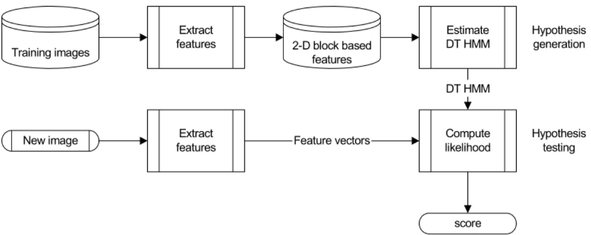
In this thesis we use a 2-D HMM as the backbone of the knowledge representation in conjunction with a set of sub-class definitions. The HMM is a generic model, that works in a top-down fashion which mean that an internal model is generated and is verified against a test collection Since a top-down model is only testing to retrieve images that we know something about, there is no limitation in adding prior knowl-edge limited to a certain domain. We can for instance add “is-part-of” knowlknowl-edge (c.f. section 2.1.3) such as sky, sea and sand are parts of the concept beach. An

example of this is illustrated in section 4.1.2.

The architecture of a generic top-down classification system is depicted in Figure 2. The principle of a top-down control is the construction of an internal model and its verification, meaning that the principle is goal oriented, like looking for your car at a

parking lot.

Training images

Extract

features 2-D block based

features Estimate DT HMM Compute likelihood Extract features

New image Feature vectors

DT HMM Hypothesis generation Hypothesis testing score

Figure 2. Architecture of a model-based control strategy.

The image understanding process consists of sequential hypothesis generation and testing. The hypothesis testing algorithms represent data by a set of points (or proto-types). A class is assigned to each prototype by majority vote on the associated class distribution of the prototype. A test feature vector is identified as the class of its closest prototype.

2.3

Applications

There are many areas of applications for image understanding: robot vision, remote sensing, surveillance applications, military applications, medical image understand-ing, and entertainment. In this section we shall present some examples from each category.

10 Robot Vision

Engineers at DaimlerChrysler are working on technology that can make cars watch out for hazards, listen to the driver or even know when he/she is distracted, in order to alert the human driver to potentially dangerous situations.

Prototype cars, equipped with stereo cameras are able to recognize hazards that the driver has overlooked – like some one running over the road or a bouncing ball. It is able to spot traffic lights and by swift camera movements is even able to check that they are still green when the car approaches [7].

Remote sensing

In remote sensing for forestry applications the main goal is to fully or partly replace the human image interpreter by a seeing computer, capable of making many deci-sions on its own, with a minimum of human intervention during the image processing and analysis. A review of the state-of-the-art of the research from different countries is given in Hill and Leckie [8].

Unsupervised extraction of roads eliminates the need for human operators to perform the time consuming and expensive process of mapping roads from satellite imagery. As increasing volumes of imagery become available, fully automatic methods are required to interpret the visible features such as roads, railroads, drainage, and other meaningful curvilinear structures in multi-spectral satellite imagery. The challenge of detecting curvilinear elements is also related to the problem of deriving anatomical structures in medical imaging as well as locating material defects in product quality control systems and cartographic applications [9].

Surveillance Applications

Surveillance applications often collect a large amount of video data. Currently the surveillance applications do not allow the user to quickly search the collected data for an occurrence of a particular individual. Face based browsing for surveillance applications such as ID system for the police force to detect the face of criminals, may enhance airport security.

The ultimate goal of surveillance systems is automatic detection of events and suspicious activities that triggers an alarm (detection) as well as reducing the volume of data presented to human operator (retrieval). Event detection requires interpreta-tion of the "semantically meaningful object acinterpreta-tions". Highway monitoring, airport surveillance, building access control are just a few of the several important applica-tions.

Whereas most models for detecting unusual events assume that “all” unusual event events can be modeled, which requires off-line training. The research lab MERL2 employs an unsupervised learning method that does not require definition of what is usual and what is not. They define usual as the high recurrence of events that are

11

similar. As a result, unusual is the group of events that are not similar to the rest, which also allows detecting multiple unusual events [10].

The same lab has also developed a technology for automatically detecting pedestrians in video sequences. Detecting and tracking pedestrians can be used to sound an alarm if an intruder is in a restricted area or to aid in browsing hours of surveillance video by skipping to the next part of the video where a person was seen.

The problem of detecting people in low resolution surveillance video is difficult because the pedestrian may be very small in the image, making the amount of information contained in the pixels small. Furthermore, there may be background movement in the scene such as trees waving or a cloud shadow passing by which makes causes motion detectors to fail. Their approach is to encompass both the appearance and the motion of pedestrians in the model [11].

Military applications

The future battlefield is characterized by an expanding suite of sensors and sensing modalities collecting vast volumes of imagery from a mixture of ground, air, and space-borne platforms. Image understanding techniques are needed to extract the information needed by military forces from this data-rich environment.

Image understanding in military applications also provide advanced vision systems to aid intelligence image analysts, or enables an unmanned military ground vehicle to scout for enemy targets [12], [13].

Medical Image Understanding

Clinicians routinely employ a variety of imaging techniques during patient diagnosis. The volume of information, and the difficulty of interpreting it, make this area one in which advanced image understanding can make significant improvements in the detection and treatment of illness e.g. 2-D functional analysis of the heart, mammog-raphy image analysis, identify lung cancer cells and discriminate among different lung cancer types [14], [15].

Interactive Television Projects

Advanced Digital Television provides an exciting new realm for the consumer. Not only does it offer improved picture quality, it also provides a means for seamlessly blending many new services into the TV set, expanding the scope of what televisions can do. Advanced Digital Television also poses new challenges in video encoding, transmission, and reception.

MPEG2 has been successfully adopted in digital broadcasting and computer video applications. Now the coding technologies are evolving from MPEG2 to MPEG4 which standardizes algorithms and tools for flexible representation of audio-visual data in an object-oriented manner.

The object-based compression in MPEG4 enhances the user's interaction with a device or computer. This aspect has been investigated in the GMF4iTV [16] project

12

and a demo version of the interactive video system were presented at 4th Workshop on Personalization in Future TV [17]. The objective of the prototype was to build an

end-to-end broadcast system for providing personalization and interactivity to TV programs through active video objects [18].

Entertainment

Vision-based interfaces for computer games allow the player to move or gesture to affect the game, instead of pressing buttons. The characters in the game may imitate those motions, or respond accordingly.

Vision can be a powerful interface device for computers. There is the potential to sense body position, head orientation, direction of gaze, pointing commands, and gestures. Such free and untroubled interaction can make computers easier to use. The application of vision to computer games poses special challenges. The response time must be very fast, while the total hardware cost must be very low. An approach in using fast and simple algorithms to meet these challenges is presented in [19].

2.4

Statistical Learning

Statistical modeling methods are paramount in today's large-scale image analysis. It is critical for almost all image processing problems, such as estimation, compression and classification. This section gives a brief introduction to the theory of inductive learning, followed by a presentation of the currently most important classification algorithms.

2.4.1 Concept Learning

In the process of learning, general concepts are formulated from specific examples. Humans incrementally learn new concepts such as “butterfly”, “prime numbers”, “explosion” etc. Each such concept can be viewed as describing some subset of objects or events over a larger set (e.g. the subset of insects that constitute butter-flies). A concept can be modeled as a function defined over this larger set, e.g. a function defined over all insects whose value is true for butterflies and false for all other insects.

In machine learning the desire is to induce3 a general function (a hypothesis) that best fit a set of training examples. This is sometimes referred to concept learning: the

problem of automatically inferring the general model of some concept, given exam-ples labeled as members or nonmembers of the concept.

3 _{Induction: the process of deriving general principles from particular facts or}