An elasto-plastic self-consistent model for damaged polycrystalline materials: Theoretical formulation and numerical implementation

Science Arts & Métiers (SAM)

is an open access repository that collects the work of Arts et Métiers Institute of Technology researchers and makes it freely available over the web where possible.

This is an author-deposited version published in: https://sam.ensam.eu Handle ID: .http://hdl.handle.net/10985/19156

To cite this version :

J. PAUX, Mohamed BEN BETTAIEB, H. BADREDDINE, Farid ABED-MERAIM, C. LABERGERE, K. SAANOUNI - An elasto-plastic self-consistent model for damaged polycrystalline materials: Theoretical formulation and numerical implementation - Computer Methods in Applied Mechanics and Engineering - Vol. 368, p.113138 - 2020

Any correspondence concerning this service should be sent to the repository Administrator : archiveouverte@ensam.eu

-1-

An elasto-plastic self-consistent model for damaged

polycrystalline materials: Theoretical formulation and numerical

implementation

J. Paux1,2,3_{, M. Ben Bettaieb}1,_{, H. Badreddine}3_{, F. Abed-Meraim}1_{, C. Labergere}3_{, K. Saanouni}3 1_{Arts et Metiers Institute of Technology, CNRS, Université de Lorraine, LEM3, F-57000, Metz,}

France

2_{IRT M2P, 4 rue Augustin Fresnel, F-57070 Metz, France}

3_{ICD/LASMIS, University of Technology of Troyes, UMR 6281, CNRS, Troyes, France}

Abstract

Elasto-plastic multiscale approaches are known to be suitable to model the mechanical behavior of metallic materials during forming processes. These approaches are classically adopted to explicitly link relevant microstructural effects to the macroscopic behavior. This paper presents a finite strain elasto-plastic self-consistent model for damaged polycrystalline aggregates and its implementation into ABAQUS/Standard finite element (FE) code. Material degradation is modeled by the introduction of a scalar damage variable at each crystallographic slip system for each individual grain. The single crystal plastic flow is described by both the classical and a regularized version of the Schmid criterion. To integrate the single crystal constitutive equations, two new numerical algorithms are developed (one for each plastic flow rule). Then, the proposed single crystal modeling is embedded into the self-consistent scheme to predict the mechanical behavior of elasto-plastic polycrystalline aggregates in the finite strain range. This strategy is implemented into ABAQUS/Standard FE code through a user-defined material (UMAT) subroutine. Special attention is paid to the satisfaction of the incremental objectivity and the efficiency of the convergence of the global resolution scheme, related to the computation of the consistent tangent modulus. The capability of the new constitutive modeling to capture the interaction between the damage evolution and the microstructural properties is highlighted through several simulations at both single crystal and polycrystalline scales. It appears from the numerical tests that the use of the classical Schmid criterion leads to a poor numerical convergence of the self-consistent scheme (due to the abrupt changes in the activity of the slip systems), which sometimes causes the computations to be prematurely stopped. By contrast, the use of the regularized version of the Schmid law allows a better convergence of the self-consistent approach, but induces an important increase in the computation

-2-

time devoted to the integration of the single crystal constitutive equations (because of the high value of the power-law exponent used to regularize the Schmid yield function). To avoid these difficulties, a numerical strategy is built to combine the benefits of the two approaches: the classical Schmid criterion is used to integrate the single crystal constitutive equations, while its regularized version is used to compute the microscopic tangent modulus required for solving the self-consistent equations. The robustness and the accuracy of this novel numerical strategy are particularly analyzed through several numerical simulations (prediction of the mechanical behavior of polycrystalline aggregates and simulation of a circular cup-drawing forming process).

Keywords:

elasto-plasticity, finite strain, Schmid criterion, damaged single crystal, polycrystal, self-consistent scheme, numerical implementation, metal forming.

1. Introduction

In the field of material engineering, the modeling of the mechanical behavior in the finite strain range remains an active research topic. It is of prime importance in the optimization of forming process parameters and in the prediction of formability limits of metallic parts and components. Indeed, most forming processes, such as rolling or deep drawing, induce large plastic deformations, which lead to significant evolution of the material properties (hardening, plastic anisotropy, damage…). It is well known that crystallographic slip accommodates most of the plastic strains, while inducing plastic anisotropy in the mechanical response by evolution of crystallographic texture and dislocation structures. Additionally, the development of transgranular and intergranular mechanical fields plays a significant role in the deformation process, especially during unloading and reloading states [1]–[7]. Furthermore, nucleation, growth and coalescence of micro-voids and micro-cracks lead to the limitation of the formability of metallic components [8]–[9]. Hence, the evolution of macroscopic mechanical fields is governed by the evolution of the microstructural properties. These microstructural properties cannot be accurately modeled by the classical phenomenological approaches. To overcome this limitation and thus to accurately capture these properties, several multiscale schemes have been proposed. The aim of the present paper is to detail the numerical implementation of a new multiscale scheme involving damage at the grain scale. The current model ensures both the accuracy of the physical description and the robustness of the numerical computation. In this innovative model, three physical scales are taken into account: the single crystal scale, the polycrystal scale and the structural scale.

 The single crystal scale: in this contribution, a new single crystal constitutive model is developed. This model follows a finite strain rate-independent formulation, which is more suitable to model the evolution of the mechanical behavior during cold forming processes [10]–[13]. In this model, plastic strain is mainly due to the slip along the crystallographic slip systems (CSSs) and the plastic flow rule is modeled based on the classical Schmid criterion [14] and on one of its regularized versions [15]. This model allows taking into account the damage effects on the plastic

-3-

behavior using the concept of continuum damage mechanics (CDM), where a scalar damage variable is introduced at each CSS [16]

–

[17].

The numerical algorithms used to integrate the rate-independent single crystal constitutive equations based on the classical Schmid criterion (CSC) can be categorized in two main families: the return-mapping algorithms [18]–[21] and the ultimate algorithms [22]–[26]. Akpama et al. [27] have conducted an extensive comparative study on these two families of algorithms. It appears from this study that the class of ultimate algorithms is largely more efficient and more robust than the return-mapping algorithms. Consequently, the ultimate algorithm has been extended in the current work to integrate the damaged single crystal constitutive equations based on the classical Schmid criterion (called hereafter for brevity DCSC). The main tedious task in the numerical integration of these equations concerns the determination of the set of active CSSs and the corresponding slip rates. To achieve this task, the consistency condition, expressed based on the DCSC, could be mathematically formulated as a Non-Linear Complementarity Problem (NLCP). When damage is not considered, several numerical schemes have been developed to solve this complementarity problem. In this particular case, Ben Bettaieb et al. [26] have developed an implicit integration scheme to accurately solve the NLCP. More recently, Akpama et al. [27] have developed an explicit algorithm to solve the same problem after its linearization allowing the transformation of the NLCP into a linear complementarity problem (LCP). The robustness and the efficiency of this explicit algorithm, compared to the implicit one, for the integration of undamaged single crystal constitutive equations have been highlighted in [27]. In the present contribution, damage evolution is introduced in the constitutive equations, which requires some special care to be taken in the numerical integration of the constitutive equations. In fact, to consider the damage evolution, we have extended the explicit algorithm developed in [27]. In this case, the LCP is transformed into a quadratic complementarity problem (QCP), which is solved by the combinatorial search scheme [18], for the identification of the set of active CSSs, and by the fixed-point algorithm for the computation of the corresponding slip rates.

When the regularized Schmid criterion (RSC) is used for the modeling of the plastic flow, the problem of the determination of the set of active CSSs is obviously avoided and all the CSSs are simultaneously activated (in the elasto-plastic stage). In this case, the constitutive relations defining the expression of the slip rates are quite similar to those used in a viscoplastic formulation [28]. For viscoplastic single crystals, it is well known that the high value of the regularization exponent parameter leads to a very stiff non-linear problem. In such a situation, the computation of the slip rates experiences some convergence difficulties [29]. Several numerical techniques have been developed in the literature to circumvent these difficulties, such as the k-modification method proposed in [29]–[30] and the spectral database crystal plasticity approach developed in [31]–[33]. In the current investigation, the regularized Schmid criterion is extended to take into account the damage over the CSSs. The resulting model (denoted DRSC in what follows) is

-4-

integrated by developing a semi-implicit integration scheme based on the Newton–Raphson method. The developed scheme combines both accuracy and efficiency of the numerical integration.

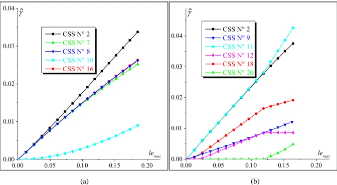
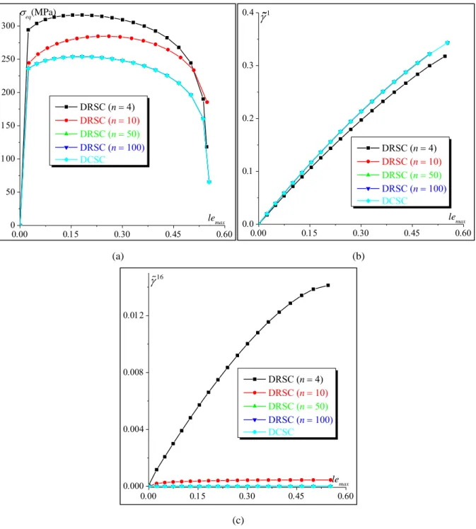
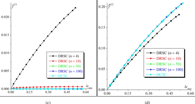
To compare the predictions based on the two single crystal models (namely the DCSC and DRSC), several numerical simulations are presented in this paper. From these predictions, it turns out that the results obtained by the DRSC coincide with those obtained by DCSC when the regularization exponent parameter is sufficiently high (typically higher than 100). However, the computation time required to integrate the constitutive equations based on the DRSC is largely higher than that required by the DCSC.

 The polycrystal scale: the self-consistent approach is used in the current contribution to achieve the transition between the single crystal and polycrystal scales. Compared to the full-field multiscale approaches, such as the FE homogenization technique [34] or the FFT approach [35], the self-consistent scheme (mean-field approach) seems to be a good tradeoff to describe, accurately and efficiently, the mechanical behavior of polycrystalline materials. The higher performance of the self-consistent scheme in terms of computation time is even more evident when these approaches are embedded into a finite element strategy to simulate forming processes. In addition, the self-consistent approaches enable to overcome the limitations of the mean-field Taylor model. In fact, the application of the self-consistent scheme allows taking into account the equilibrium conditions in order to approach the strain localization at the grain level. Then, it allows more accurately describing the influence and the evolution of the texture morphology and the interaction between the grains and their surrounding ones. Numerically speaking, solving the self-consistent equations consists in the iterative computation of the macroscopic tangent modulus, which is based on the microscopic tangent moduli that relate the microscopic stress rate to its conjugate strain rate. Within the small strain framework, all of the strain and stress measures coincide, and there is no doubt on the choice of the conjugate mechanical variables. However, under finite strain conditions, there are various conjugate strain/stress measures, and choices are based on dissipation analysis. In the framework of Euler formulation, several authors have selected the Jaumann derivative of the Cauchy stress tensor and the Eulerian strain rate (the symmetric part of the velocity gradient) as conjugate variables to formulate the self-consistent equations [36]–[40]. This choice allows simplifying the numerical implementation of the self-consistent approach, which ensures easier convergence conditions for the iterative computations, but leads to some theoretical inconsistencies. Hill [41] suggested the use of the velocity gradient and the nominal stress rate in order to establish the transition relationship between microscopic and macroscopic stress and strain measures. Based on this choice, Lipinski and Berveiller [42] and Lipinski et al. [43] proposed a self-consistent approach to polycrystal plasticity at finite strains. Thanks to its sound theoretical basis, this formulation is adopted in the present work. This choice may also lead to some convergence difficulties when the DCSC is used. These difficulties

-5-

are mainly due to the continuous change in the set of active CSSs during loading. This problem has been early pointed out in [44]. This issue is naturally avoided when the Schmid criterion is regularized, as all CSSs are simultaneously activated in the plastic loading phase. Consequently, to ensure the efficiency and the convergence of the self-consistent scheme, the DCSC is adopted to integrate the microscopic constitutive equations, while the tangent modulus determined by the DRSC is used to achieve the self-consistent transition. This strategy, very similar to the numerical solution adopted in [44], allows combining the benefits of the two approaches. To carefully investigate the effect of the Schmid criterion regularization on the computation time and on the mechanical response of polycrystalline aggregates, several numerical predictions are carried out. These predictions reveal that the use of the mixed DCRSC (i.e., DCSC for the microscopic model and DRSC for the self-consistent computations) self-consistent approach allows us to obtain the same results as those given by the self-consistent scheme based on the DRSC, but with significantly reduced computation efforts.



The structural scale:

the different versions of the self-consistent approach (with the different combinations of plastic flow rules and numerical techniques) have been implemented as a user-defined material (UMAT) subroutine into ABAQUS/Standard FE code. In the present implementation, special attention is paid to the handling of the material rotation at the different scales and to the satisfaction of the incremental objectivity. The efficiency of the present constitutive modeling is assessed based on several numerical simulations.

This paper contains three main sections:

 The first one is devoted to the theoretical aspects of the developed

constitutive

model. The self-consistent equations are recalled. Then, the single crystal constitutive equations are presented with special focus on their coupling with ductile damage.

 The second part deals with the numerical and algorithmic aspects related to the model implementation at different scales. The specificities associated with the ABAQUS/Standard UMAT are also described.

 The third section is dedicated to numerical applications and presentation of the simulation results. First, basic tests on a single FE are presented to highlight the interaction between the various mechanical phenomena modeled. Then, structural computations are presented to assess the robustness of the implementation and the prediction capabilities of the model.

Conventions, notations and abbreviations

The following conventions and notations are adopted throughout this paper. Note that the assorted notations can be combined, while additional notations will be clarified as needed in the text:

-6-

 Vectors and tensors are indicated by bold letters or symbols. However, scalar parameters and variables are designated by thin and italic letters or symbols.

 Einstein’s summation convention of implied summation over repeated indices is adopted. The range of free (resp. dummy) index is given before (resp. after) the corresponding equation.   time derivative of .

  the effective counterpart of the variable  (in the framework of damage mechanics).  T _{transpose of} _.

 C _{corotational derivative of} _.

 1 _{inverse of} _.   absolute value of .

  positive part of  or McCauley brackets.  e _{exponential of .}

  . simple contraction or contraction on one index (inner product).   : double contraction or contraction on two indices (inner product).   tensorial product (external product).

 CSS crystallographic slip system.

 CSC model based on the classical Schmid criterion and the associated algorithm.  RSC model based on the regularized Schmid criterion and the associated algorithm.  DCSC model based on the damaged classical Schmid criterion and the associated algorithm.  DRSC model based on the damaged regularized Schmid criterion and the associated

algorithm.

2. Constitutive framework

2.1. Polycrystal modeling

The mean-field self-consistent approach developed by Lipinski et al. [42]–[43] is used to model the mechanical behavior of polycrystalline aggregates starting from the behavior of their constituent grains (or crystal). In the self-consistent approach, each grain is assumed to be an ellipsoidal inclusion surrounded by a fictitious homogeneous and infinite medium that has the same properties as the polycrystal. As stated by Hill [41], within the framework of finite strains, the macroscopic Eulerian velocity gradient G and the macroscopic nominal stress rate N should be selected as suitable strain

-7-

and stress measures to build the multiscale scheme. These macroscopic tensors are related to their microscopic counterparts g and n by the Hill averaging theorem:

 

 

1 1 d ; d , G



g x N



n x V V V V V V (1)

where x is the vector of coordinates of a material point in the polycrystalline aggregate of volume V . The macroscopic nominal stress tensor N is related to the macroscopic Cauchy stress tensor Σ by the following relationship:

1

,

Σ

NJ F  (2)

with F the macroscopic deformation gradient and J its determinant.

By inversion of Eq. (1), the microscopic velocity gradient and nominal stress rate are linked to their macroscopic counterparts by the following relations:

 

 

: ;

 

 

: ,

g x A x G n x B x N (3)

where A x

 

and B x

 

are fourth-rank concentration tensors for the velocity gradient and the nominal stress rate, respectively.

The self-consistent approach allows linking N to G through the macroscopic fourth-rank tangent modulus :

: .

N G (4)

At the microscopic level, a relationship similar to Eq. (4) can be derived by combining the constitutive relations of the single crystal:

     

: ,

n x  x g x (5)

where is the microscopic fourth-rank tangent modulus. The relation between and can be obtained by combining Eqs. (4)–(5):

   

1 : d . x A x 

_

V V V (6)

Furthermore, it is assumed that all mechanical variables are homogeneous within each individual single crystal. Thus, for any grain gr , Eqs. (3)1and (5) become:

: ; : .

ggr Agr G ngr gr g gr (7)

By using Green’s tensor and some classical mathematical developments [45], an approximate version of the concentration tensor Agr is given by the following expression:









1









1 1 4 4 1 : : : , A I T I T          _   _ 



 Ngr gr gr gr gr gr gr gr f (8)

-8-

where I is the fourth-rank identity tensor, ₄ Tgr is a fourth-rank tensor describing the interaction

between grain gr and its surrounding ones, and

N

gr is the total number of grains within the polycrystalline aggregate. Tensor Tgr is mainly dependent on and its explicit analytical expression can only be found for isotropic elastic solids. For the proposed finite strain model, which involves strong textural and morphological anisotropy induced by the plastic strain and lattice spin, the interaction tensor Tgr _{is computed based on Fourier’s transforms [45]–[46] through an integral over an ellipsoid}

representing the grain gr . The macroscopic tangent modulus derived by the 1-site self-consistent version of the incremental scheme of Hill [41] is finally obtained as follows:

1 :A ,  



Ngr gr gr gr gr f (9)

where _fgr _{is the volume fraction of the grains having the same crystallographic orientation.}

2.2. Single crystal modeling

The single crystal constitutive modeling can be classically expressed in the form of Eq. (7). To reach this form, the single crystal kinematics are briefly revisited in Section 2.2.1. Then, the elastic part of mechanical behavior is formulated in Section 2.2.2. After that, the rules used to model the single crystal plastic flow are detailed in Section 2.2.3. Finally, the analytical expression of the microscopic tangent modulus is derived in Section 2.2.4.

2.2.1. Single crystal kinematics

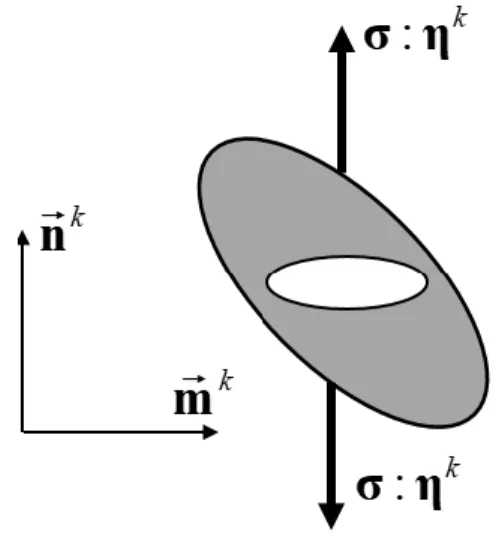
The kinematics equations of finite strain crystal plasticity, leading to the additive decomposition of the microscopic velocity gradient g into elastic and plastic parts, are provided in Appendix A. These kinematics equations are required to clearly present the single crystal constitutive framework based on the assumption that the plastic strain is uniquely due to the slip on N CSSs. Each CSS _s k is defined, in the deformed configuration, by two vectors mk and nk standing for the slip direction and the normal to the slip plane, respectively (Fig. A.1). The symmetric and skew-symmetric parts of the tensor product mk nk (which is known as the Schmid orientation tensor for CSS k) are denoted by μk and sk, respectively. In the intermediate configuration related to the crystallographic lattice defined by rotation

re _{(Fig. A.1), the counterparts of m}k

and nk remain fixed throughout the deformation. In most single crystal models, it has been assumed that the contribution of CSS k to the single crystal plastic deformation is coaxial to the Schmid tensor μk. But sometimes, this coaxiality property is not fulfilled, as crystallographic slip on this system may induce other phenomena, such as crack propagation leading to plastic deformation not coaxial to μk [16]. To take into account this effect, a second-rank tensor μk is introduced, which describes the deviation of the plastic strain from the Schmid tensor. The explicit

-9-

expression of tensor μk, along with further developments, will be given in Section 2.3. As a result, tensors dp _{and w}p _{can be expressed as:}



+



; 1,..., , p k k k s p k k γ k N γ  _  _    d μ μ w s (10)

where the plastic spin _wp _{characterizes the evolution of the difference between the rotation rate} r

r w of the current configuration and the rotation rate re were

of the single crystal lattice (the intermediate configuration) with respect to the initial configuration. The different configurations (namely, initial, intermediate and current configurations) are schematically illustrated in Fig. A.1. For practical reasons, and for handling only positive values of slip rates in the subsequent theoretical and numerical developments, it is more convenient to split each CSS into two opposite oriented CSSs



m nk, k



_and





,

m n

 k k _{, numbered}

k and k + N , respectively. With this decomposition, Eq. _s (10) is transformed into the following form [27]:



+



with 0 ; 1,..., 2

.

d μ μ w s  _  _{ }    p k k k k s p k k γ γ k N γ (11)

2.2.2. Single crystal elastic model

The effect of damage evolution on the single crystal behavior is thoroughly considered in the current model. Damage is assumed to affect both elastic and plastic properties. To satisfy the objectivity principle, the lattice corotational derivatives σc of the Cauchy stress tensor σ is related to the elastic strain rate by the following damaged hypoelastic model [17]:

. . : : ,

σc σ w σ σ w e  e c de ec εe e

(12) where εe is the integral of the elastic strain rate de over the loading history in the lattice corotational frame, and ce is the elasticity modulus for the damaged materiel, which is related to its counterpart for undamaged materiel ce by the following classical relation [47]:



1



.

ce  d_av ce (13)

The scalar damage variable d_av describes the effect of micro-damage on the elastic properties and its evolution equation will be given later in Eq. (28). In the present work, the elasticity of the undamaged material is assumed to be infinitesimal, linear and isotropic. Hence, matrix ce _{only depends on the}

Young modulus E and the Poisson ratio  .

2.2.3. Single crystal plastic flow rules

Two versions of the Schmid flow rule have been extended to take into account the effect of damage on the single crystal plastic behavior: the classical Schmid rule and the regularized version developed by

-10-

Gambin and Barlat [15]. For the sake of brevity, the formulated extended flow rules will be called in what follows DCSC (damaged classical Schmid criterion) and DRSC (damaged regularized Schmid criterion).

2.2.3.1. DCSC

To define the damaged classical Schmid criterion, let us introduce the resolved shear stress, which is defined as the projection of the Cauchy stress tensor σ on the Schmid tensor of CSS k:

1,..., 2 σ μ: ,

   k  k

s

k N τ (14)

and the critical shear stress τ_ck defining the limit of the single crystal yield locus. The evolution of τ_ck is described by the following generic hardening rule:

1,..., 2 ; 1,..., 2 ,

   k  kl l 

s c s

k N τ h γ l N (15)

where h is an interaction hardening matrix. The components of this matrix are generally variable and depend on the accumulated slip on the different CSSs.

To consider the ductile damage effect on the plastic behavior, a damage variable dk is introduced for each CSS. Thus, the ‘actual’ resolved shear stress _{τ and slip rate} k _{γ are linked to their effective} k

counterparts τ and k γk by the following relations, based on the energy equivalence assumption [16]:

1,..., 2 ; 1 . 1        k k k k k s _k τ k N τ γ d γ d (16)

By using the effective variables, the classical Schmid criterion can be extended to take into account the effect of damage evolution on the plastic flow [16]:

2 1,..., 2 0 ; 0 ; 0 ,     k  k  k



Ns r k  k k k  s η c r k N f τ α σ d τ γ γ f (17)

where fk is the effective yield function corresponding to CSS k, α is a material parameter related to the damage-induced softening phenomenon, and k

η

σ is an effective crack-opening stress, normal to the

slip plane k, defined by the following relations:

1,..., 2 and : . 1 σ η       k η k k k s η _k η σ k N σ σ d (18)

In Eq. (18), ηk is a second-rank tensor corresponding to the opening of the micro-cracks in the slip plane nk, which is defined as follows:

1,..., 2 η n n η η ,

   k  k  k  k  k

s h dev

-11-

where ηk_h (resp. ηk_dev) is the hydrostatic (resp. deviatoric) part of tensor ηk_{. Equation (18) states that the}

slip system resistance weakens when σ η: k 0, which corresponds to micro-crack opening, while this resistance remains unchanged when σ η: k 0

. A schematic illustration of the physical influence of tensor ηk is depicted in Fig. 1. As will be shown hereafter, the presence of the hydrostatic component

ηk

h induces plastic compressibility [48].

Fig. 1. Schematic illustration of the influence of microcracks opening on the resistance of a typical slip system.

As for the case of the classical model, the yield locus corresponding to the damaged classical Schmid criterion (DCSC) given by Eq. (17) is a non-smooth surface, which is defined by the intersection of multiple planes (see Fig. 2).

It is worth noting that, without micro-cracks (i.e., when _dk 0 _{for all CSSs), the crack-opening stress}

k η

σ does not enter the expression of the flow rule (see Eq. (17)) and, hence, has no influence on it. However, when damage is considered in the modeling, k

η

σ induces some dependence of the plastic flow

on the hydrostatic stress, which is known to affect the metal failure. For simplicity of the upcoming developments, let us introduce the slip variables _{τ and} k k

c  defined as: 2 2 _{0 if 0} 1,..., 2 ; with . 1 otherwise η             _{ } 



Ns



Ns k η k k k r k k k k r k s η c r r σ k N τ τ α σ d   α s d s (20)

Considering the above definition of τ and k k_c, the effective yield function fk can be rewritten as: : 1,..., 2 . 1 σ         k k k k c k s c _k c k N f τ τ τ d  (21)

-12-

In the meanwhile, the plastic deformation induces propagation of micro-cracks, and thus a normal deformation component, due to the surface tension of the micro-cracks. Considering this phenomenon, a normal strain term is added to the plastic strain:

2 ( + ) ; 1,..., 2 . d μ η  



Ns  p k k k r s r γ α d k N (22)

By comparing Eqs. (11)1 and (22), the expression of tensor μk can be identified:

2 1,..., 2 : μ η .    k  k



Ns r s r k N α d (23)

As for the yield function fk, one defines the equivalent Schmid tensor corresponding to the plastic strain as: 2 1,..., 2 _d η     p  



s N k k k r s r k N   α d . (24)

The insertion of Eq. (24) into Eq. (22) allows us to give the following expression to dp:

; 1,..., 2 1

.

d d    p k p k s k γ k N d  (25)

Hence, plastic strain has a hydrostatic component leading to an induced volume variation, or compressibility induced by the term controlled by the micro-crack opening (see Eq. (19)). Moreover, the plastic behavior is no longer associative. Indeed, plastic associativity would have implied that:

; 1,..., 2 , 1 d σ      _ k k p k k c s k f γ γ k N d  (26)

which is not always verified, as

dp 

k k

c

  when σηk 0 (which corresponds to a tension state). A relevant thermodynamically-consistent formulation has been established by Saanouni et al. [17] to ensure the physical consistency of this plasticity flow rule. In practice, this non-associativity induces a difference between tension and compression states, which is consistent with crack-propagation framework. The above equations are complemented by the evolution equation of the ductile damage variable _{d . In} k

the current contribution, the model developed by Saanouni et al. [17] is adopted:





0





1 1,..., : . (1 )         _{ }      s s s k k+N k+N k+N k k k k s k m β Y Y k N d d γ γ γ γ υ S d (27)

This evolution equation depends on the thermodynamic force Y , associated with the damage variable k

k

-13-

The evolution equation of the averaged damage variable d , introduced in Eq. _av (13), is related to the rate of the slip damage variables _dk _by:

2 1 . 2  



Ns k av k s d d N (28) Since 1,..., : ,   k  k+Ns s k N υ υ (29)

equation (28) can be reformulated as:









2 2 2 1 1 1 1 1 1 1 . 2 2            _    _  



s



s



s



s s s s N N N N k N k N k k k k k k k av k k k N k s s s d d γ γ υ γ γ υ γ υ N N N (30) 2.2.3.2. DRSC

A regularized form of the Schmid criterion (RSC) has been developed by Gambin and Barlat [15]. Contrary to the CSC defined by a non-smooth yield locus, the regularization of the Schmid criterion allows smoothing the corresponding yield function (see Fig. 2). The RSC is extended in the current investigation to integrate the damage effects. The yield function corresponding to this regularized version reads: 2 1 1 0 , s n N k reg k k c τ f τ     _{ }    



(31)

where n is a positive integer acting as a regularization parameter. When parameter n goes to infinity, the regularized yield function given by Eq. (31) tends to the classical yield function, as illustrated in Fig. 2.               __ RSC (n10) RSC (n 50) RSC (n 100) CSC __         _  RSC (n 10) RSC (n 50) RSC (n100) CSC __

-14-

(a) (b)

Fig. 2. Effect of the regularization parameter n on the shape of FCC single crystal yield locus: (a) Complete yield loci; (b) zoom on the corner zone.

In the same spirit as the DCSC, the plastic strain rate dp derived from the DRSC can be defined as follows: 2 1 1 , 1 d d       _{ }   



s p n _k N k p k _{k k} k c _c τ λ n τ _{d τ}  (32)

where λ is the plastic multiplier.

It must be noted that, as for the DCSC, the normality rule is not fulfilled here as: 2 1 1 2 . 1 d σ        _{ } 



_{  } s n k N k reg p c k _{k k} k c _c f τ λ λ n τ _{d τ}  (33)

The flow rule for the DRSC can be defined by the following two inequalities and equality (equivalent to Eq. (20) for the DCSC):

0 0.

   _reg  _reg 

λ f λ f (34)

The expression of the slip rates for the different CSSs can be identified from Eq. (32):

2 1 2 1 2 2 1,..., : : ; : ,            _{ }    _{ }      s s n n k k k N k N k k s k k k k c c c c n τ n τ k N γ λ λ γ λ λ τ τ  τ τ  (35)

where k is a slip variable defined to simplify the subsequent developments.

2.2.4. Computation of the single crystal tangent modulus

A general expression for the microscopic tangent modulus , valid for both DCSC and DRSC, is derived in the current section. As stated by Eq. (7),this tangent modulus allows us to relate the nominal stress rate n to the velocity gradient

g

. The microscopic nominal stress n is related to the microscopic Cauchy stress σ by the microscopic counterpart of Eq. (2):

1

j  

 

n f σ (36)

Time derivation of equation (36) allows obtaining, after some mathematical developments detailed in [42], the following expression for the nominal stress rate n :

 





1 . . , j  tr    n f σ g σ g σ (37)

where j is the determinant of the microscopic deformation gradient f . By adopting an updated

-15-

 

1

. : ,

n σ tr g σ g σ σ   g (38)

where the fourth-rank tensor 1 _{is given by the following index form:}

1   _.

ijkl δ σkl ij δ σki lj (39)

The expression of the Cauchy stress rate σ, required in Eq. (38) to compute n , is obtained by combining Eqs. (A.7) and (12):













2 : : . . : : : : . . , σ c d d c ε w w σ σ w w g c d c ε c d σ w w σ              e p e e p p e e e e p p p (40)

where 2 is a fourth-rank tensor defined by the following index form:





2 1 . 2     ijkl δ σki lj δ σil kj δ σlj ik δ σjk il (41)

On the other hand, ce _{can be determined by combining Eqs. (13) and (30):}

1 ; 2 . ce   _avce   l lce  _s s d γ υ l N N (42)

By using expression (42) for ce and Eqs. (11)2 and (22) defining wp and dp, one can deduce the following expression of σ: 2 2 1 : . . 1 : : : , 1 d c σ s s σ σ g c d c ε          _  _   



s p e k k k N e k k e e k k s γ υ N _d (43)

which can be rewritten as:





2 2 1 : . . 1 : : : : , 1 d c σ s s σ σ g c d Y g c ε         _  _   



s p e k k k N e k k e e k k s υ N _d  (44)

where Yk is a second-rank tensor linking the slip rate k to the microscopic Eulerian velocity gradient

g

: : . Y g  k k



(45)

Then, combining Eqs. (7), (38) and (44), the expression of the single crystal tangent modulus can be given in the following form:

2 1 2 1 : . . 1 : . 1 d c σ s s σ c c ε Y          _  _   



s p e k k k N e k e e k k k s υ N _d  (46)

The expression of tensors Yk depends on the adopted plastic flow rule (DCSC or DRSC). The detailed expression of tensors Yk for both flow rules is derived in Appendix B. When damage evolution is not

-16-

considered in the constitutive modeling, expression (46) of the elasto-plastic tangent modulus reduces to the following form:





2 1 2 1 : . . . c c σ s s σ Y     e



Ns e k  k  k  k k  (47)

When the mechanical behavior is purely elastic (i.e.,  2 : k 0

s

k N γ ), Eq. (47) simplifies to the following form: 1 2 . c    e (48)

3. Numerical aspects

The developed self-consistent model is implemented into ABAQUS/Standard FE code using a user-defined material (UMAT) subroutine. The general flowchart summarizing the different stages of the finite element simulations using this self-consistent model and the workflow among them are shown in Fig. 3. At the structural scale, the macroscopic equations are solved over a typical time increment



, 1



 

Δ n n n

Ι t t = t Δt . To follow the updated Lagrangian formulation usually adopted in UMAT

implementation, the configuration at t is used as initial “updated” configuration for the integration of _n

the rate macroscopic equations over Ι . Accordingly, the macroscopic deformation gradient _Δ F

 

t_n

reduces to I₂. The inputs consist of the following macroscopic quantities: the Cauchy stress rotated in the corotational frame Σ

 

t_n , and the deformation gradient F

 

t_n1 . One of the main outputs that need to be computed is the updated Cauchy stress rotated in the corotational frame Σ

 

t_n+1 . The implicit FE computation also requires the determination of the macroscopic stiffness matrix DDSDDE (according to ABAQUS terminology). Tensor F

 

t_n1 is used to approximate the macroscopic velocity gradient G . This velocity gradient is used as input at the polycrystal scale to determine the macroscopic tangent modulus , by solving the self-consistent equations, and to update the macroscopic stress and state variables. The constitutive equations at the single crystal scale should be solved and then the microscopic tangent moduli should be evaluated to completely determine the macroscopic tangent modulus . The inputs at the single crystal scale consist of the following microscopic quantities: the velocity gradient g , which can be determined from the macroscopic one G by the localization relation, the Cauchy stress

 

σ t_n and the state variables fgr

 

tn , σ

 

gr n t , γgr k( )

 

tn ,

 

( ) μgr k n t , sgr k( )

 

t_n , ηgr k( )

 

tn ,

 

( ) gr k n d t

(called STATEV by using the classical terminology of ABAQUS). The different numerical details related to these computations are given in Sections 3.1, 3.2 and 3.3.

-17-

Fig. 3. Flowchart of the stages of the multiscale strategy embedding the self-consistent model in FEM.

3.1. Structural scale

To satisfy the objectivity principle (i.e., frame invariance), objective derivatives for tensor variables should be used. A practical approach, followed to guaranty frame invariance while maintaining simple forms of the constitutive equations, consists in reformulating these equations in a locally rotated current configuration (Eulerian by the eigenvalues of the variables and Lagrangian by its orientation). In the present work, a corotational approach based on the Jaumann objective rate is used. Accordingly, tensor quantities are expressed in a rotating frame so that simple material time derivatives can be used in the constitutive equations. This approach is consistent with the built-in formulation in ABAQUS/Standard FE code, where the constitutive equations are integrated in the corotational frame at the end of the time increment t_n1. The inputs of the UMAT subroutine are the macroscopic Cauchy stress tensor at the beginning of the time increment, expressed in the corotational frame Σ

 

t_n , and the deformation gradient F

 

t_n1 evaluated with respect to the initial configuration. As to the outputs, these consist of

Structural scale:

Input: Σ

   

t_n ,F t_n1

Output: Σ

 

t_n1 , DDSDDE

single crystal scale:

Input: g σ,

 

t_n , microscopic STATEV at t_n Output: σ

 

t_n1 , gr, microscopic STATEV at t_n1

polycrystal scale:

Input: G, Σ

 

t_n

-18-

the structural unknowns: Σ

 

t_n1 , and the macroscopic stiffness matrixDDSDDE. To determine these outputs, the self-consistent computations detailed in Section 3.2 need to be performed. The main input of these self-consistent computations is the macroscopic Eulerian velocity gradient G at the middle of the time increment, which is assumed to be constant over Ι and is given by the following approximate _Δ form [49]:





 

1 2 2

 

1 1 1/ 2 . . 2 F I I F G G             _  _{ } _     n n n t t t Δt (49)

The structural unknowns Σ

 

t_n1 and DDSDDE will be determined on the basis of the subsequent developments. The rotated stress tensor Σ

 

tn₁ is determined from its counterpart Σ

 

tn1 by the following relation:

 

1 Δ .

 

1 .Δ ,

Σ _  R ΣT _ R

n n

t t (50)

where ΔR is the increment of the rotation of the corotational frame over the time increment Ι . This _Δ rotation increment is obtained by the following relationship:





1 Δ with . 2 W ReΔt W GGT (51)

The macroscopic stress tensor Σ

 

tn₁ required in Eq. (50) is calculated by the following explicit relationship:

 

1

 

 

,

Σ t_n Σ t_n ΔtΣ t_n (52)

where tensor Σ

 

t_n is obtained from the input rotated tensor Σ

 

t_n by:

 

.

 

. ,

Σ  R Σ RT

n n

t t (53)

and Σ

 

t_n is determined from the following relation:

 

     

.

 

 

     

.

 

,

N t_n Σ t_n tr G Σ t_n G Σ t_n Σ t_n N t_n tr G Σ t_n G Σ t_n (54) which can be considered as the macroscopic counterpart of Eq. (38). The nominal stress rate N

 

t_n

required in Eq. (54) to compute Σ

 

t_n is given by the self-consistent computations of Section 3.2. Once

 

Σ t_n is computed following Eq. (54), it is inserted in Eq. (52) to determine Σ

 

tn1 . Then, the updated stress is rotated following Eq. (50) to compute Σ

 

t_n1 . In order to simplify the presentation of the

following numerical developments of Sections 3.1, 3.2, and 3.3, reference to time tn might be dropped,

-19-

Now the expression of the macroscopic stiffness matrix DDSDDE should be determined from the expression of the macroscopic tangent modulus . To be consistent with the formulation followed in ABAQUS [50], this matrix is defined as the relationship between the Jaumann derivative of the macroscopic Kirchhoff stress tensor K and the macroscopic strain rate D (the symmetric part of G ):





: .

KJ DDSDDE D (55)

By using an updated macroscopic Lagrangian formulation (i.e. J1), the Jaumann derivative K is related to the time derivative Σ as follows:

 

+ . . .

K Σ Σtr G W Σ Σ W (56)

The combination of Eqs. (54) and (56) allows us to obtain the following relationship between K and N :

+ . . . .

KN G ΣW Σ Σ W (57)

Introducing N :G and G D W into Eq. (57), one obtains:

: + . . .

K  G D ΣΣ W (58)

Equation (58) involves dependency of K on W. However, an ABAQUS/Standard UMAT only handles symmetric tangent moduli. Assuming that the dependence on W remains small compared to the dependence on D, one can use the following symmetrized tangent modulus:





1

.

2







ijkl ijkl ijlk ik jl

DDS

D E

D

δ

Σ

(59)

To completely solve the numerical problem formulated at the structural scale, both the macroscopic tangent modulus and the macroscopic nominal stress rate N need to be evaluated. This is the main task of the polycrystal scale computations presented in Section 3.2.

3.2. Polycrystal scale

The polycrystal algorithm aims to determine the macroscopic nominal stress rate N and the tangent modulus for a given macroscopic velocity gradient G. Due to the mutual dependency between the localization tensor Agr, the microscopic tangent modulus gr, and , the iterative fixed-point algorithm is used to solve the self-consistent constitutive equations. Alternatively, a Newton–Raphson scheme, as described in Appendix C, should be used. Selection of the fixed-point algorithm will be motivated in the results section.

The fixed-point algorithm is defined by the following main steps:  Step 0: set the first guess for the macroscopic tangent modulus  0

-20- to their converged values at the previous increment.  Step 1: for i1, compute:

- the interaction tensor Tgr i  by using the numerical scheme developed by Berveiller et al. [46].

- the localization tensor Agr i  by using the iterative form of Eq. (8):

 



 



   





1



 



   





1 1 1 1 1 1 4 4 1 : : : . A I T I T              _   _ 



 Ngr gr i gr i gr i i I I i I i i I f (60)

- the microscopic velocity gradient ggr i  by using the iterative form of Eq. (3):

   _{: .}

ggr i Agr i G (61)

- the microscopic tangent moduli gr i  by integrating the single crystal constitutive equations with the _{i iteration} th  

ggr i of the microscopic velocity gradient. The numerical aspects related to this integration will be detailed in Section 3.3.

 Step 2: compute the new iteration of the macroscopic tangent modulus  i

as follows:       1 :A .  



Ngr i gr gr i gr i gr f (62)  Step 3: if



   1  



6 2 2 10 /     i i i (with

 

3 3 3 3 ₂ 1/2 2 1 1 1 1          



i j  i k l jkl ), then the

convergence of the self-consistent scheme is reached. Else, set i i 1 and go to Step 1.

When convergence is reached, the grain volume fraction is explicitly updated using the following equation:

 

 

 

 

  1 1 , g g   



gr I Δt tr gr n gr n Ngr Δt tr I n I f t e f t f t e (63)

where gI is the converged microscopic velocity gradient corresponding to grain I .

3.3. Single crystal scale

As stated in Sections 3.2.1 and 3.2.2, the single crystal constitutive equations need to be integrated over the time increment ΙΔ



t tn, n_1



in order to complete the self-consistent computations. For the sake of

brevity, exponent ‘(i)’ referring to the current iteration of the self-consistent computations and index ‘gr’ designating the grain number will be omitted in the following numerical developments of Section 3.3. Furthermore, it needs to be recalled that, the time may not be stated when quantities are expressed

-21-

at t . _n To integrate the single crystal constitutive equations, we assume that the mechanical quantities: σ, γ , μk k, ηk, dk and



_ck for kΝ are known at _s t . The velocity gradient _n

g

is assumed to be constant over Ι and _Δ it is given by the localization relationship (61) for the current iteration of the self-consistent computation (detailed in Section 3.2). The aim of the single crystal integration is to compute

σ, γ , μk k, ηk, _{d and} k k c



for kΝ at _s t_n1 t_n Δt as well as the microscopic tangent modulus

. The algorithms followed to compute these unknown variables depend on the adopted microscopic plastic flow rule.

3.3.1. DCSC

The DCSC is defined by a non-smooth yield locus as shown in Fig. 2. This non-smooth feature implies that all the CSSs cannot be simultaneously activated (i.e., their slip rates are not all strictly positive) during plastic loading. Consequently, during plastic loading, the whole set of CSSs can be partitioned into two sets: the set of active CSSs, denoted , and the complementary set denoted :

: 0 ; : 0.

  _{k γ}k    _{k γ}k 

(64) To integrate the constitutive equations based on the DCSC, the ultimate algorithm developed by Akpama et al. [27] is extended to take into account the damage effects on the single crystal modeling. Following the spirit of this algorithm family, the integration of the single crystal constitutive equations is carried out over successive sub-increments Ιδ 



t tn, n+δn  tn δt



Ι . The end of each sub-increment Δ Ιδ

corresponds to a change in the set of active CSSs (through addition of new systems or suppression of existing systems). By analyzing the set of constitutive equations displayed in Section 2.2.3.1 and corresponding to the DCSC, one can easily deduce that the constitutive equations can be integrated once the slip rates of the active CSSs γk (k ) as well as the length δt of Ι are determined. Over each _δ time sub-increment, this numerical problem can be viewed as a quadratic complementarity problem (QCP), which can be solved by the combinatorial search technique, for the identification of the set of active CSSs, and by the fixed-point method, for the computation of γk (k ) and δt. The ultimate algorithm used to solve this QCP is defined by the following main steps:

 Step 1: determine the set of potentially active CSSs defined as follows:



1,..., 2 : ( ( ) 0



,    k  n k s τ tn c t k N τ (65)

where _{τ t is determined from the values of variables} k(_n _{σ, μ}k

, ηk and d at k t by combining _n

Eqs. (18), (19), and (20). If   or {   and μ c dk  e: 0

for all k }, then the time sub-increment is purely elastic. In this case, the next step of this algorithm (Step 2) and the procedure developed in Section 3.3.1.1 to compute the slip rates are obviously avoided. Else, the sub-increment is elasto-plastic.

-22-

 Step 2: use the combinatorial method proposed by Anand and Kothari [18] to determine the set of active CSSs from the set of potentially active CSSs . This method seems to be very efficient, as the search of active CSSs is reduced to the systems belonging to . The active CSSs remain active until the end of the sub-increment Ι . Thus, the following equality holds for any _δ system k :



+δn



 ck



n



0.

k

n τ n+δ

τ t t (66)

1. This equation can be reduced to the determination of the slip rates γk and the length δt of the sub-increment Ι , over which criterion _δ (17) remains valid. The numerical details related to this computation are given in Section 3.3.1.1.

 Step 3: update the different microscopic variables by using the update relations of Section 3.3.1.2.  Step 4: if δt Δt , then set Δt Δt δt  and t_n+δn t_n δt , and restart the computation from Step

1 with a new time sub-increment. Else, this is the end of the ultimate incremental algorithm. 3.3.1.1. Computation of the slip rates of the active slip systems

By using Eqs. (16), (17) and (18), Eq. (66) can be rewritten as:









2







 



: .    k k



Ns l  k k n+δn η n+δn n+δn n+δn c n+δn l k τ t + ασ t d t = 1 d t τ t (67)

The effective slip rates γk can be computed by solving the above set of non-linear equations. In these equations, product  k k

c

1 d τ can be seen as an equivalent damaged critical shear stress and will be denoted in the following developments as



_{c eq}k . To simplify the computation of the slip rates, k

c eq

 is numerically assimilated to an internal variable. An Euler-forward scheme is used to expand the expressions of dk



t_n+δn



and k





c eq tn+δn

τ in the following forms:









; : .        k k k k δn k k k c eq δn c k k n+ n+ eq c eq t γ υ d = d + δt d d + δt k τ t = τ + δtτ (68)

To avoid the difficulty induced by the consideration of the max function in the expression of k





η n+δn

σ t

, the subdivision of Ι into sub-increments is made such that there is no change in the sign of _Δ σ η: k during each sub-increment. Thus, (67) reads:









2





: μ σ: σ η σ σ 2 ,    k  k k 



s l   k N l l l k c eq c eq k + δ α s + δ d δt γ υ τ + δt τ (69)

with σδ δtσc. Using the fact that each active slip k is potentially active at

t

_n, Eq. (69) can be reduced to the following rate form:

-23-





2 2 : μ η 2 : σ 2 η σ: .       _   _   







s s N N k k k l l l k k l l l l k c eq k αs d δt γ υ δ α s δt γ υ δt τ (70)

Indeed, for potentially active CSSs, we have the following equalities: 2 : : . : μ σ η σ    



Ns l l k k k k c eq k α s d τ (71)

The corotational stress rate σc, required to compute δσ, can be derived from Eqs. (12), (22) and (42):

: : 1 ; . 1 d e e σ c ε c d          _  _  _{  }   p l l l c l l e s s γ γ υ d l Ν N  (72)

Knowing that the effective slip rates γl are different from zero for only the active CSSs, Eq. (72) is reduced to the following form:

1 ; . : : 1 e e d σ  c ε c d       _  _  _{  }    p l l l l e l c s γ d γ υ l N  (73) In the meanwhile, 1 2 1 : ; .       k k  kl l  k k k c eq _k c k τ τ d d γ υ h γ l (74)

Thus, combining equations (70), (73), and (74), one can show that the slip rates of the active CSSs are solutions of the following quadratic system of equations:

: ; ,   kl l  klm l m  k  k A



H

 

Β l,m (75) with : 1 : : 2 1 ; 1 2 1 : 1 2 : ; 1 : : 2 : : + : . p p e l _{kl k} kl l e e k k l l e k k kl c η c l k k k k s e l klm m l e e l s k k e c δt α s α s δt δ υ A υ α σ υ υ τ d h N _{d d} H υ υ N _d Β    _  _             _  _      d d k c c ε c c c ε η d d η c     (76)

As shown in Eq. (76), matrices A and H depend on the length δt of the current sub-increment, which is not known a priori. Thus, there is a mutual dependency between the effective slip rates k and δt. These unknowns should be determined simultaneously. To this aim, we have developed an iterative algorithm based on the following steps:

 Step 0: define the first guess for k

and δt as follows:  k : k 0 0 and δt 0 Δt .  Step 1: for

i



1

, compute A

 

δt i1 and H

 

δt i1 by using Eqs. (76).