Statistical tolerance analysis of over-constrained mechanisms with gaps using system reliability methods

Science Arts & Métiers (SAM)

is an open access repository that collects the work of Arts et Métiers Institute of

Technology researchers and makes it freely available over the web where possible.

This is an author-deposited version published in:

https://sam.ensam.eu

Handle ID: .

http://hdl.handle.net/10985/9295

To cite this version :

Paul BEAUCAIRE, Nicolas GAYTON, Emmanuel DUC, Jean-Yves DANTAN - Statistical

tolerance analysis of overconstrained mechanisms with gaps using system reliability methods

-Computer-Aided Design - Vol. 45, n°12, p.1547-1555 - 2013

Any correspondence concerning this service should be sent to the repository

Administrator :

archiveouverte@ensam.eu

Statistical tolerance analysis of over-constrained mechanisms with

gaps using system reliability methods

✩

Paul Beaucaire

a,∗

, Nicolas Gayton

a

, Emmanuel Duc

a

, Jean-Yves Dantan

b

a_{Clermont Université, IFMA, EA 3867, Laboratoire de Mécanique et Ingénieries, Institut Pascal, BP 10448, 63000 Clermont-Ferrand, France} b_{LCFC, Arts et Métiers, ParisTech Metz, 4 rue Augustin FRESNEL, 57078 Metz Cedex 3, France}

h i g h l i g h t s

• Gaps cannot be considered as random variables.

• The tolerance analysis issue is formulated thanks to the quantifier notion.

• Two defect probabilities are defined: functionality defect probability and assembly defect probability. • Defect probabilities are computed using a system reliability method: FORM system.

One of the aims of statistical tolerance analysis is to evaluate a predicted quality level at the design stage. One method consists of computing the defect probability PDexpressed in parts per million (ppm). It rep-resents the probability that a functional requirement will not be satisfied in mass production. This paper focuses on the statistical tolerance analysis of over-constrained mechanisms containing gaps. In this case, the values of the functional characteristics depend on the gap situations and are not explicitly formulated with respect to part deviations. To compute PD, an innovative methodology using system reliability meth-ods is presented. This new approach is compared with an existing one based on an optimization algorithm and Monte Carlo simulations. The whole approach is illustrated using two industrial mechanisms: one in-spired by a producer of coaxial connectors and one prismatic pair. Its major advantage is to considerably reduce computation time.

1. Introduction

In very competitive industrial fields such as the automotive in-dustry, more and more interest is being paid to the quality level of manufactured mechanisms. It is very important to avoid warranty returns and manage the rate of out-of-tolerance products in pro-duction, which can lead to assembly line stoppages and/or wastage of out-of-tolerance mechanisms. The quality level of a mechanism can be evaluated by the number of faulty parts in production or by the number of warranty returns per year. However, these two methods of product quality evaluation remain a posteriori. Toler-ance analysis is a more interesting way to evaluate a predicted quality level at the design stage. Scholtz [1] proposes a detailed re-view of classical methods whose goal is to predict functional char-acteristic variations based on component tolerances. Moreover,

statistical tolerance analysis enables the definition of the proba-bility that the functional requirement will be respected or not, as does the well-known RSS (Root Sum of Squares) method.

Advanced statistical tolerance analysis methods allow the de-fect probability of an existing design to be computed, knowing the dimension tolerances and functional requirements. These are called probabilistic approaches and this paper focuses mainly on them. Various assumptions about the statistical distributions of component dimensions can be made, based on their tolerances and capability levels. For example, the APTA (Advanced Probability-based Tolerance Analysis of products) method proposed by Gayton et al. [2] enables random mean deviations and standard deviations of components’ statistical distributions to be considered during the whole manufacturing phase. Defect probability, noted PDin the

fol-lowing, is expressed in ppm (parts per million). It represents the probability that a functional requirement will not be satisfied in mass production. In a mechanism comprising several parts, PDis

usually computed based on a classic analytical chain of dimensions. Nigam and Turner [3] list most of classic methods which enable PD

to be computed. In addition, several methods from the structural reliability field can be used [4].

Nomenclature

PD Defect probability of the mechanism

PDa Assembly defect probability of the mechanism PDf Functionality defect probability of the mechanism

Φn n-dimensional multivariate normal cumulative

dis-tribution function

D Vector of part deviations

Di i-th part deviation

P Vector of part positions

Pi i-th part position

mi i-th assembly constraint

Nm Number of assembly constraints

gi i-th non-interference constraint

Nc Number of non-interference constraints Ω Non-interference domain

˜

f Linearized function

Ns Number of contact point situations

ˆ

Pi P coordinates relative to the i-th contact point

situation

Li Performance function associated with the i-th

contact point situation

Nds Number of dominant contact point situations

In some over-constrained mechanisms, gaps are present, al-lowing part displacements. Thus, depending on the gap situations, different dimension chains are required to control one functional characteristic. The formulation and computation of PD for such

mechanisms are not straightforward, and classic methods which deal with chains of dimensions cannot be used. Over-constrained mechanisms can be faulty because they cannot be assembled, or because they are not functional. Thus, two defect probabilities are defined: the assembly defect probability PDaand the functionality

defect probability PDf.

The present paper focuses mainly on the functional require-ment issue, because of its greater complexity compared to that of assembly. Nevertheless, the assembly issue is mentioned in the sections concerned. Section 2 is devoted to presenting existing methods capable of dealing with these issues and details one in particular. It has already been used [5] and is based on an optimiza-tion algorithm and Monte Carlo (MC) simulaoptimiza-tions. Only MC simula-tions are required to compute PDa. This methodology is very precise

in general but requires a large number of runs (optimization runs for the functionality issue). The main contribution of this article is an innovative methodology detailed in Section3and inspired by the work of Ballu et al. [6]. It greatly decreases the computational effort. Both assembly and functionality defects are expressed as de-pendent event intersections. PDfand PDaare then computed thanks

to system reliability methods, using the n-dimensional multivari-ate normal cumulative distribution functionΦn. Both approaches

are compared for two industrial mechanisms: one inspired by a coaxial connector supplier (Fig. 1) and one prismatic joint (Fig. 2). The results are given and commented in Sections4and5. The pro-posed method can be adapted to other over-constrained mecha-nisms featuring gaps.

2. Existing approaches to tolerance analysis for mechanisms containing gaps

2.1. Short bibliography review

In the literature, gaps are often neglected, mainly because only iso-constrained mechanisms are studied. In over-constrained mechanisms, they have to be taken into account [6–8]. To study

Fig. 1. Industrial coaxial connector.

Fig. 2. Industrial prismatic joint.

such mechanisms, all mobilities between parts, arising from the presence of gaps, have to be considered. For this purpose, a new formulation of the tolerance analysis issue based on the quantifier notion was developed by Dantan and Qureshi [9] and Qureshi et al. [5]:

•

The mathematical expression of tolerance analysis for the as-sembly requirement is: For all acceptable deviations (deviations which are inside tolerances), there exists a gap situation such that the assembly requirements are verified.

•

The mathematical expression of tolerance analysis for the func-tional requirement is: For all acceptable deviations (deviations which are within tolerances), and for all admissible gap situa-tions, the functional requirements are verified.

The quantifiers

∀

‘‘for all’’ and

∃

‘‘there exists’’ provide an unam-biguous expression of the condition corresponding to a geomet-rical product requirement. This opens a wide area for research in tolerance analysis and in particular enables a mathematical formu-lation of PDf and PDa. These two defect probabilities are dependent

but are treated separately in the following.

2.2. Geometric model

In the manufacturing phase, several deviations appear due to manufacturing processes. These are called manufacturing devia-tions. Many imperfections types are identified in a geometrically

toleranced mechanism. With a view to simplicity in this paper, only dimensional deviations are considered. As it is commonly agreed in the literature [6,3,1], deviations D

(ω)

are modeled by random variables where

ω

is the hazard. Their means are the nominal val-ues, while their standard deviations depend on the process char-acteristics. The authors are currently investigating applications involving positional (location and orientation) deviations. These new deviations are also modeled as random variables. The number of concerned variables increases but the whole resolution method-ology is the same. Nevertheless, considering positional deviations in a 3-dimensional context could lead to highly non-linear func-tions which then have to be piecewise linearized. These develop-ments will be covered in further publications. According to the literature [10], form deviations are negligible compared to posi-tional ones. Thus, they will be omitted in the presented study and the following ones. To take gaps into account, part positions are modeled by deterministic free variables P. These variables are not considered as random, since part displacements cannot be con-trolled, but only limited by part dimensions. In 3 dimensions, a part has 6 degrees of freedom (3 translations and 3 rotations) which in-volve 6 displacement variables P per mobile part.

2.3. General formulation for assembly issues

As a preliminary step, it is useful to determine whether the mechanism, composed of several parts, can be assembled. As Dan-tan and Qureshi [9] express it, one gap situation has to be found such that the assembly requirements are verified. Assembly is pos-sible if all assembly constraints are respected:





Nm

i=1mi

(

D

,

P

) ≤

0



, where Nmis the number of mi

(

D

,

P

) ≤

0 assembly constraints.

The general purpose of tolerance analysis is to compute the follow-ing assembly defect probability:

PDa

=

Prob

(∀

P

, ∃

i

,

mi

(

D

,

P

) >

0

) .

(1)

As gaps are involved, this defect probability computation is poten-tially complex. For practical purposes, it can often be simplified so that assembly constraints no longer depend on gaps:

PDa

=

Prob



_N m



i=1 mi

(

D

) >

0



=

1

−

Prob



_N m



i=1 mi

(

D

) ≤

0



.

(2)

2.4. General formulation for functionality issues

Once the mechanism is assembled, its functionality is verified through at least one identified functional characteristic, dependent on deviation D and position P variables:

Fc

=

f

(

D

,

P

).

(3)

For functionality issues on mechanisms with gaps, where parts are mobile, the functional requirement must be respected for all admitted positions P of parts. Due to these displacements, Nc

non-interference constraints gi

(

D

,

P

) ≤

0, corresponding to Nc

poten-tial contact points, are defined. These prevent parts from coming into collision with each other. They can be established thanks to different methods: small displacement torsor [11], matrices [12], T-Map [8], or directly by considering each potential contact point. They constitute the non-interference domainΩ

(

D

)

representing the admitted positions P of parts such that they do not collide with each other. The system is functional if

∀

P

∈

Ω

(

D

),

Fc

(

D

,

P

) ∈ [

Fcmin

;

Fcmax

]

Ω

(

D

) :

P



Nc



j=1 gj

(

D

,

P

) ≤

0

.

(4)

Finally, the goal is to compute the PDfprobability that functional

requirements are not respected. It is defined as

PDf

=

Prob

(∃

P

∈

Ω

(

D

),

Fc

(

D

,

P

) ̸∈ [

Fcmin

,

Fcmax

]

)

=

Prob

(∃

P

∈

Ω

(

D

),

Fc

(

D

,

P

) <

Fcmin

)

+

Prob

(∃

P

∈

Ω

(

D

),

Fc

(

D

,

P

) >

Fcmax

).

(5)

Remarks:

•

In the next sections, as the two probability terms can be treated similarly, the lower bound Fcminis not considered.

•

The functionality notion makes sense only if the mechanism can be assembled. Thus, the functionality defect probability PDf is

the probability that the mechanism can be assembled (thanks to the non-interference domainΩ

(

D

)

) but being non-functional. It should be noted that non-interference equations gi

(

D

,

P

)

can

be close to assembly equations mi

(

D

,

P

)

but are significantly

different.

2.5. Solution strategy using Monte Carlo simulations and optimiza-tion

The defect probabilities defined above can be computed thanks to the well-known Monte Carlo (MC) simulation method [5]. Due to the presence of gaps, the functionality formulation requires all the admitted part positions to be taken into consideration. To ensure this, an optimization algorithm is called for each sample of random variables D to find the worst functional characteristic value max

(

Fc

)

with respect to the associated functional

require-ment Fcmax. For a given value of D, Fc

(

D

,

P

)

is maximized under Nc

non-interference constraints: gj

(

D

,

P

) ≤

0

,

j

=

1 to Nc. The

func-tionality defect probability is written as follows:

PDf

=

Prob



max P∈_Ω(D)



Fc

(

D

,

P

) >

Fcmax





.

(6)

The algorithm is composed of four steps. The first three steps are repeated Nltimes: k

=

1 to Nl, where Nlis the number of MC

simulations.

1. A set of dimensions D(k)is randomly decided.

2. Once the non-interference domain Ω



D(k)



is constituted, max_P∈Ω(D(k)₎



Fc



D(k)

_,

_P



is computed using an optimization algorithm.

3. The indicator I_Df(k)is introduced:

I_Df(k)

=



1 if max P∈Ω(D(k)₎



Fc

(

D(k)

,

P

) >

Fcmax 0 else. (7) 4. Finally, PDf

=

E

[

IDf

]

where E

[

.]

is the mathematical expectation operator.

For the assembly issue, the solution is simpler: the second step is skipped and the indicator is defined as

I_Da(k)

=



1 ifmaxNa i=1 [mi

(

D

)

]

>

0 0 else. (8) Finally, PDa

=

E

[

IDa

]

.

MC defect probabilities are estimators. Thus, the 95% confidence interval of PD can be computed to evaluate the accuracy of the

result (see [4] for more details):

PD

−

1

.

96

σ

PD

≤

PD

≤

PD

+

1

.

96

σ

PD (9)

where

σ

PDis the defect probability standard deviation, dependent on the number of MC simulations Nl, defined as

σ

PD

=



PD

(

1

−

PD

)

Nl

.

(10) This methodology can be very precise but requires millions of runs to reach low PDvalues (optimization runs for PDf), so an

alternative methodology is proposed to reduce computation time. It will be presented in the next section.

3. A new approach to dealing with functionality issues for mechanisms with gaps

The first presented methodology uses MC simulations, but it requires millions of optimization runs. The objective of this new approach is to reduce that computation time.

3.1. System formulation

As previously stated, to deal with the functionality issue, all the part position situations have to be taken into consideration. The first methodology is global, since it considers all the contact points at once (i.e. the Ncnon-interference constraints). In fact, it

is possible to decompose the global defect event into several iden-tified ones, each one relative to a contact point situation. This is the aim of the proposed methodology. This approach is called ‘‘sys-tem’’ since the problem is composed of a system of events. The ad-vantage of this approach is that the position variables disappear in Eq.(12)for a given contact point situation. P variables are replaced byP

ˆ

_i: the part coordinates in the i-th contact point situation. It is then much easier to verify that the functional requirements are re-spected. A contact point situation is defined such that all degrees of freedom are removed; thus 6 non-interference constraints are equal to 0: gi

(

D

,

P

) =

0

,

i

=

1 to 6. These constraints are linearized

thanks to a Taylor expansion around a pertinent point in P space, depending on the application. Since part position variations are very small in the tolerance analysis problem, the linearized equa-tionsg

˜

i

(

D

,

P

) =

0 are very close to the original ones, which enables

the problem to be addressed much more easily. The negligible im-pact of this linearization phase on the results will be demonstrated in the following applications (Sections4and5). For each of the

Ns

=

C6Nccontact point situations, it is possible to solve the i-th (i

=

1 to Ns) linear problem:g

˜

_s(i)

j

(

D

,

P

) =

0

,

j

=

1 to 6 whose solution isP

ˆ

i, where s(ji)is the j-th term of the s(

i)_{vector. This vector}

con-tains the identification number combinations (i.e. 6 numbers from 1 to Nc) of the non-interference constraints concerned in the i-th

contact point situation. IfP

ˆ

iexists, it means that the first six

non-interference constraints are respected. Then the other ones, mak-ing up the non-interference domain, have to be checked (i.e. the

Nc

−

6 others). As constraints are linear and therefore monotonous,

the extreme Fcvalue is given by obtaining the maximum functional

characteristic from among all the individual situations: max P∈_Ω(D)

(

Fc

(

D

,

P

)) =

Ns max i=1



Fc

(

D

, ˆ

Pi

),

Nc−6



j=1 g_¯ s(_ji)

(

D

, ˆ

Pi

) ≤

0



(11) where

¯

s(_ji)is the vector containing the identification numbers of the non-interference constraints which are not involved in the i-th contact point situation. Thus, according to structural systems reli-ability theory [13], the original defect probreli-ability is transformed as follows; hence Eq.(6)becomes

PDf

=

Prob



Fcmax

−

Ns max i=1



Fc

(

D

, ˆ

Pi

),

Nc−6



j=1 g ¯ s(_ji)

(

D

, ˆ

Pi

) ≤

0



<

0



=

Prob



Ns min i=1



Li

(

D

),

Nc−6



j=1 g_¯s(i) j

(

D

, ˆ

P_i

) ≤

0



<

0



=

Prob



_N s



i=1



(

Li

(

D

) <

0

)

Nc−6



j=1



g_¯s(i) j

(

D

, ˆ

Pi

) ≤

0





(12)

where the performance functions are Li

(

D

) =

Fcmax

−

Fc

(

D

, ˆ

Pi

)

.

The problem is thus reduced to a system problem of N_sunions of

Nc

−

6 intersections of dependent events. However, the

computa-tion of PDfis still not trivial. It can be simplified in two ways: firstly,

the number Nsof considered situations can be reduced; secondly,

unions of intersections can be transformed.

3.2. Simplified system formulation

For practical reasons, only a few of the Nscontact point

situ-ations are realistic in the dimension variation domain. Some of them are mechanically unfeasible, extremely rare or redundant with others. For all these reasons, an identification phase is recom-mended to ascertain the dominant situations. Ballu et al. [6] do this by knowledge and expertise, but it is not always possible. An-other possibility is to run the optimization used in the first method-ology a small number of times (10Nr_{) in the dimension variation} domain. For each set of dimensions, the optimization algorithm finds max

(

Fc

)

while saturating some constraints. These saturated

constraints represent the identified contact point situations which cover defect probabilities. This method, which is not obligatory, enables a significant reduction in the number Ns of considered

events for most mechanisms. Indeed, taking into consideration non-dominant situations would increase the mathematical com-plexity of the defect probability expression. The computing time would also increase slightly. 10Nr_{runs ensure that the appearance} probability of non-identified situations is less than 10Nr−6 _ppm. The number of dominant contact point situations is noted Nds.

The second simplification step consists of transforming the PDf

formulation thanks to the Poincaré formula:

PDf

=

Nds



i=1 Prob



(

Li

(

D

) <

0

)

Nc−6



j=1



g_¯s(i) j

(

D

, ˆ

P_i

) ≤

0





−



i<k Prob



(

Li

(

D

) <

0

)

Nc−6



j=1



g ¯ s(_ji)

(

D

, ˆ

Pi

) ≤

0



 (

Lk

(

D

) <

0

)

Nc−6



j=1



g_¯ s(_jk)

(

D

, ˆ

Pk

) ≤

0





+ · · ·

+

(−

1

)

Nds−1_Prob



_N ds



i=1 [

(

Li

(

D

) <

0

)

Nc−6



j=1



g_¯s(i) j

(

D

, ˆ

Pi

) ≤

0



.

(13)

This formula transforms unions of event intersections into simple event intersections. It allows PDf to be computed more

easily.

3.3. Solution strategy using the FORM system

Several methods, such as FORM (First Order Reliability Method), can deal with this kind of system problem very efficiently [4]. Each event (Li

(

D

) <

0 for example) is considered individually by the

classic FORM method. The preliminary task is to transform physi-cal variables D into standard ones U (i.e. Gaussian variables with means and variances respectively equal to 0 and 1). In the case of uncorrelated Gaussian variables, the transformation is direct:

Ui

=

(

Di

−

µ

i

)/σ

iwhere

µ

iand

σ

iare respectively the mean and

standard deviation of the random variable Di. In other cases

(non-Gaussian distributions for example), it can be more complicated, but methods exist and are understood (see [4] for details). In the new U space, a function Gi

(

D

)

becomes Hi

(

U

)

. Each function Hi

(

U

)

,

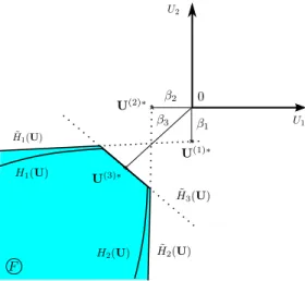
Fig. 3. Illustration of FORM system principle in standard space U1,U2. Three

dependent events define the defect domain F , which is grayed out.

called performance function, is linearized at the most probable fail-ure point U(i)∗. This gives rise to hyper-planes (straight lines in 2 dimensions) whose equation areH

˜

i

(

U

) =

0. U(i)∗ is the closest

point to the origin which respects the constraint Hi

(

U

) =

0. Its

dis-tance from the origin is noted

β

iand called the reliability index. The

FORM method also provides direction cosines:

α

i

= ∇

Hi

(

U(i)∗

)/



∇

H_i

(

U(i)∗

)



. Once all performance functions (n) are treated

sepa-rately, the second stage consists of considering unions or intersec-tions of events, which is the system phase. Let F be the following defect domain: F

=



D



n



i=1 Gi

(

D

) <

0



=



U



n



i=1 Hi

(

U

) <

0



≈



U



n



i=1

˜

Hi

(

U

) <

0



.

(14)

Fig. 3illustrates the FORM concepts in a 2-dimensional standard

U space. The F domain is grayed out. The dependency of different

events, i.e. the orientation of hyper-planes, is taken into account through a covariance matrix defined using direction cosines. The

(

i

,

j

)

-th term of

[

ρ]

is

ρ

_ij

=



α

(i)

_{, α}

(j)



, where

⟨•

, •⟩

is the scalar product. Finally, the defect probability associated with the F do-main is estimated using the n-dimensional multivariate normal cu-mulative distribution functionΦ_n:

PD

=

Prob



_n



i=1 Gi

(

D

) <

0



≈

Prob



_n



i=1

˜

Hi

(

U

) <

0



=

Φ_n

(−β, [ρ]).

(15)

In the case illustrated in Fig. 3, the defect probability is expressed as follows:

PD

=

Φ3

({−β

1

, −β

2

, −β

3

}

, [ρ]).

(16)

Φnis computed thanks to the Genz method [14], which

eval-uates the n-dimensional multivariate normal cumulative distribu-tion funcdistribu-tion almost instantaneously. As limit-state funcdistribu-tions are replaced by hyper-planes, the method gives only an approximation of PD, but it also provides its confidence interval. Again, due to low

part dimension variations in a tolerance analysis context, this lin-earization is often very accurate. This method can easily be applied to compute both defect probabilities PDfand PDagiven respectively

by Eqs.(13)and(2), composed only of event intersections.

Fig. 4. RADIALL coaxial connector scheme. Gaps are emphasized for better

com-prehension. Numbers are the contact point identifications.

Table 1

Dimension characteristics of the RADIALL coaxial connector.

Name Mean Standard deviation

D1 6 0.03 D2 6.1 0.03 D3 12 0.03 D4 12.1 0.03 D5 10.1 0.03 D6 10 0.03 D7 3 0.03

4. RADIALL coaxial connector 4.1. Case study

In this section, a case study is presented, based on an industrial problem. It is a 2D representation of an electric coaxial connector designed and manufactured by RADIALL SA, comprising 2 cylindri-cal parts (seeFig. 4). Due to the presence of gaps in the mecha-nism, part 1 is mobile while part 2 is fixed. The position of part 1 is located in 2D space thanks to the displacement variable vector:

P

= {

X

,

Y

, α}

. Rotational symmetry is taken into account by con-straining

α

positive. Dimensions D are modeled by Gaussian vari-ables and their characteristics are noted inTable 1.

4.2. Assembly defect issue

This coaxial connector can be assembled if the dimensions of part 1 are lower than the corresponding dimensions of part 2, if the following assembly constraints are verified:

m1

(

D

) =

D3

−

D4

≤

0

m2

(

D

) =

D1

−

D2

≤

0 (17)

m3

(

D

) =

D6

−

D5

≤

0

.

The assembly defect probability can be computed thanks to the FORM system method described in Section4:

PDa

=

1

−

Prob

×

(

m1

(

D

) ≤

0

)

(

m2

(

D

) ≤

0

)

(

m3

(

D

) ≤

0

)



Table 2

Assembly issue results for the RADIALL coaxial connector.

Solution method PDain ppm (95% C.I.) Number of calls

(computation time) Monte Carlo simulations 27 490(205) 107_{runs (21 s)}

FORM system 27 380 Analytical result (0 s)

As the functions are independent, the covariance matrix

[

ρ]

is equal to the identity matrix. Thus, Φ3

(−β

1

, −β

2

, −β

3

, [ρ]) =

Φ

(−β

1

)

Φ

(−β

2

)

Φ

(−β

3

)

, with

β

1

=

µ

D3

−

µ

D4

σ

2 D4

+

σ

2 D3

= −

2

.

357

β

2

=

µ

D1

−

µ

D2

σ

2 D2

+

σ

2 D1

= −

2

.

357 (19)

β

3

=

µ

D6

−

µ

D5

σ

2 D5

+

σ

2 D6

= −

2

.

357

.

Finally, PDa

=

1

−

Φ

(

2

.

357

)

Φ

(

2

.

357

)

Φ

(

2

.

357

) =

27 380 ppm

.

(20)

Table 2shows PDaresults computed by MC simulations and by the

FORM system. Both computation methods give comparable results in a very short time because this assembly issue is trivial. However, it is interesting to note that the FORM system methodology provides the exact probability result instantaneously while MC simulations provide a confidence interval on the result.

4.3. Functionality defect issue

Concerning the functionality issue, the non-interference do-mainΩ

(

D

)

is determined by considering each potential contact point. This depends on the mechanism dimensions and defines the admitted positions and orientation P of part 1:

g1

(

D

,

P

) =

D6 2 sin

(α) +

D3 2 cos

(α) −

D4 2

+

X

≤

0 g2

(

D

,

P

) =

D7tan

(α) +

D1 2 cos

(α)

+



D5 2

−

Y



tan

(α) −

X

−

D2 2

≤

0 g3

(

D

,

P

) =

D3 2 sin

(α) +

D6 2 cos

(α) −

D5 2

+

Y

≤

0 g4

(

D

,

P

) =

D6 2 sin

(α) +

D3 2 cos

(α) −

D4 2

−

X

≤

0 (21) g5

(

D

,

P

) =

D1 2 cos

(α)

+



D5 2

−

Y



tan

(α) +

X

−

D2 2

≤

0 g6

(

D

,

P

) =

D3 2 sin

(α) +

D6 2 cos

(α) −

D5 2

−

Y

≤

0 Ω

(

D

) :

P



6



i=1 gi

(

D

,

P

) ≤

0

.

The functional characteristic is Fc

=

α

max. To achieve an

ad-equate electrical connection,

α

max, which represents the largest

α

angle admitted by the mechanism, must not exceed a given thresh-old Fcmax

=

0

.

01 rad. The functional requirement is

α

max

(

D

) =

max

P∈Ω(D)

(α) ≤

F_cmax

.

(22)

To compute PDfwith the proposed method, the preliminary task

is to linearize the initial non-interference constraints g

(

D

,

P

)

in

Eq.(21)with respect to the displacement space P by using a Taylor expansion around a particular point:

(

X

=

0

,

Y

=

0

, α =

Fcmax

)

(to not be confused with the most probable failure point). This point is very pertinent because Fcmax is the angle at which the

functional characteristic value is critical. Then the important con-tact point situations are identified. In 2D space, such a situation has three contact points among the six potential ones (Nc

=

6).

As a consequence, there exist Ns

=

C63

=

20 potential contact

point situations. Five of these are identified thanks to their con-tact point identification, defined inFig. 4in this particular case:

s(1)

_{= {}

₁

_,

₂

_,

₃

_}

_,

_s(2)

_{= {}

₁

_,

₃

_,

₄

_}

_{, s}(3)

_{= {}

₂

_,

₃

_,

₆

_}

_{, s}(4)

_{= {}

₁

_,

₃

_,

₆

_}

and s(5)

= {

2

,

3

,

5

}

as dominant situations. They are obtained us-ing 100 optimization runs. For each of them, a linear problem is solved in order to obtain the P-coordinatesP of these extreme sit-

ˆ

uations. For example, the first one is defined as follows:

ˆ

P1

(

D

) =

P





g

˜

₁

(

D

,

P

) =

0

˜

g2

(

D

,

P

) =

0

˜

g3

(

D

,

P

) =

0

.

(23) Based on these coordinates, 5 performance functions are de-fined:

Li

(

D

) =

Fcmax

−

Fc

(

D

, ˆ

Pi

(

D

)),

i

=

1–5

.

(24)

These functions, although resulting from a linear system, are not linear with regard to D space. Thus, the FORM method transforms them into hyper-planes at the most probable failure point. The in-tersection of events is treated by the FORM system method and PDf

is computed thanks to the multi-dimensional Gaussian cumulative distributive functionΦn. The following equation enables the

com-putation of the defect probability presented Eq.(13):

PDf

≈

5



i=1 Φ4

−

β

(i)

, [ρ]

(i)

 −



i<j Φ8

−

β

(ij)

, [ρ]

(ij)



+ · · · +

(−

1

)

Nds−1Φ 20

−

β

(ij...Nds)

, [ρ]

(ij...Nds)



(25) where

β

(i)

, β

(ij),

β

(ij...Nds),

[

ρ]

(i)

_{, [ρ]}

(ij) _and

_[

_ρ]

(ij...Nds) _{are the}

reliability index vectors and the covariance matrices associated re-spectively with the i-th contact point situation, the i-th and j-th sit-uations and the Ndssituations together. For example, the first term

of Eq.(25)usesΦ4because there is an intersection of Nc

−

3

+

1

=

6

−

3

+

1

=

4 events in the first term of Eq.(13)(Nc

−

6

+

1 in

3 dimensions but Nc

−

3

+

1 in this particular plane model). Thus,

β

(i)_and

_[

_ρ]

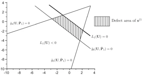
(i)_{are respectively a 4-dimensional vector and square} matrix.

For a better comprehension,Fig. 5 shows the defect area as regards the first identified situation in

(

U1

,

U2

)

space while

(

U3

,

U4

,

U5

,

U6

,

U7

)

are fixed.Fig. 6shows the whole defect area in the

same space. The complete defect area is the union of individual de-fect areas relative to each contact point situation. Some lines can-not be displayed since they are outside the frame. Some lines are also merged with others. It is interesting to note that most defect areas have common limits and are disjoint. Nevertheless, the third and fourth ones have a common intersection. This figure helps to understand the necessity of using the Poincaré formula to compute

PDf (Eq.(13)).

The goal of this application is to show that tolerance analysis can be conducted at a very low computing cost using the FORM sys-tem methodology for simple over-constrained mechanisms with gaps. Different solution methods are proposed based on the two presented methodologies, using both linear and linear non-interference constraints. Results in ppm are listed inTable 3with their 95% confidence intervals (C.I.). Nl

=

107runs were used for

MC, so the 95% C.I. width of PDf is approximately equal to 300

ppm. The FORM system results have also a 95% C.I. due to the Genz method. The low difference between the two MC results shows

Fig. 5. Representation of the defect area of the first contact point situation in standard space U1,U2.

Fig. 6. Representation of the whole defect area in standard space U1,U2.

Table 3

Functionality issue results for the RADIALL coaxial connector.

Solution method PDfin ppm (95% C.I.) Number of calls (computation time)

Monte Carlo with non-linear constraints 47 329(257) 107_{non-linear optimization runs (3 days)}

Monte Carlo with linear constraints 47 202(312) 107_{linear optimization runs (10 h)}

FORM system with linear constraints 47 245(225) 20 FORM solutions+31Φncomputations (10 min)

FORM system upper bound 60 940(136) 5 FORM solutions (3 s)

that non-interference constraint linearization has no measurable impact on PDf. Also, as the FORM system results are very close to

those of MC (Table 3), it shows that the FORM linearization phase has no measurable impact either. This argues that the FORM sys-tem methodology can deal with this kind of problem with a very low computing cost (10 min as opposed to 10 h).

To give an idea of the weight of each dominant contact point situation, the individual defect probabilities associated with each situation were computed as

P_Df(i)

=

Prob



(

Li

(

D

) <

0

)

3



j=1

(˜

gj

(

D

, ˆ

Pi

) ≤

0

)



(26) P_Df(1)

=

30 527

(

65

)

ppm

,

P_Df(2)

=

1861

(

12

)

ppm

,

P_Df(3)

=

13 770

(

27

)

ppm P_Df(4)

=

14 781

(

32

)

ppm

,

P_Df(5)

=

1

(

0

.

01

)

ppm

.

(27) This shows that different situations play a significant role in the defect scenario. Based on these individual situation results, it is possible to compute a PDfupper bound, which is simpler and faster

to obtain, but quite distant from the actual value in this case:

PDf

≤

Nds



i=1

P_Df(i)

=

60 940

(

136

)

ppm

.

(28)

5. Two-axle prismatic joint 5.1. Case study

Now let us consider a second industrial case study, already pre-sented by Ballu et al. [6] and Wu et al. [15]. The new proposed methodology is applied to compute defect probabilities for this mechanism. It is a prismatic joint composed of 2 shafts {3, 4}, one bearing {1} and one other part {2} (seeFig. 7). The axles slide in part {1} and are attached to part {2} by hooping. Part {1} is fixed, while parts {2, 3, 4} are positioned in the vertical direction thanks to displacement variables P

= {

YK

, α}

(see Fig. 7). Parts {2, 3,

4} are designed to move mainly in the horizontal direction, but this study will investigate only vertical displacements, and hori-zontal movements are not considered here. l1

,

l2and l3define the

Fig. 7. Prismatic joint general scheme. Gaps are emphasized for better

comprehen-sion. Numbers are the contact point identifications.

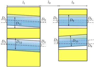
horizontal positions of parts which are fixed. They are modeled by deterministic variables. Due to manufacturing defects, the shafts are not parallel, their borings are not coaxial with them and their dimensions are not at their nominal values. Thus, gaps are intro-duced between shafts and borings, allowing displacements. Di-mensions D characterize relevant manufacturing deviations. D1to D8are the distances between the real axes of the borings and the

shafts at part {1} plane level. D9to D12are the diameters of the

shafts and borings (seeFig. 8). They are modeled by Gaussian vari-ables. D and l characteristics are noted inTable 4.

5.2. Assembly issue

The assembly constraints of this mechanism, obtained geomet-rically, are as follows:

m1

(

D

) =

2D1

−

2

(

l1

+

l2

+

l3

)

l3 D5

−



2

−

2

(

l1

+

l2

+

l3

)

l3



D6

+

D9

−

D11

−

2D3

+

2

(

l1

+

l2

+

l3

)

l3 D7

+



2

−

2

(

l1

+

l2

+

l3

)

l3



D8

+

D10

−

D12

≤

0 m2

(

D

) = −

2D1

+

2

(

l1

+

l2

+

l3

)

l3 D5

+



2

−

2

(

l1

+

l2

+

l3

)

l3



D6

+

D9

−

D11

+

2D3

−

2

(

l1

+

l2

+

l3

)

l3 D7

−



2

−

2

(

l1

+

l2

+

l3

)

l3



D8

+

D10

−

D12

≤

0 m3

(

D

) =

2D2

−

2

(

l2

+

l3

)

l3 D5

−



2

−

2

(

l2

+

l3

)

l3



D6

+

D9

−

D11

−

2D4

+

2

(

l2

+

l3

)

l3 D7

+



2

−

2

(

l2

+

l3

)

l3



D8

+

D10

−

D12

≤

0 (29) m4

(

D

) = −

2D2

+

2

(

l2

+

l3

)

l3 D5

+



2

−

2

(

l2

+

l3

)

l3



D6

+

D9

−

D11

+

2D4

−

2

(

l2

+

l3

)

l3 D7

−



2

−

2

(

l2

+

l3

)

l3



D8

+

D10

−

D12

≤

0 m5

(

D

) =

D9

−

D11

≤

0 m6

(

D

) =

D10

−

D12

≤

0

.

These constraints enable the shafts to penetrate part 1 with-out stress or deformation. To compute PDa, once again both MC

Fig. 8. Prismatic joint notation scheme. Dimensions D1to D8are defined at plane

levels.

Table 4

Dimension characteristics of the prismatic joint.

Name Mean Standard deviation D1,D2,D3,D4,D5,D6,D7,D8 0 0.022 D9,D10 79.78 0.022 D11,D12 80.22 0.022 l1 300 / l2,l3 200 / Table 5

Assembly issue results for the prismatic joint.

Solution method PDain ppm (95% C.I.) Number of calls

(computation time) Monte Carlo simulations 1567(49) 107_{runs (2 min)}

FORM system 1575(73) 1Φ6computation (2 s)

simulations and the FORM system can be used, since the defects do not depend on part positions. The reliability indexes of the FORM system method are computed analytically, since the constraints are linear.Table 5shows the assembly defect results for this case study.

5.3. Functionality issue

The mechanism’s functionality depends on the lower position min

(

YK

)

of point K , belonging to part {2}, in the vertical direction

(seeFig. 7). The functional requirement is that this position be greater than 0.94 mm below its nominal position: min

(

YK

) ≥

YKmin

= −

0

.

94. To compute PDf, the preliminary task is to establish

non-interference constraints. There are 4 potential contact points represented inFig. 7. Each one involves a linearized constraint:

˜

g1

(

D

,

P

) =

YK

+

(

l1

+

l2

+

l3

)α +

D6

+

D9 2

−

D6

−

D5 l3

(

l3

+

l2

+

l1

) −

D1

−

D11 2

≤

0

˜

g2

(

D

,

P

) = −

YK

−

(

l2

+

l3

)α −

D6

+

D9 2

+

D6

−

D5 l3

(

l3

+

l2

) +

D2

−

D11 2

≤

0

˜

g3

(

D

,

P

) =

YK

+

(

l1

+

l2

+

l3

)α +

D8

+

D10 2

−

D8

−

D7 l3

(

l3

+

l2

+

l1

) −

D3

−

D12 2

≤

0 (30)

Table 6

Functionality issue results for the prismatic joint.

Solution method PDfin ppm (95% C.I.) Number of calls (computation time)

Monte Carlo simulations 556(30) 107_{linear optimization runs (28 h)}

FORM system 553(4) 12 FORM solutions+15Φncomputations (5 min)

FORM system upper bound 558(4) 4 FORM solutions (3 s)

˜

g4

(

D

,

P

) = −

YK

−

(

l2

+

l3

)α −

D8

+

D10 2

+

D8

−

D7 l3

(

l3

+

l2

) +

D4

−

D12 2

≤

0 Ω

(

D

) :

P



4



i=1

˜

gi

(

D

,

P

) ≤

0

.

As the displacements are very small, functions are linearized. The defect probability PDfis defined as

PDf

=

Prob



min P∈_Ω(D)

(

YK

(

D

,

P

)) −

YKmin

<

0



.

(31)

This probability can be computed by the first methodology, and by the second one if the contact point situations are well defined. As Ballu et al. [6] did, it is simple to identify them using the iden-tification numbers defined inFig. 7: s(1)

= {

1

,

2

}

,

s(2)

= {

3

,

4

}

,

s(3)

_{= {}

₁

_,

₄

_}

_{and s}(4)

_{= {}

₂

_,

₃

_}

_{. In this case, N}

ds

=

Ns

=

4

,

Nc

=

4.

Thus, the second methodology PDfformulation is as follows:

PDf

=

Prob



₄



i=1



(

Li

(

D

) <

0

)

2



j=1



g_¯s(i) j

(

D

, ˆ

Pi

) ≤

0





(32)

where Li

(

D

) =

YK

(

D

, ˆ

Pi

(

D

)) −

YKmin. Functionality defect

proba-bility results are given inTable 6. As in the previous application, both methodologies give comparable results, but the computation cost of the MC method is significantly higher than that of the FORM system. This application confirms the ability of the FORM system method to deal with functionality issues very efficiently. The de-fect probability of individual situations P_Df(i)

,

i

=

1 to 4, can be com-puted, and their sum gives a PDupper bound, which is very close

to the actual result:

P_Df(1)

=

148

(

1

),

P_Df(2)

=

131

(

1

),

P_Df(3)

=

148

(

1

),

P_Df(4)

=

131

(

1

)

PDf

≈

4



i=1 P_Df(i)

=

558

(

4

)

ppm

.

(33)

This shows that individual defect events are independent in this case.

6. Conclusion

Statistical tolerance analysis is a key step in the design phase for industrial products. Probabilistic approaches provide very use-ful tools for tolerance analysis. The goal is to compute defect proba-bilities of over-constrained mechanisms containing gaps; the latter represent the main difficulty here, since they cannot be modeled as random variables. In fact they are free and have to be considered as deterministic variables. This point greatly complicates the solu-tion process. In addisolu-tion, these kinds of mechanisms are specific, because their non-conformance is caused either by assembly de-fects or by functionality dede-fects. This paper shows that assembly issues are often trivial, whereas functionality issues are complex due to the presence of gaps.

Concerning functionality issues, the paper proposes an innova-tive methodology from the structural reliability domain. The au-thors propose to compute PDf defect probability using the FORM

system method. Several contact point situations are treated sep-arately as dependent events. Their intersection is taken into con-sideration thanks to the multi-dimensional Gaussian cumulative distributive functionΦn, computed by the Genz method. The

pro-posed methodology is compared with another existing method based on MC simulations and optimizations. The two industrial applications show that both presented methodologies give equiv-alent results. The proposed method enables the computation of defect probabilities for mechanisms containing gaps at a very low computing cost (a few minutes compared to several hours). The FORM system methodology is remarkably accurate and can be applied to other mechanisms containing gaps on which several contact point situations can be identified to respect functional requirements. Its efficiency is also linked to the linearity of non-penetration constraints to ensure that extreme functional charac-teristic values are obtained at the contact points.

In the case of more complex mechanisms with gaps whose behavior is governed by highly non-linear functions, the constraint linearization phase could lead to errors in defect probabilities. In future work, it would be interesting to deal with this kind of system.

Acknowledgments

The authors would like to thank RADIALL SA, and particularly Laurent Gauvrit, for their cooperation concerning the presented coaxial connector case study. The Auvergne regional council is also gratefully acknowledged for its financial contribution to this work.

References

[1]Scholtz F. Tolerance stack analysis methods. Boeing Technical Report. 1995. [2]Gayton N, Beaucaire P, Bourinet J-M, Duc E, Lemaire M, Gauvrit L. Apta:

advanced probability—based tolerance analysis of products. Mécanique et Industries 2011;12:71–85.

[3]Nigam SD, Turner JU. Review of statistical approaches to tolerance analysis. Computer Aided Design 1995;27(1):6–15.

[4]Lemaire M. Structural reliability. ISTE, Wiley; 2009.

[5]Qureshi AJ, Dantan J-Y, Sabri V, Beaucaire P, Gayton N. A statistical tolerance analysis approach for over-constrained mechanism based on optimization and Monte Carlo simulation. Computer Aided Design 2012;44(2):132–42. [6]Ballu A, Plantec J-Y, Mathieu L. Geometrical reliability of overconstrained

mechanisms with gaps. CIRP Annals—Manufacturing Technology 2008;57(1): 159–62.

[7]Zou Z, Morse E. A gap-based approach to capture fitting conditions for mechanical assembly. Computer Aided Design 2004;36:691–700.

[8]Ameta G, Davidson J, Shah J. Using tolerance-maps to generate frequency distributions of clearance and allocate tolerances for pin-hole assemblies. ASME Transactions, Journal of Computing and Information Science in Engineering 2007;7(4):347–59.

[9]Dantan J-Y, Qureshi A-J. Worst-case and statistical tolerance analysis based on quantified constraint satisfaction problems and Monte Carlo simulation. Computer Aided Design 2009;41:1–12.

[10]Adragna P-A, Samper S, Favreliere H. How form errors impacts on 2D precision assembly with clearance? Precision Assembly Technologies and Systems 2010;50–9.

[11]Bourdet P, Mathieu L, Lartigue C. The concept of the small displacement torsor in metrology. In: Advanced mathematical tools in metrology II. Series advances in mathematics for applied sciences, vol. 40. World Scientific; 1996. p. 110–22.

[12]Desrochers A. Modeling three dimensional tolerance zones using screw parameters. In: 25th design automation conference. ASME; 1999.

[13]Thoft-Christensen P, Murotsu Y. Application of structural systems reliability theory. Springer-Verlag; 1986.

[14]Genz A. Numerical computation of multivariate normal probabilities. Journal of Computational and Graphical Statistics 1992;141–9.

[15]Wu F, Dantan J-Y, Etienne A, Siadat A, Martin P. Improved algorithm for tolerance allocation based on Monte Carlo simulation and discrete optimization. Computers & Industrial Engineering 2009;56(4):1402–13.