Science Arts & Métiers (SAM)
is an open access repository that collects the work of Arts et Métiers Institute of Technology researchers and makes it freely available over the web where possible.
This is an author-deposited version published in: https://sam.ensam.eu
Handle ID: .http://hdl.handle.net/10985/10316
To cite this version :
Mirko FARANO, Stefania CHERUBINI, Jean-Christophe ROBINET, Pietro DE PALMA - Hairpinlike optimal perturbations in plane Poiseuille flow Journal of Fluid Mechanics Vol. 775, p.R1 -2015
Any correspondence concerning this service should be sent to the repository Administrator : archiveouverte@ensam.eu
Hairpin-like optimal perturbations in plane
Poiseuille flow
Mirko Farano1,2, Stefania Cherubini2,†, Jean-Christophe Robinet2 and
Pietro De Palma1
1DMMM, Politecnico di Bari, Via Re David 200, 70125 Bari, Italy
2DynFluid Laboratory, Arts et Metiers ParisTech, 151 Boulevard de l’Hopital, 75013 Paris, France
In this work it is shown that hairpin vortex structures can be the outcome of a nonlinear optimal growth process, in a similar way as streaky structures can be the result of a linear optimal growth mechanism. With this purpose, nonlinear optimizations based on a Lagrange multiplier technique coupled with a direct-adjoint iterative procedure are performed in a plane Poiseuille flow at subcritical values of the Reynolds number, aiming at quickly triggering nonlinear effects. Choosing a suitable time scale for such an optimization process, it is found that the initial optimal perturbation is composed of sweeps and ejections resulting in a hairpin vortex structure at the target time. These alternating sweeps and ejections create an inflectional instability occurring in a localized region away from the wall, generating the head of the primary and secondary hairpin structures, quickly inducing transition to turbulent flow. This result could explain why transitional and turbulent shear flows are characterized by a high density of hairpin vortices.
Key words: instability, nonlinear instability, transition to turbulence
1. Introduction
Due to their long lifetime, coherent structures determine a large part of the mean properties of transitional and turbulent shear flows, and their generation, instability, and sustainment mechanisms may be useful to explain many details of the dynamics of such flows. Two main examples of coherent structures are streaks and hairpin vortices, which have been observed experimentally and numerically in channel flows, pipe flows, and boundary-layer flows (Singer 1996; Matsubara & Alfredsson 2001; Adrian 2007; Wu & Moin 2009).
Streaky structures are observed at different scales in transitional and turbulent shear flows (Brandt, Schlatter & Henningson 2004; Hwang & Cossu 2010) and their
origin seems now to be well understood. As conjectured by Landahl (1980) some decades ago, elongated near-wall zones of low and high momentum are created by a mechanism of transient growth of the perturbations known as the lift-up effect, linked to the non-normality of the Navier–Stokes operator (Cherubini, Robinet & De Palma 2010b). Such a mechanism is based on the transport of the mean shear by rolls of streamwise vorticity. The quest for the origin of these coherent structures has stimulated the search for perturbations providing maximum amplification in a finite ‘target time’, defined as ‘optimal perturbations’. By optimizing the perturbation energy in a linear framework, several authors have found initial optimal disturbances corresponding to streamwise-elongated rolls inducing streamwise streaks at target time (Butler & Farrell 1992; Luchini 2000). The shape of these optimal perturbations corresponds well to the coherent structures found in transitional and turbulent flows in a low-to-moderate-disturbance environment (Matsubara & Alfredsson 2001). Thus, streaky structures can be explained as the projection of flow disturbances onto the linear optimal flow structure (Luchini 2000).
Also, the mechanism of formation of hairpin vortices has been extensively studied. Wu & Moin (2009) have analysed the generation of hairpin structures from Λ-shaped vortex structures induced in a boundary layer by the receptivity process from large-amplitude free-stream turbulence; Acarlar & Smith (1987) and Henningson, Lundbladh & Johansson (1993) have studied the formation of hairpin vortices from localized disturbances in boundary-layer and channel flows, respectively. Suponitsky, Cohen & Bar-Yoseph (2005) have studied a simple model of interaction between a localized vortical disturbance and a uniform unbounded shear flow, showing that a small-amplitude initial disturbance always evolves into a streaky structure, whereas a large-amplitude one evolves into a hairpin vortex under some conditions. Furthermore, it is well established that hairpin vortices may appear as the consequence of the secondary instability and break-up of elongated streaks (Schmid & Henningson 2001). These and many other studies indicate that, unlike streaky structures, hairpin vortices are generated through nonlinear interactions (Eitel-Amor et al. 2015). The fact that they naturally arise in many transitional and turbulent shear flows, as the consequence of the instability of streaks or induced by other causes (such as roughness elements or flow injection at wall), suggests the existence of a strong energy growth mechanism triggered by nonlinearity. Whether the hairpin vortex might be recognized as an optimal flow structure in a nonlinear energy growth process is the question we want to address in the present paper.
With this purpose, we perform nonlinear optimizations in a simple parallel shear flow such as the plane Poiseuille flow. Nonlinear optimizations in parallel shear flows have been recently performed by Pringle & Kerswell (2010), Monokrousos et al. (2011), Pringle, Willis & Kerswell (2012), Rabin, Caulfield & Kerswell (2012), Cherubini & De Palma (2013) for pipe and Couette flow. In both cases, the nonlinear optimal perturbations were found to induce strongly bent streaks, but hairpin vortices were never observed. However, in those works, optimizations were performed for rather long target times, for which the lift-up mechanism dominates the dynamics. On the other hand, for instance, Karp & Cohen (2014) provide the description of a nonlinear mechanism generating hairpin vortices acting on a time scale which is one order of magnitude smaller. In order to focus our optimization analysis on the generation of the hairpin structure, we choose small target times (O(10h/U), h and U being the reference length and velocity, respectively) and finite-amplitude initial perturbations to rapidly trigger nonlinear effects. In particular, the chosen time scale is typical of the Orr mechanism, much smaller than the typical scale of the lift-up mechanism.
The paper is organized as follows: in §2 we define the problem; then, in §3, we discuss the results; finally, in §4, an outlook is provided.
2. Problem formulation
The Navier–Stokes (NS) equations are solved to compute the flow between two parallel plates, choosing the non-dimensional variables so that half the distance between the plates is h = 1 and the centreline velocity of the laminar flow is Uc= 1. Dirichlet boundary conditions for the three velocity components are imposed at the upper and lower walls of the computational box; whereas periodicity is prescribed in the streamwise and spanwise directions (denoted x and z, respectively, whereas y indicates the wall-normal direction). The streamwise, wall-normal, and spanwise dimensions of the computational domain are 2π, 2, and π, respectively. The NS equations are solved by a fractional-step method with second-order accuracy in space and time (Verzicco & Orlandi 1996), using a staggered grid with 300 × 100 × 120 points, determined by a grid refinement study.
The optimization procedure aims at computing the velocity perturbation u = (u, v, w)T at t = 0 providing the maximum value of a chosen objective function at a given target time, Topt. The objective function is the ratio between the energy density at Topt and the initial (given) one (E(0) = E0), the energy density being defined as:
E(t) =2V1 Z V
(u2+ v2+ w2)(t) dV (2.1) where V is the volume of the computational domain.
The optimization problem is subject to partial differential constraints, namely the nonlinear NS equations in perturbative form. The constrained optimization is performed by a Lagrange multiplier technique coupled with a direct-adjoint iterative procedure using a gradient-based method. For further details about the optimization algorithm the reader is referred to Cherubini et al. (2010a, 2011).
3. Results
We perform nonlinear optimizations of finite-amplitude three-dimensional perturbations for the plane Poiseuille flow, focusing on subcritical values of the Reynolds number, namely, Re = 2000, 3000, 4000, 5000. In order to find optimal perturbations rapidly triggering coherent structures generated by nonlinear effects, we focus on the time scale of the Orr mechanism, preventing the dominant effect of the lift-up mechanism which acts on a much larger time scale. Butler & Farrell (1992) found that the lift-up time scale for the Poiseuille flow at Re = 5000 is about equal to 380. On the other hand, performing several linear two-dimensional optimizations, we have found that the transient energy growth due to the Orr mechanism peaks at t ≈ 10 for all of the considered Reynolds numbers. Thus, Topt = 10 has been chosen for the following nonlinear three-dimensional optimizations. Moreover, using this short target time, we need a sufficiently large initial energy density in order to trigger nonlinear mechanisms. Therefore, several nonlinear optimizations have been performed increasing the value of E0 until, quite suddenly, the initial optimal perturbation localizes in space and the energy gain increases with respect to a linear optimization. Such an increment of the energy gain with respect to the linear case is between 10 % and 30 % for the values of the Reynolds number considered in the present work. The value of E0 has been successively bisected in order to determine
10–5 10–6 10–7 2000 4000 6000 2000 4000 6000 120 100 140 160 180 200 220 Non-linearity threshold Transition threshold Optimization Energy Gain (a) (b)
FIGURE 1. Scaling law for the initial energy (squares), the transition threshold (circles) (a), and the energy gain (b) for the short-time nonlinear optimal perturbation at the nonlinearity threshold.
with an accuracy of two digits the nonlinearity threshold, E0th, i.e. the smallest initial energy at which the nonlinear optimal localizes and the energy gain increases by more than 10 % with respect to the linear value. The values of this energy threshold are shown in figure 1(a) for all of the considered values of Re; they appear well fitted by the scaling law E0th ∝ Re−2.36. The corresponding energy gain at target time obtained by nonlinear optimization is provided in figure 1(b). For all of the considered Reynolds numbers, the energy increases by two order of magnitude in only 10 time units, increasing with Re following the law Re0.84.
It is noteworthy that the value of the nonlinearity threshold is greater than the minimal energy capable of inducing transition, as one would anticipate. For example, we have performed optimizations and bisections for Topt= 50 and Re = 4000, finding a transition energy threshold of about 2.5 × 10⁻⁷ which is one order of magnitude lower than the energy corresponding to the nonlinearity threshold. On the other hand, the energy at the nonlinearity threshold is not very high since we have verified that the linear optimal perturbation rescaled with E0th (see figure 1a) does not lead to transition. In order to evaluate the distance of the nonlinearity threshold from the laminar–turbulent boundary for each optimal perturbation, figure 1(a) also provides the rescaled energy level necessary for placing each optimal perturbation (computed at the nonlinearity threshold) on the laminar–turbulent boundary. Notice that the scaling law for the transition threshold (E(0) ∝ Re−2.35, corresponding about to Re−1.2 for the amplitude) is not far from the value provided by the experimental analysis of Cohen, Philip & Ben-Dov (2009), who found a scaling law for the transition threshold amplitude of A ∝ Re−3/2 using wall-normal flow injection for inducing hairpin vortices.
Figure 2(a) shows the nonlinear optimal perturbation obtained for (Re, E0) = (4000, 2 × 10⁻⁶), composed at t = 0 of several thin tubes of counter-rotating vorticity alternated in the spanwise direction and fully localized in space. The vortices are characterized by a large streamwise vorticity component and are tilted against the base flow, confirming the presence of linear energy growth mechanisms such as the Orr (1907) and the lift-up (Landahl 1980) mechanisms. However, this optimal solution is strongly different from the linear one computed for the same flow due to: (i) its strong localization; (ii) its smaller wavelength in the spanwise direction; (iii) the presence of an inclination of the vortical structures with respect to the streamwise
0 1 2 3 0 2 4 6 0 1 2 0 1 2 3 0 2 4 6 0 1 2 z x y y x z (a) (b)
FIGURE 2. Isosurfaces of the Q-criterion for the nonlinear optimal perturbation obtained with Re = 4000, Topt = 10, and E0 = 2 × 10⁻⁶: (a) t = 0, Q = 0.01 (Qmax = 0.086; red/green surfaces for positive/negative streamwise vorticity values) and (b) t = 10, Q = 0.2 (Qmax= 3.88). 0 1 1 2 2 3 0 0 2 4 6 0 1 2 3 1 2 0 0 2 4 6 0 1 2 3 1 2 0 0 2 4 6 z x y z x y z x y 0 1 1 2 2 3 0 0 2 4 6 0 1 2 3 1 2 0 0 2 4 6 0 1 2 3 1 2 0 0 2 4 6 z x y z x y z x y (a) (b) (c) (d ) (e) ( f )
FIGURE 3. Isosurfaces of the three velocity components: (a,d) u, (b,e) v, (c,f ) w (light grey for positive and black for negative values, u, v, w = ±0.01) of the nonlinear optimal perturbation for Topt= 10: (a,b,c) E0= 2 × 10⁻⁶, Re = 4000; and (d,e,f ) E0= 1 × 10⁻⁵, Re = 2000.
direction. In particular, figure 2(a) shows three pairs of vortices, all of them having different streamwise inclination and length, characterized by a streamwise vorticity of alternating sign. One can observe that the two inner pairs of vortices at the centre of the structure are very close to each other. When such a structure evolves in time, a strong interaction of the vortices occurs immediately after the tilting in the streamwise direction. Therefore, a ‘hot spot’ is created, leading to the formation of the hairpin vortex at target time t = Topt = 10, as shown in figure 2(b). It is also noteworthy that, unlike other parallel shear flows, such as Couette flow (Cherubini & De Palma 2013), this nonlinear optimal structure is characterized by a symmetry with respect to a z = const. plane, which is maintained when the initial energy E0 is increased. We have verified that the optimal perturbation is characterized by this symmetry only for small target times; for target times typical of the lift-up mechanism, the optimal perturbation strongly resembles the one found in Couette flow (Cherubini & De Palma 2013). Figure3(a–c) clearly shows the symmetry of the streamwise and wall-normal velocity components, whereas the spanwise component is antisymmetric with respect to a z-constant axis, recalling the structure of varicose perturbations (Schmid &
150 50 100 200 0 0 50 100 150 200 R.m.s. v elocity Gain t t (a) 100 (b) 10–1 10–2 10–3 10–4 101 100 10–1 10–2 10–3 104 103 102 101 100 105 R.m.s. v orticity
FIGURE 4. Time evolution of the energy gain and velocity (a) and vorticity (b) r.m.s. values for the nonlinear optimal perturbation with Re = 4000, E0= 2 × 10⁻⁶, and T
opt= 10. 0 1 2 0 1 2 0 1 2 0 1 2 0 1 2 0 1 2 1 2 3 1 2 3 1 2 3 1 2 3 1 2 3 1 2 3 0 2 4 6 0 2 4 6 0 2 4 6 0 2 4 6 0 2 4 6 0 2 4 6 x x x x x x z z z z z z y y y y y (a) (b) (c) (d ) (e) ( f )
FIGURE 5. Time evolution of the nonlinear optimal perturbation for Re = 4000, E0= 2 × 10⁻⁶, and Topt= 10. Isosurfaces of Q-criterion ((a–e) Q = 0.02; ( f ) Q = 0.1, green) and streamwise velocity disturbance (u = −0.03, black). Qmax= 0.086, 1.03, 1.99, 7.5, 21.5, 35.4 for (a) to ( f ), respectively. (a) t = 0, (b) t = 5, (c) t = 8, (d) t = 12, (e) t = 16, (f ) t = 40. Henningson 2001). Moreover, it is worth noting that the streamwise and wall-normal components of the velocity clearly show a Λ structure oriented against the flow. This structure, once tilted by the Orr mechanism, becomes a precursor of the hairpin vortex. Very similar structures are found for different Reynolds numbers, as shown in figure 3(d–f ) for Re = 2000, although the latter perturbations are characterized by larger amplitudes (see the scaling in figure 1a).
Direct numerical simulation (DNS) has been employed to study the time evolution of the initial optimal perturbation into a hairpin vortex and its subsequent transition to turbulence. The nonlinear optimal perturbation computed for Re = 4000 with E0 = 2 × 10⁻⁶ has been used to initialize the computation. The results are shown in figure 4 providing the r.m.s. values of velocity (a) and vorticity (b) versus time. It appears that all of the velocity and vorticity components grow together until reaching transition in a relatively short time (at t ≈ 50). It is noteworthy that in other transition scenarios, such as oblique and streaks instability (see Schmid & Henningson 2001), the streamwise velocity experiences a much larger growth than the other components at short times. Snapshots of the time evolution of the vorticity (green) and of the negative streamwise velocity (black) are provided in figure 5. The initial vortex tubes are alternated in z and have opposite inclination with respect to the streamwise direction (see figure 5a), so that the downstream tilting due to the
Orr mechanism has already y
induced at t = 5 the merging of two of these vortices in
a tube of spanwise vorticity resembling a hairpin head (see figure 5b,c). Patches of positive and negative streamwise velocity can be observed in the flow; for t6 Topt they appear rather localized in the streamwise direction (figure 5c) and they elongate in the streamwise direction, creating bent streaks only at times larger than the target time (figure 5d,e). It appears that the hairpin head is originated by a strong localized streamwise velocity defect (Adrian 2007), which is already rather large at t = 0. This defect further increases its amplitude due to the Orr mechanism and to a modified lift-up mechanism (see Cherubini et al. 2011) driven by the initial vortex tubes, until inducing local inflection points in the instantaneous velocity profile.
The dynamics of the nonlinear optimal perturbation shares some important features with the dynamics of the finite-amplitude perturbations analysed by Suponitsky et al. (2005). In particular, they observed the formation of a single hairpin vortex from initial Gaussian vortices of maximum vorticity magnitude Ωmax >1 and streamwise characteristic length L < 5. Such constraints are satisfied by the nonlinear optimal perturbations obtained here which are characterized by Ωmax≈ 1.8 and L ≈ 2.5. Thus, for better analysing the dynamics of the nonlinear optimal perturbation, we have studied the evolution of the main vortical structures in time following the approach of Suponitsky et al. (2005). Let us consider the centre of the vortical structure (CVS), whose coordinates are defined by the following equation:
Xi= Z V Ω2xidV Z V Ω2dV , (3.1)
where Ω is the vorticity magnitude, the denominator is the enstrophy integral, and the index i = 1, 2, 3 represents Cartesian components. To identify the spatial orientation of the vortical structure centred at Xi, we employ the tensor of enstrophy distribution (TED), defined as follows:
Tij= Z
V
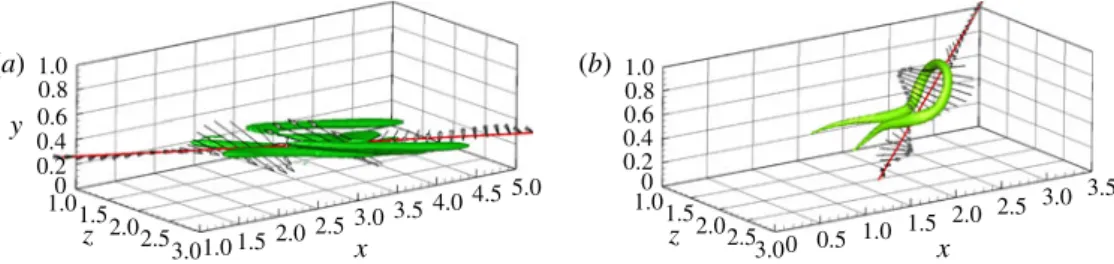
Ω2(xi− Xi)(xj− Xj)dV. (3.2) SinceTij is a symmetric tensor, all its eigenvalues are real. The eigenvector associated with the largest eigenvalue identifies the direction of the principal axis of the vortex, along which the vortex has the largest extension. The insets in figure 6(a,b) show by red lines the principal axis of the vortical structures (represented in green by the Q criterion surfaces) extracted from the DNS at t = 5 and t = 10, respectively. As the flow structures are mainly aligned with the principal axis, we evaluate along this axis the distribution of the streamwise and wall-normal velocity components. The black lines in figure 6(a,b) show such distributions versus the abscissa s along the principal axis (s = 0 at the CVS) at two different times. At t = 5 (figure 6a) we can observe that the velocity components u and v mostly have opposite sign and are equal to zero for s = 0. This behaviour recalls a fundamental feature of eddy motion in wall turbulence; namely, fluctuations have higher probability of spending time in the second (Q2) and fourth (Q4) quadrants of the u–v plane (Adrian 2007), inducing two kind of events: (i) ejections, characterized by negative streamwise fluctuations lifted away from the wall by positive wall-normal fluctuations; (ii) sweeps, characterized by positive streamwise fluctuations being transported toward the wall.
To confirm such a similarity, we have computed the spatial probability density function (PDF) of the perturbation velocity components at different times. Figure 7
–0.20 –0.15 –0.10 –0.05 0 0.05 0.10 0.15 0.20 –0.20 –0.15 –0.10 –0.05 0 0.05 0.10 0.15 0.20 1 –1 0 2 s s (a) (b) 1 – – – 0 2
FIGURE 6. Velocity profile along the principal axis of the TED extracted at two different times from the DNS (black) and the linearized DNS (red), initialized by the nonlinear optimal at (Re, E0)= (4000, 2 × 10⁻⁶). The insets show the Q-criterion surfaces ((a) Q = 0.2 with Qmax= 1.03; (b) Q = 0.3 with Qmax= 3.9; green) and the principal axis (red lines) at two different times. The dot indicates the CVS. (a) t = 5, (b) t = 10.
0.050 –0.050 –0.025 0.025 0 0.050 –0.050 –0.025 0 0.025 –0.050 –0.025 0 0.025 0.050 0.050 –0.050 –0.025 0 0.025 0.050 –0.050 –0.025 0 0.025 0.050 –0.050 –0.025 0.025 0 0.050 –0.050 –0.025 0.025 0 0.050 –0.050 –0.025 0.025 0 –1 –10 –12 –14 –15 –17 –19 –3 –5 –8 –6 (a) (b) (d ) (c)
FIGURE 7. Contours of the logarithm of the probability density function of the wall-normal and streamwise velocity disturbance in a u–v plane (w = 0) for 0 6 y 6 1, extracted at t = 0 (a), 1 (b), 6 (c), 10 (d) from a DNS initialized with the nonlinear optimal with Topt= 10 and E0= 2 × 10⁻⁶. The values of the logarithm of the PDF have been normalized with respect to the total number of points of the computational domain. shows the PDF values (in a logarithmic scale) of the streamwise and wall-normal components of the velocity perturbation, confirming the presence of ejections and sweeps already at t = 0 and up to the time of formation of the hairpin vortex. For instance, in figure 6(a) a sweep is observed upstream of the CVS (s < 0) followed
0 0.2 0.4 0.6 0.8 1.0 0 0.2 0.4 0.6 0.8 1.0 1.01.5 2.02.5 3.0 1.01.5 2.02.5 3.0 1.0 1.52.0 2.5 3.0 3.54.0 4.5 5.0 0 0.5 1.0 1.5 2.0 2.5 3.0 3.5 x x z y z (a) (b)
FIGURE 8. Wall-normal and streamwise components of the velocity vector disturbance along the principal axis of the TED for the nonlinear optimal with E0= 2 × 10⁻⁶: (a) t = 0, (b) t = 14. Isosurface of the Q-criterion ((a) Q = 0.01 with Qmax= 0.086, (b) Q = 4 with Qmax= 12.05).
by a strong ejection and a weak sweep downstream of the CVS (s > 0). At t ≈ 10, the hairpin head is formed downstream of the CVS (s > 0), in correspondence with an ejection, as shown in figure 6(b). This is not surprising since, as found in wall turbulence for a channel flow, the eddy associated with an ejection has a hairpin vortex shape (Adrian 2007). Comparing figure 6(a) and figure 6(b), one can observe that when the hairpin head is formed, the zone of ejection increases its intensity, while the sweep region enlarges in the streamwise direction, reducing its intensity. When the evolution of the same initial perturbation is computed by a DNS based on the solution of the linearized NS equations, the velocity distribution for t > 5 is characterized by increasing values of u and much lower values of v, as shown by the red thin lines in figure 6. Therefore, in the linearized case, streaks with larger intensity will be formed due to the lift-up effect but they will not be associated with wall-normal velocities of opposite signs, rapidly damping the ejection event that is responsible for the lifting of the hairpin head, thus preventing the creation of the hairpin structure.
Figure 8 shows that the alternation of strong sweeps and ejections found at t = 0 is maintained at larger times, thus representing the basic element for the rapid hairpin formation. Moreover, in figure 8(b) one can observe that the hairpin head is placed right in the zone of interaction of the stronger ejection with the stronger sweep, indicating that the formation of the spanwise vortex connecting the initial quasi-streamwise vortices might be a consequence of an inflectional instability taking place in this interaction zone. This observation is in agreement with the minimal flow-element model proposed by Cohen, Karp & Mehta (2014), in which a wavy spanwise vortex sheet was necessary to provide the inflection points for creating hairpin vortices from streamwise counter-rotating vortex pairs.
Figure 9(a,b) provides the instantaneous velocity and vorticity profiles at t = 10, computed solving the nonlinear and the linearized NS equations, respectively, extracted along a vertical axis passing through the hairpin head obtained in the nonlinear case. In figure 9(a) one can observe an inflection point, located at the ordinate corresponding to the peak of vorticity coinciding with the hairpin head (at y ≈ 0.7), in the outer zone of the velocity profile; whereas, in the near-wall region, at y ≈ 0.15, one can observe the deformation of the velocity profile induced by the formation of a negative streak. Inflection points are observed in the linearized case as well (figure 9b), but are placed closer to the wall (y ≈ 0.4), consistent with a shear layer instability induced by a streak. In the nonlinear case, the vorticity peak moves in time towards the centre of the channel, reaching in 10 time units an amplitude
0.2 0.4 0.6 0.8 1.0 0.2 0.4 0.6 0.8 1.0 0 0.5 1.0 1.5 2.0 2.5 3.0 3.5 0 0.5 1.0 1.5 2.0 2.5 y (a) (b)
FIGURE 9. Streamwise velocity (solid lines) and vorticity magnitude (dashed lines) profiles at t = 5 along a wall-normal line passing through the hairpin head computed by the DNS (a) and by the linearized DNS (b), initialized with the nonlinear optimal for E0= 2 × 10⁻⁶. Circles indicate inflection points.
0 0 0 0 1 2 (a) (b) (c) x x y
FIGURE 10. Time evolution of the nonlinear optimal perturbation obtained for Topt= 10 and E0 = 2 × 10⁻⁶ on the plane z = 2. Isosurfaces of the Q-criterion (Q = 0.1, green), isolines of the streamwise velocity disturbance (red positive, black negative), and contours of the wall-normal velocity disturbance (white positive, black negative). Qmax= 0.61, 3.88, 21.52 for (a) to (c), respectively. (a) t = 4, (b) t = 10, (c) t = 16.
almost twice that of the linearized case. When the head of the hairpin is pushed by the wall-normal perturbation toward the centre of the channel, it is advected by the base flow at a higher velocity with respect to the part near the wall, stretching the whole vortical structure in the streamwise direction. Then, due to conservation of circulation, stretching provides a further growth of the vorticity, sustaining the hairpin vortex and allowing secondary hairpin structures to be created (Adrian 2007).
The time evolution of the hairpin structure is shown in figure 10, providing DNS snapshots showing isosurfaces of the Q-criterion (green), isolines of the streamwise velocity disturbance (red for positive and black for negative), and contours of the wall-normal velocity (white for positive and black for negative). One can notice the alternation of patches of u and v with different signs, spread all over the domain, and their effect on the lifting and stretching of the hairpin structure. Nonlinear effects are crucial to sustain the alternation of the u and v perturbation components as well as the vortical structures. This can be clearly inferred by comparing figure 10 with figure 11, showing the time evolution of the nonlinear optimal perturbation obtained by a linearized DNS.
4. Outlook
Nonlinear optimal perturbations having the shape of hairpin vortices at target time have been computed for plane Poiseuille flow, using small target times and finite initial energies. The corresponding initial optimal perturbations are localized in
0 2 4 6 0 0 x x x 0 1 2 y (a) (b) (c)
FIGURE 11. Same as figure 10 but for a linearized DNS. Qmax= 0.79, 0.25, 0.05 for (a) to (c), respectively. (a) t = 5, (b) t = 10, (c) t = 15.
space and composed of spanwise-alternated thin vorticity tubes inclined with respect to the streamwise direction and placed around regions of large streamwise and wall-normal perturbations of opposite sign, resembling localized sweeps and ejections. The streamwise alternation of sweeps and ejections induces strong streamwise velocity defects which generate an inflection point in the velocity profile. Inflectional instability thus creates a spanwise vorticity tube that is lifted and stretched, generating the hairpin head. Transition is triggered suddenly and occurs in a very localized region, already inducing the formation of a hairpin structure at target time (t = 10). The initial flow structure able to create a hairpin vortex in a very short time (t ≈ 10), rapidly leading the flow to turbulence, may be considered as a hairpin precursor, characterized by alternated sweeps and ejections of energy varying with Re−2.36. It appears that, when nonlinear effects are damped, the wall-normal velocity component is not maintained in time, while the streamwise component greatly increases due to the lift-up mechanism, hampering the creation of the hairpin vortex and the subsequent fast transition to turbulence.
In this work we have shown that, for plane Poiseuille flow, a suitable combination of localized sweeps and ejections is capable of maximizing the energy growth in a short time interval, generating a hairpin structure transitioning towards turbulence. Thus, hairpin vortex structures can be the outcome of a nonlinear optimal growth process, in a similar way as streaky structures are linked to a linear optimal growth mechanism. This nonlinear optimal growth process could explain why the final stages of transition to turbulence and turbulent shear flows are characterized by a high density of hairpin structures. Future work will aim at extending these findings to different shear flows, as well as to noisy or turbulent environments.
References
ACARLAR, M. S. & SMITH, C. R. 1987 A study of hairpin vortices in a laminar boundary layer. Part 2. Hairpin vortices generated by fluid injection. J. Fluid Mech. 175, 43–48.
ADRIAN, R. J. 2007 Hairpin vortex organization in wall turbulence. Phys. Fluids 19 (4), 041301.
BRANDT, L., SCHLATTER, P. & HENNINGSON, D. S. 2004 Transition in boundary layers subject to free-stream turbulence. J. Fluid Mech. 517, 167–198.
BUTLER, K. M. & FARRELL, B. F. 1992 Three-dimensional optimal perturbations in viscous shear flow. Phys. Fluids 4 (8), 1637–1650.
CHERUBINI, S. & DE PALMA, P. 2013 Nonlinear optimal perturbations in a couette flow: bursting and transition. J. Fluid Mech. 716, 251–279.
CHERUBINI, S., DE PALMA, P., ROBINET, J.-CH. & BOTTARO, A. 2010a Rapid path to transition via nonlinear localized optimal perturbations. Phys. Rev. E 82, 066302.
CHERUBINI, S., DE PALMA, P., ROBINET, J.-C. & BOTTARO, A. 2011 The minimal seed of turbulent
transition in the boundary layer. J. Fluid Mech. 689, 221–253.
CHERUBINI, S., ROBINET, J.-C. & DE PALMA, P. 2010b The effects of normality and
non-linearity of the Navier–Stokes operator on the dynamics of a large laminar separation bubble. Phys. Fluids 22 (1), 014102.
COHEN, J., KARP, M. & MEHTA, Y. 2014 A minimal flow-elements model for the generation of packets of hairpin vortices in shear flows. J. Fluid Mech. 747, 30–43.
COHEN, J., PHILIP, J. & BEN-DOV, G. 2009 Aspects of linear and nonlinear instabilities leading to transition in pipe and channel flows. Phil. Trans. R. Soc. A 367 (1888), 509–527.
EITEL-AMOR, G., ORLU, R., SCHLATTER, P. & FLORES, O. 2015 Hairpin vortices in turbulent
boundary layers. Phys. Fluids 27, 025108.
HENNINGSON, D. S., LUNDBLADH, A. & JOHANSSON, A. V. 1993 A mechanism for bypass
transition from localized disturbances in wall-bounded shear flows. J. Fluid Mech. 250, 169–207.
HWANG, Y. & COSSU, C. 2010 Self-sustained process at large scales in turbulent channel flow. Phys. Rev. Lett. 105 (4), 044505.
KARP, M. & COHEN, J. 2014 Tracking stages of transition in couette flow analytically. J. Fluid Mech. 748, 896–931.
LANDAHL, M. T. 1980 A note on an algebraic instability of inviscid parallel shear flows. J. Fluid
Mech. 98 (02), 243–251.
LUCHINI, P. 2000 Reynolds-number-independent instability of the boundary layer over a flat surface:
optimal perturbations. J. Fluid Mech. 404, 289–309.
MATSUBARA, M. & ALFREDSSON, P. H. 2001 Disturbance growth in boundary layers subjected to
free-stream turbulence. J. Fluid Mech. 430, 149–168.
MONOKROUSOS, A., BOTTARO, A., BRANDT, L., DI VITA, A. & HENNINGSON, D. S. 2011 Nonequilibrium thermodynamics and the optimal path to turbulence in shear flows. Phys. Rev. Lett. 106 (13), 134502.
ORR, W. M’F. 1907 The stability or instability of the steady motions of a perfect liquid and
of a viscous liquid. Part ii: a viscous liquid. In Proceedings of the Royal Irish Academy, pp. 69–138. JSTOR.
PRINGLE, C. C. T. & KERSWELL, R. R. 2010 Using nonlinear transient growth to construct the minimal seed for shear flow turbulence. Phys. Rev. Lett. 105, 154502.
PRINGLE, C. C. T., WILLIS, A. P. & KERSWELL, R. R. 2012 Minimal seeds for shear flow turbulence: using nonlinear transient growth to touch the edge of chaos. J. Fluid Mech. 702, 415–443.
RABIN, S. M. E., CAULFIELD, C. P. & KERSWELL, R. R. 2012 Triggering turbulence efficiently in plane couette flow. J. Fluid Mech. 712, 244–272.
SCHMID, P. J. & HENNINGSON, D. S. 2001 Stability and Transition in Shear Flows, vol. 142. Springer.
SINGER, B. A. 1996 Characteristics of a young turbulent spot. Phys. Fluids 8 (2), 509–521. SUPONITSKY, V., COHEN, J. & BAR-YOSEPH, P. Z. 2005 The generation of streaks and hairpin
vortices from a localized vortex disturbance embedded in unbounded uniform shear flow. J. Fluid Mech. 535, 65–100.
VERZICCO, R. & ORLANDI, P. 1996 A finite-difference scheme for three-dimensional incompressible
flows in cylindrical coordinates. J. Comput. Phys. 123 (2), 402–414.
WU, X. & MOIN, P. 2009 Direct numerical simulation of turbulence in a nominally