Statistical potentials for evolutionary studies

Statistical potentials for evolutionary studies

par

Claudia L. Kleinman

Département de Biochimie Faculté des arts et des sciences

Thèse présentée à la Faculté des études supérieures en vue de l’obtention du grade de Philosophiæ Doctor (Ph.D.)

en Bioinformatique

June, 2010

c

Faculté des études supérieures

Cette thèse intitulée:

Statistical potentials for evolutionary studies

présentée par: Claudia L. Kleinman

a été évaluée par un jury composé des personnes suivantes: Sébastien Lemieux, président-rapporteur

Hervé Philippe, directeur de recherche Nicolas Lartillot, codirecteur

Mathieu Blanchette, membre du jury Gustavo Parisi, examinateur externe

Joelle Pelletier, représentant du doyen de la FES

Les séquences protéiques naturelles sont le résultat net de l’interaction entre les mé-canismes de mutation, de sélection naturelle et de dérive stochastique au cours des temps évolutifs. Les modèles probabilistes d’évolution moléculaire qui tiennent compte de ces différents facteurs ont été substantiellement améliorés au cours des dernières années. En particulier, ont été proposés des modèles incorporant explicitement la structure des protéines et les interdépendances entre sites, ainsi que les outils statistiques pour éva-luer la performance de ces modèles. Toutefois, en dépit des avancées significatives dans cette direction, seules des représentations très simplifiées de la structure protéique ont été utilisées jusqu’à présent.

Dans ce contexte, le sujet général de cette thèse est la modélisation de la structure tridimensionnelle des protéines, en tenant compte des limitations pratiques imposées par l’utilisation de méthodes phylogénétiques très gourmandes en temps de calcul. Dans un premier temps, une méthode statistique générale est présentée, visant à optimiser les pa-ramètres d’un potentiel statistique (qui est une pseudo-énergie mesurant la compatibilité séquence-structure). La forme fonctionnelle du potentiel est par la suite raffinée, en aug-mentant le niveau de détails dans la description structurale sans alourdir les coûts com-putationnels. Plusieurs éléments structuraux sont explorés : interactions entre pairs de résidus, accessibilité au solvant, conformation de la chaîne principale et flexibilité. Les potentiels sont ensuite inclus dans un modèle d’évolution et leur performance est évaluée en termes d’ajustement statistique à des données réelles, et contrastée avec des modèles d’évolution standards. Finalement, le nouveau modèle structurellement contraint ainsi obtenu est utilisé pour mieux comprendre les relations entre niveau d’expression des gènes et sélection et conservation de leur séquence protéique.

Mots clès : Évolution moléculaire, structure des protéines, Markov chain Monte Carlo, maximum de vraisemblance, statistique Bayesienne, potentiels statistiques.

Protein sequences are the net result of the interplay of mutation, natural selection and stochastic variation. Probabilistic models of molecular evolution accounting for these processes have been substantially improved over the last years. In particular, models that explicitly incorporate protein structure and site interdependencies have recently been developed, as well as statistical tools for assessing their performance. Despite major ad-vances in this direction, only simple representations of protein structure have been used so far. In this context, the main theme of this dissertation has been the modeling of three-dimensional protein structure for evolutionary studies, taking into account the limitations imposed by computationally demanding phylogenetic methods. First, a general statis-tical framework for optimizing the parameters of a statisstatis-tical potential (an energy-like scoring system for sequence-structure compatibility) is presented. The functional form of the potential is then refined, increasing the detail of structural description without in-flating computational costs. Always at the residue-level, several structural elements are investigated: pairwise distance interactions, solvent accessibility, backbone conforma-tion and flexibility of the residues. The potentials are then included into an evoluconforma-tionary model and their performance is assessed in terms of model fit, compared to standard evo-lutionary models. Finally, this new structurally constrained phylogenetic model is used to better understand the selective forces behind the differences in conservation found in genes of very different expression levels.

Keywords: molecular evolution, protein structure, Markov chain Monte Carlo, maximum likelihood, Bayesian statistics, statistical potentials.

RÉSUMÉ . . . v

ABSTRACT . . . vii

CONTENTS . . . ix

LIST OF TABLES . . . xiii

LIST OF FIGURES . . . xv

LIST OF APPENDICES . . . xvii

LIST OF ABBREVIATIONS . . . xix

DEDICATION . . . xxi

ACKNOWLEDGMENTS . . . xxiii

AT A GLANCE . . . xxv

CHAPTER 1: INTRODUCTION . . . 1

1.1 Modeling evolution at the molecular level . . . 1

1.1.1 Models of molecular evolution . . . 7

1.1.2 Towards more realistic models: the case of tertiary structure . . 14

1.2 Evaluating sequence-structure compatibility . . . 22

1.2.1 Physical energies . . . 23

1.2.2 Statistical potentials . . . 26

CHAPTER 2: A MAXIMUM LIKELIHOOD FRAMEWORK FOR PRO-TEIN DESIGN . . . 29

2.1 Background . . . 32

2.2 Results . . . 36

2.2.1 The probabilistic model . . . 36

2.2.2 Statistical potentials . . . 38

2.2.3 Optimizing the potentials by gradient descent . . . 40

2.2.4 Model comparison . . . 44

2.2.5 Specificity of the designed sequences . . . 45

2.3 Discussion . . . 48

2.3.1 Model assessment and comparison . . . 49

2.3.2 Sequence sampling . . . 51

2.4 Conclusions . . . 55

2.5 Methods . . . 57

2.5.1 Structure representation . . . 57

2.5.2 Monte Carlo implementation . . . 57

2.5.3 Likelihood evaluation . . . 58

2.5.4 Model comparison . . . 60

2.5.5 Sequence sampling: site-specific profiles . . . 60

2.5.6 Sequence sampling: Design specificity . . . 61

2.5.7 Learning databases . . . 62

2.6 Additional Files . . . 62

CHAPTER 3: STATISTICAL POTENTIALS FOR IMPROVED STRUC-TURALLY CONSTRAINED EVOLUTIONARY MODELS 65 3.1 Introduction . . . 68

3.2 Methods . . . 71

3.2.1 Statistical potentials . . . 71

3.2.2 Definition and optimization . . . 71

3.2.4 Main chain torsion angles . . . 75

3.2.5 Secondary structure . . . 76

3.2.6 Flexibility of the residues . . . 76

3.2.7 Solvent accessibility . . . 77

3.2.8 Distance-dependent interactions . . . 78

3.2.9 Sequence sampling: site-specific profiles . . . 79

3.2.10 Phylogenetic methods . . . 79 3.2.11 Evolutionary model . . . 79 3.2.12 Bayes factors . . . 81 3.2.13 Datasets . . . 83 3.2.14 Learning databases . . . 83 3.2.15 Phylogenetic datasets . . . 83

3.3 Results and Discussion . . . 83

3.3.1 Definition of statistical potentials and refinement of structural descriptors . . . 83

3.3.2 Site-independent descriptors . . . 84

3.3.3 Pairwise interaction descriptors . . . 87

3.3.4 Combining the potentials . . . 90

3.3.5 Comparison of natural and designed sequences . . . 91

3.3.6 Assessment in a phylogenetic context . . . 94

3.3.7 Transient properties of the SC models . . . 97

3.4 Conclusion and perspectives . . . 99

CHAPTER 4: ASSESSING THE INFLUENCE OF PROTEIN STRUCTURE ON SEQUENCE EVOLUTION: RELATIONSHIP WITH GENE EXPRESSION LEVEL . . . 103

4.1 Introduction . . . 106

4.2.1 Statistical potential . . . 108

4.2.2 Evolutionary models . . . 110

4.2.3 Priors and nomenclature . . . 113

4.2.4 MCMC sampling . . . 113

4.2.5 Datasets . . . 113

4.3 Results . . . 114

4.3.1 Bayes factors . . . 115

4.3.2 Impact of the structural term in the evolutionary model . . . 117

4.3.3 Solvent accessibility is under stronger selection than other struc-tural elements in highly expressed proteins . . . 119

4.4 Discussion . . . 122

4.5 Conclusion . . . 125

4.6 Supplementary figures and tables . . . 126

CHAPTER 5: CONCLUSIONS AND FUTURE DIRECTIONS . . . 129

5.1 Optimization procedure . . . 131

5.2 Structural description . . . 133

5.3 Applications and model extensions . . . 135

2.I Specificity of designed sequences . . . 48

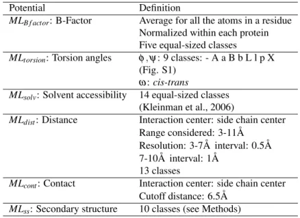
3.I Summary of class definitions used for the various elements of the optimized potentials . . . 84

3.II Bayes factor and optimal β . . . 96

3.III Bayes factors and optimal β for native sequence and rest of the sequences on the alignment . . . 98

4.I Datasets . . . 115

4.II Bayes factors . . . 116

1.1 Sequence conservation mapped onto the crystallographic structure

of thioredoxin 2TRX . . . 15

1.2 Schematic view of force field interactions . . . 24

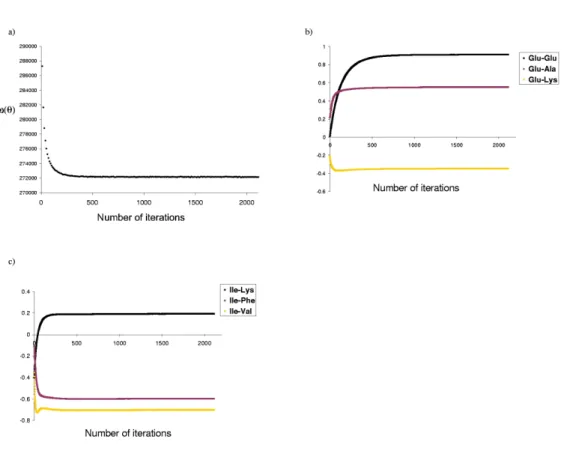
2.1 Convergence of the optimization procedure . . . 43

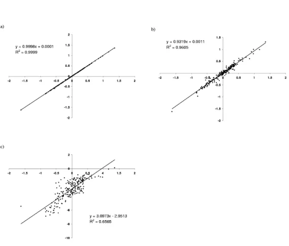
2.2 XY-comparisons of pairwise contact potentials . . . 44

2.3 Effect of the solvent accessibility definition on the potential . . . 45

2.4 Model comparison . . . 46

2.5 Design specificity . . . 47

2.6 Site-specific profiles . . . 54

3.1 B-factor terms . . . 85

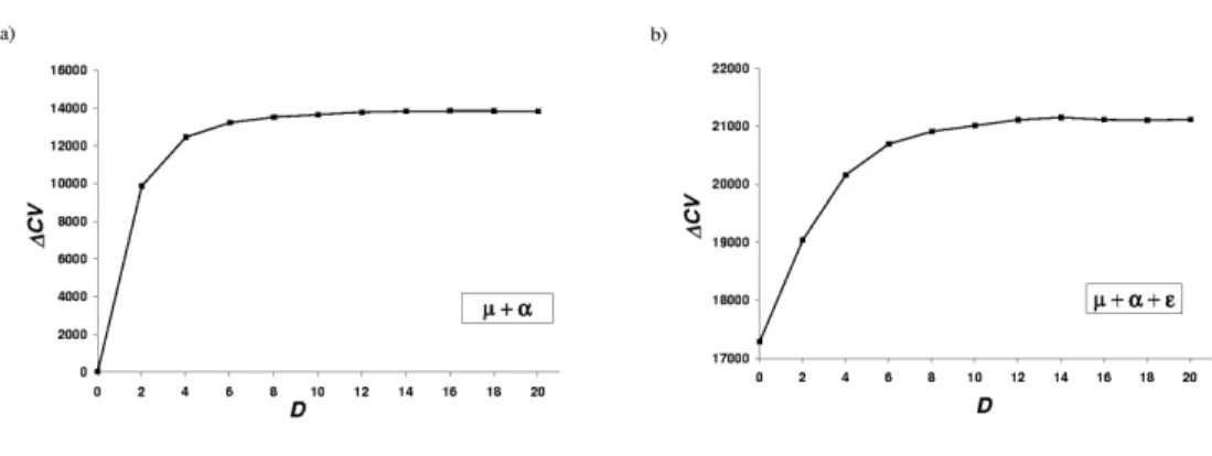
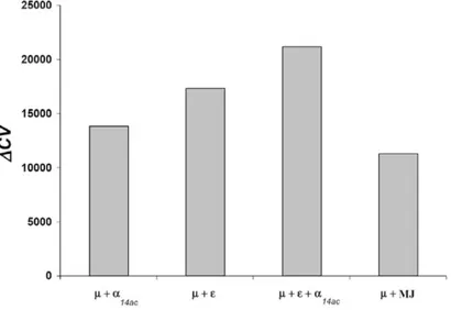
3.2 Cross-validation scores for some of the different potentials obtained 86 3.3 Distance-based pairwise interactions . . . 88

3.4 Sequence logos of site-specific profiles . . . 92

3.5 Stationary Bayes factor as a function of β . . . 99

4.1 Independence of optimal β and size of the dataset . . . 117

4.2 Optimal β under models with or without ω . . . 118

4.3 Optimal β for genes of high and low expression levels . . . 119

4.4 Correlation of optimal β and protein abundance . . . 119

4.5 Posterior distributions of βxin least abundant proteins . . . 120

4.6 Posterior distributions of βxin most abundant proteins . . . 121

4.7 Boxplots of posterior distributions of βx . . . 122

4.8 Starting set of taxa used in the phylogenetic analysis . . . 126

4.9 Independence of optimal β and size of the dataset . . . 126

4.10 Boxplots of optimal β for genes of high and low expression levels 128 4.11 Correlation of optimal β and protein abundance . . . 128

Appendix I: Fast optimization of statistical potentials for structurally constrained evolutionary models . . . xxix Appendix II: Supplementary material for chapter 3 . . . xliii

ADH Alcohol dehydrogenase DS Data set

CV Cross-validation

EM Expectation maximization KLD Kullback-Leibler divergence MCMC Monte Carlo Markov chain

MJ Miyazawa and Jernigan ML Maximum likelihood

MSA Multiple sequence alignment PDB Protein Data Bank

As I write the last lines of this dissertation, I cannot help but thinking of all the people that made it possible. There are many, many people I am grateful to: some of them inspired me, some made these years worth remembering, and some of them helped me through the difficult times.

First, I want to thank my advisor Hervé Philippe for the many things I have learnt from him. The thoroughness when analyzing data, the respect for other’s ideas, the esprit critique, and the constant search for a different angle to look at things. Also, for his patience and support while I was struggling to balance research with family life.

I thank my co-supervisor, Nicolas Lartillot, for his intelligent ideas. Without him, this project would not have even started, let alone succeeded in any way. And, of course, for the opportunity to visit the beautiful France. This work would not have been possible without Nicolas Rodrigue either, who was involved in it from the very first day. I thank him for the knowledge, suggestions and hours of work he invested in this project.

I am especially grateful to Gertraud Burger, who allowed me to land here from the other end of the world. For the hope she had in me even before I could prove anything, and for always showing me nothing but honesty, care and respect.

My sincere thanks to all the people in the Cedergren Bioinformatics Center, who made it such an enriching environment. To Henner Brinkmann, for his help assembling datasets, his cocktails and the countless coffee breaks. To Jean-Christophe Grénier, who was a pleasure to work with, for his contribution to the project as an internship student. To Franz Lang, for his clever and always troubling questions. To Béatrice Roure, Yao-qing Shen, Sivakumar Kannan, Dorothée Coste, Pasha Javadi, Véronique Marie, Fabrice Baro, Shona Tejeiro, Lise Forget and Natacha Beck, for their friendship and support.

The years spent in Montreal would not have been as wonderful without my friends Joannie Roy, Rocío González-Lamothe, Naiara Rodríguez-Ezpeleta, Olivier Jeffroy, Darío Kunik and Marie-ka Tilak. Thanks to them, I have found my home here.

I would like to express my gratitude to Elaine Meunier, Marie Robichaud and Marie Pageau. Their efficiency and kindness made university life much, much easier.

I am also grateful to José María Delfino for welcoming me twice in his lab, for many scientific discussions and invaluable suggestions. And to Javier Santos, whose joy and enthousiasm for research are contagious.

During the development of this dissertation I received financial support from the Natural Sciences and Engineering Research Council of Canada, the biT fellowships for excellence (a Canadian Institutes of Health Research strategic training program grant in bioinformatics), the Bank of Montreal, the Université de Montréal and the Québec Education Ministry. I also acknowledge the Réseau Québécois de Calcul de Haute Per-formance for the computational ressources they provided.

Finally, I am forever indebted to my family. My parents Graciela and Hugo are, of course, ultimately responsible for everything good that came out me. Words of thanks cannot begin to express the gratitude I feel towards them; I hope I made them proud. Thanks to Tito and Nora, for their faith in me and their constant words of encouragement; they meant a lot, each and every one of them. To my three sisters, Popi, Andru and Mailen, who are closer than they think, always on my mind, always in my heart. To my grandmother Chiche, an example of a strong, independent, professional woman. And to Patricia, Roberto, Juan and Angela.

No one, however, helped me more constantly and directly in pursuing this path than Santiago, without whom I would have been lost. During all these years, he has been my Ariadne’s thread, my support and motivation, my guide and inspiration, my everything. Thank you, Doctor.

Just as an archeologist studying ancient buildings to understand human culture, we will look at three-dimensional protein structures to search for clues on the evolutionary processes that shaped them. Imagine for a moment that you find the remains of an unknown civilization. You can learn many things just by looking at the construction materials, from the approximate time this civilization lived to many environmental and social conditions. For example, the fragile materials used in precarious houses of a brazilian favela are impossible to find in a northern canadian home: the rigorous winter weather makes them unfit for survival. Branches, mud and palm leaves belong to a tropical place, and to a certain social class. Big heavy stones and marbles, in turn, point to a complex social organization with division of labour, capable of sustaining constructions over long periods of time.

An archeologist, however, would not stop at the analysis of raw materials. The partic-ular way a construction is made, its organization, its level of complexity, the presence of elements imported from other cultures, all the pieces are essential to the puzzle. When taken together, they speak of social relations, economic systems (nomad or sedentary, agricultural or industrial, producer or consumer). In the same way, we will turn to the buildings in a cell -proteins- to incorporate what we know about them and improve our understanding of the underlying evolutionary process.

But first, we need to determine the elements we will be focusing on. To what level of detail is it worth going into? When are the main traits, such as size, stability, durability of a building enough to draw conclusions, and when is it worth describing detailed features like ornaments and colors? Prisons, hospitals and schools need a particular internal organization, as many enzymes do. For monuments and churches, the exterior counts just as much, as it does in binding proteins. Sometimes, a robust construction is essential: like skyscrapers in earthquake zones, proteins in thermophilic organisms will need an

above-average stability. In other cases, aesthetics and design are the dominant traits. Can we define some general features that are important in all the cases?

The main theme of my PhD work has been the modeling of three-dimensional protein structure in a meaningful way for an evolutionary perspective, while taking into account the limitations imposed by computationally highly demanding phylogenetic methods.

The first chapter presents a general introduction to the concepts from structural and evolutionary biology that are merged in the rest of the work. First, the statistical mod-eling of molecular evolution is introduced, focusing on the description of selective con-straints, in particular those imposed by the protein structure. Then, a discussion on the available tools for evaluating the sequence-structure compatibility follows, from first principles to knowledge-based methods (or statistical potentials), which we chose for our approach.

The second chapter introduces an optimization method of statistical potentials con-ceived for evolutionary studies. In evolution, a protein’s structure changes very slowly, while a multitude of sequences generated by random mutations have to conform to this structure. We thus posed the problem in terms of protein design, or the inverse folding problem, that is, predicting sequences compatible with a given structure. A probabilistic formulation is developed, where the goal is to obtain a probability distribution of se-quences conditional on a structure. An alternative optimization procedure, allowing to considerably decrease the computational time required, is presented in Appendix 1.

In the third chapter, the functional form of the statistical potential is refined, adding several structural elements to the three dimensional description of the proteins and study-ing their impact on the evolution of sequences. To do so, the new potentials are included into a structurally constrained phylogenetic model, and their statistical fit to real data is assessed in a Bayesian framework.

Next, chapter four presents a series of results on the application of this framework to a relatively larger set of proteins, to study the variability of the influence of protein struc-ture on sequence evolution. In particular, we examine how this influence is modulated

by transcriptional properties of the encoding genes, by contrasting patterns of model fit obtained on proteins of different expression level.

Finally, chapter five presents concluding remarks and future directions.

The work presented in this dissertation is previously published in the following arti-cles:

Chapter 2:

C. L. Kleinman, N. Rodrigue, C. Bonnard, H. Philippe, and N. Lartillot. A maxi-mum likelihood framework for protein design. BMC Bioinformatics, 7 :326, 2006.

Appendix 1:

C. Bonnard, C. L. Kleinman, N. Rodrigue, and N. Lartillot. Fast optimization of sta-tistical potentials for structurally constrained phylogenetic models. BMC Evolutionary Biology, 9(1) :227, 2009.

Chapter 3:

C. L. Kleinman, N. Rodrigue, Nicolas Lartillot, and H. Philippe. Statistical poten-tials for improved structurally constrained evolutionary models. Mol Biol Evol, Feb 16. [Epub ahead of print], 2010.

The computational methods for including the potentials into a phylogenetic frame-work and evaluating their model fit are not formally included in this thesis, but published in the article:

N. Rodrigue, C. L. Kleinman, H. Philippe, and N. Lartillot. Computational methods for evaluating phylogenetic models of coding sequence evolution with dependence be-tween codons. Mol Biol Evol, 26(7) :1663-76, 2009.

Finally, the structural analysis performed in the following article was also used to gain insights for the work presented here, but was not included in its totality in this dissertation:

J. Santos, C. Marino-Buslje, C. L. Kleinman, M R. Ermácora, and J.M. Delfino. Consolidation of the thioredoxin fold by peptide recognition: Interaction between E. colithioredoxin fragments 1-93 and 94-108. Biochemistry, 46(17) :5148Ð5159, 2007.

INTRODUCTION

1.1 Modeling evolution at the molecular level

Traditionally restricted to biological classification and descriptive reconstructions of species history, phylogenetic studies have now pervaded almost every discipline in bio-logical sciences; in any comparison of related sequences, there is a phylogeny implicitly assumed. Comparative sequence analysis is routinely used for a range of diverse appli-cations, from the identification of functional regions in genomes (Margulies and Birney, 2008) to structural homology modeling (Madhusudhan et al., 2005). As the amount of public biological data increases, so does the need for a deeper understanding of the dependencies and patterns that originated from a shared evolutionary history.

Studying molecular evolution presents, however, unique challenges. We seek to in-fer the evolutionary scenario most consistent with the incomplete information contained in the data, usually limited to alignments of contemporary sequences; there is virtually no direct information about the past. Furthermore, what makes evolutionary studies particularly difficult (and thus, interesting) is that these observed sequences, as we un-derstand it now, are the net outcome of the interplay of mutation, natural selection and stochastic variation due to genetic drift, with each one of these processes adding a layer of complexity to the problem. Evolution of protein sequences is not determined exclu-sively by selection on protein structure and function, but is also affected by a panoply of diverse, complex, overlapping and sometimes contradictory factors. For example, restricting ourselves to gene features defined at the cellular level and that have been correlated to the rate of protein evolution (reviewed in Pal et al., 2006), we find varia-tions in mutation (Ellegren et al., 2003; Lercher et al., 2001) and recombination (Lercher and Hurst, 2002; Betancourt and Presgraves, 2002) rates associated with genomic

posi-tion, gene dispensability (Hirsh and Fraser, 2001; King Jordan et al., 2002; Wall et al., 2005), protein structure and stability (Haney et al., 1999; Goldman et al., 1998; Dean et al., 2002), position in biological networks (Aris-Brosou, 2005; Fraser et al., 2002) and transcriptional properties, such as expression breadth and expression level (Duret and Mouchiroud, 2000; Subramanian and Kumar, 2004; Wright et al., 2004; Drummond et al., 2006; Drummond and Wilke, 2008).

A great amount of biological knowledge has been built on many of these elements over the last 30 years, which could be potentially included in a comprehensive view of protein evolution. Always with the goal of forming an integral view of protein evolution, one strategy is to tackle one particular aspect at a time. In the present work, we will try to include as much previous knowledge as possible, but only on a subset of all the selective constraints: the ones imposed by the requirements of maintaining a three-dimensional protein structure.

For the challenges described above, probabilistic methods based on explicit models of evolutionary change, along with statistical tools for hypothesis testing, are of par-ticular interest in this field, where traditional evaluation of hypotheses by experimental procedures is almost never an option. For the sake of brevity, and given the broad scope of the subject area, I will focus the discussion on probabilistic methods, and omit the explanation of the alternative parsimony, distance-based and algorithmic approaches to phylogenetic inference. A brief outline is nonetheless presented in Box 1.1; for a thor-ough review, see Swofford et al. (1996) and Felsenstein (2004).

Compared to the alternatives, probabilistic methods present several advantages in our context. The set of assumptions they rely on is made entirely explicit through a model. The laws of probability provide a guarantee that the available empirical evidence (the data) has been analyzed in the framework of this model in a logically coherent fashion. Model violations, given this explicit statement of assumptions, are easier to interpret and evaluate. Finally, model selection theory has a long history in the statistical literature, and several methods have been adapted to the evolutionary problem (Sullivan and Joyce,

2005).

Probabilistic approaches to phylogenetic inference come in two flavors: maximum likelihood and Bayesian approaches. Bayesian approaches of model comparison, which have been extensively developed during the last few years (Box 1.2), are attractive for two main reasons. First, they dispense with the need of analytical integrations by the use of simulation-based numerical strategies as Markov chain Monte Carlo (MCMC). And second, they allow the evaluation of more complex models, since they implicitly penal-ize overly high-dimensional parameterizations by integrating away nuisance parameters (Gelman et al., 2004; Huelsenbeck et al., 2002).

Generally, sequence evolution is described using two components: a phylogenetic tree and a mathematical description of the way individual sequences evolve by nucleotide or amino acid replacement along the branches of that tree (Swofford et al., 1996; Lio and Goldman, 1998; Whelan et al., 2001). These replacements are considered as the product of chance substitution events, and their occurrence at each site is mathematically mod-eled by a Markov process: a stochastic process with a finite number of possible states -the sequence characters at each site- and some known probabilities pi j of moving from

state i to state j on a given time duration. The probability of change of one sequence into another is dependent only on the current state of the system, and not on its previous history; in other words, it is a memoryless process. Defined in this way, the whole pro-cess is entirely specified by the matrix of transition probabilities pi j, which thus takes a

central place in this framework. The development of more accurate and realistic models of sequence evolution has received much attention in recent years, in hopes of reduc-ing phylogenetic reconstruction artifacts due to model misspecifications (Philippe et al., 2005; Lartillot et al., 2007), as well as of addressing particular aspects of molecular evolution (Pal et al., 2006), as I will do in this dissertation.

Probabilistic methods in phylogenetics thus evaluate a hypothesis about evolution-ary history in terms of the likelihood (i.e. the probability) that a proposed model and the hypothesized history would produce the observed data. When phylogeny is the problem of interest, it is then inferred by finding those trees that yield the highest likelihood (Box 1.1). Alternatively, the object of study may be the evolutionary process itself, with the model of sequence change as the hypothesis under scrutiny. In this case, although a joint estimation is possible, a given species’ phylogeny is considered as known to gain insights into the mechanisms of molecular evolution. The observed data thus includes a sequence alignment and the corresponding tree topology, and the probability of a pro-posed evolutionary model given this data is evaluated.

Until recently, the computational cost of probabilistic phylogenetic methods placed severe practical limits on the complexity of the problems that could be handled, forcing

the use of simplifying assumptions that are not always biologically reasonable. This has dramatically changed in recent years with the large increase in computing power, and the parallel development of simulation-based numerical integration strategies like Markov chain Monte Carlo (MCMC). All these tools allow the simultaneous comparison of dif-ferent models, setting the grounds for an iterative research cycle where evolutionary models are progressively refined and contrasted against each other. A greater level of realism is conceivable, dropping some of the simplifications that have been made in the modeling of evolution, among which the independence between sites and the omission of the three dimensional structure of proteins. Before getting into the details, let us overview the most commonly used models of molecular evolution.

Box 1.2: Bayesian model comparison.

Bayesian inference is based on the analysis of the posterior probability distribution over the parameters of interest. Given a model M, with a parameter vector θ ∈ Θ (specifying, for instance, the tree topology and branch lengths, or the parameters of the substitution model, see section 1.1.1), and applied on a dataset D, the posterior probability distribution is given by Bayes’ theorem:

p(θ | D, M) = p(D | θ , M)p(θ | M)

p(D | M) (1.1)

where p(θ | M) is the prior distribution, p(D | θ , M) the likelihood function and p(D | M) =

Z

Θ

p(D | θ , M)p(θ | M)dθ (1.2)

is a normalization constant, also called the predictive probability or marginal likelihood. Parameter estimation is done by computing expectations over the posterior distribution of equation 1.1. In particular,

¯ θ =

Z

θ p(θ | D, M)dθ (1.3)

The analytical calculation of these high dimensional integrals is often not feasible. One way to numerically solve them is to use a Markov chain Monte Carlo walking to sample θ , using the mean of this sample to approximate expectations.

When performing statistical comparisons, the marginal likelihood (1.2) is of primary im-portance. As a function of M, it can be directly interpreted as the likelihood of the model M, given that we observe the data D. The preferred model will be thus the one of greatest marginal likelihood. When two particular models M1 and M2 are being compared, the

Bayes factor in favor of M1 over M2 is defined as the ratio of their respective marginal

likelihoods (Jeffreys, 1935; Kass and Raftery, 1995): B01=

p(D | M1)

p(D | M2)

(1.4) Values of Bayes factor greater than 1 will be considered as evidence in favor of M1, and

vice-versa. The numerical estimation of this value (Neal, 2000; Gelman, 1998; Lartillot and Philippe, 2006) is challenging but feasible; several approximation strategies have been explored for alleviating the computational cost of this calculation (Rodrigue et al., 2007, 2009).

Other approaches for evaluating model adequacy in a Bayesian context are available. In particular, posterior predictive checking has been proposed (Rubin, 1984; Gelman et al., 1996; Rodrigue et al., 2006), where discrepancies between features of true data and data simulated under the model of interest are analyzed. In the work presented in this dissertation, however, we have focused on the traditional Bayes factor, which offers a very intuitive interpretation in a model-selection perspective.

1.1.1 Models of molecular evolution Setting the grounds: DNA models

Models of molecular evolution will be presented in a logical progression, rather than in chronological order of appearance. The simplest models describe evolution as a ho-mogeneous stochastic process that acts on DNA sequences, by accumulating substitu-tions according to a matrix of rates (substitusubstitu-tions per site per unit of evolutionary time) at which a nucleotide is replaced by an alternative nucleotide. By assuming that sites evolve independently, a single character (position) can be considered in isolation from the rest. Further assumptions include time-reversibility and stationarity (that is, a process at equilibrium). Many of these assumptions, necessary at first for rendering the study of molecular evolution into a mathematically tractable form, have been (and continue to be) relaxed, as we will see later.

In its most simple form, the instantaneous rate matrix can be specified with a single free parameter, as is the case in the Jukes-Cantor model (Jukes and Cantor, 1969):

Q_JC=         −3α α α α α −3α α α α α −3α α α α α −3α         (1.5)

where the rows (and columns) correspond to the bases A, C, G and T, respectively, and the (i, j) entry represents the rate at which a base i is replaced by a base j. The process is homogeneous in every possible sense: not only are the rates all equal, but also the matrix remains constant over time and for different sites in the alignment.

Transition probabilities Pab(t) from site a to site b over time t > 0 can be derived

from the instantaneous rate matrix Q. The entries of Q specify the rate of change from state a to state b in an infinitesimal time interval, with diagonal entries chosen so that

the sum of the row elements equals zero (i.e. Qaa = − ∑b6=aQab). P(t) can be derived

solving the differential equation dP(t)/dt = P(t)Q. The solution to this equation, given the start assumption P(0) = I , is the following:

P(t) = etQ= ∞

∑

which can be solved through diagonalization of Q (Lio and Goldman, 1998). Assuming that every site evolves independently, the likelihood of each site is calculated via the pruning algorithm (Felsenstein, 1981), and the full likelihood is subsequently computed by taking the product of each individual site likelihood over all sites in the alignment. The pruning algorithm requires a computational time proportional to the sequence length N, the number of taxa and the square of the number of characters states m allowed at each site (for nucleotide models, m = 4).

The limitations of the extremely simple model in (1.5) are readily apparent, and it has been expanded substantially. Kimura (1980) proposed a two-parameter model that dis-tinguishes between transition and transversion rates; further related contributions consist in considering asymmetries between some of the reciprocal changes (Blaisdell, 1985), a four-parameter (Takahata and Kimura, 1981) and a six-parameter model (Gojobori et al., 1982). Felsenstein (1981) proposed a model in which the rate of substitution to a nu-cleotide depends on the equilibrium frequency of that nunu-cleotide, accounting thus for the nucleotide base composition heterogeneity in DNA sequence data:

Q_F81=         • µ πT µ πC µ πG µ πA • µ πC µ πG µ πA µ πT • µ πG µ πA µ πT µ πC •         (1.7)

dots in the diagonal, and will do so in the subsequent matrices. Hasegawa et al. (1985) combined this model with Kimura’s model by accounting for transition/transversion bias: Q_HKY85=         • β πT β πC α πG β πA • α πC β πG β πA α πT • β πG α πA β πT β πC •         (1.8)

Once again, the rate of exchange between each nucleotide can be further parameter-ized. It is generally convenient to decompose Q into two matrices, (ρ) and (π), repre-senting the exchangeability parameters and the equilibrium frequencies, respectively. In the most general case of these kind of DNA models, these matrices are:

(ρ) =         • ρAC ρAG ρAT ρCA • ρCG ρCT ρGA ρGC • ρGT ρTA ρTC ρT G •         (1.9) and (π) =         πA 0 0 0 0 πC 0 0 0 0 πG 0 0 0 0 πT         (1.10)

where ∑1≤m≤4πm= 1. The diagonal elements of Q are then equal to the

are once again set such as the sum of the elements of each row equals zero. Constrain-ing Q into a symmetric matrix such that ρlm= ρml ensures time-reversibility and yields

the GTR (General time-reversible) model. This is the model that will be used later on as a basis (describing the mutational process) for constructing a mechanistic model of the mutation-selection process that operates on the evolution of protein sequences. Al-though this parameterization does not reflect tendencies for mutation rates to be context-dependent, it constitutes a good compromise between accuracy in the description of the mutational process and conceptual simplicity, important in this stage of model develop-ment. More realistic treatments of the mutation process could be added in a later stage.

Considering protein phenotype: amino acid models

A first direction to more explicitly incorporate selective effects on the substitution process of protein genes is to model evolution directly at the amino acid level, where the phenotypic expression of a genetic change is most evident. Substitutions that change the amino acid sequence should have a more drastic effect on phenotype, and a lower probability of fixation for molecules under purifying selection. A large body of empirical evidence shows that the rate of exchange between different amino acids is affected by the physicochemical characteristics of the amino acids involved, and this effect is very difficult to capture with a DNA model that treats all sites as equal, without regard to the amino acid sequence encoded.

Formally, amino acid models of sequence evolution are similar to the nucleotide models described so far, but with a state space of 20 characters instead of 4. In contrast with DNA substitution models, however, empirical matrices are generally used, which at first have been obtained by counting pairs of amino acids at homologous positions in large sets of aligned proteins (Dayhoff et al., 1978; Jones et al., 1992b). More recently, matrices optimized by maximum likelihood have also been proposed for mitochondrial (Adachi, 1996), chloroplast (Adachi et al., 2000), and nuclear (Whelan and Goldman, 2001) proteins. Typically, a hybrid model is used in the phylogenetic analysis of amino

acid sequences: equilibrium frequencies are estimated from the analyzed data, while the exchangeability parameters are taken from one of the empirical models described above.

Including the genetic code: codon models

The effects of effectively changing the amino acid sequence by a site substitution are better captured by approaches based on amino acid models than with a nucleotide-based model. However, the former have the drawback of not taking into account the genetic code structure and of confounding mutation and selection, by only analyzing the net effect of these two complex processes. A third class of models, formulated at the codon level, circumvent these two limitations.

In order to accommodate the structure of the genetic code, the definition of a site (that is, the unit of substitution) is changed from single nucleotide to triplets of nu-cleotides. A distinction is made between substitutions that change the encoded amino acid (nonsynonymous) and the ones that do not (synonymous). Assuming that synony-mous substitutions are neutral, codon evolution is thus described as a combination of changes at the nucleotide level and selective constraints operating at the protein level.

The most widely used codon models are modifications of those originally proposed by Muse and Gaut (1994) and Goldman and Yang (1994). In both cases, instantaneous changes at more than one codon position are disallowed, as well as changes to premature stop codons. The state space of these Markov models is thus increased to the 61 sense codons of the universal genetic code. The original formulation of Muse and Gaut (MG) has a rate matrix of the form

QMGab =             

0 if a and b differ by more than one codon position α πb synonymous substitution

β πb nonsynonymous substitution

The parameter π_b, representing the equilibrium frequency of the nucleotide type in the target codon, accounts for compositional heterogeneity at the nucleotide level. At the phenotypic level, this model allows for a different rate of substitution for synonymous (α) and nonsynonymous (β ) events.

In the Goldman and Yang (GY) model, the equilibrium frequency of the target codon (as opposed to nucleotide type) is used to describe constraints at the DNA level (noted here π_c(b)). A parameter accounting for transition/transversion bias (κ) is included. To account for selective constraints at the amino acid level, substitution rates are modified by a multiplicative factor in the case of a nonsynonymous event. The definition of these factors is based on an amino acid distance matrix, derived by comparing physicochemi-cal properties of the 20 amino acids (Grantham, 1974). The off-diagonal elements of the rate matrix are defined as follows:

Q_GYab=             

0 if a and b differ by more than one codon position µ πc(b)e−dAAaAAb/V aand b differ by a transversion

µ κ πc(b)e−dAAaAAb/V aand b differ by a transition

(1.12)

where dAAaAAb is the physicochemical distance between amino acids a and b, and

V is a tuning parameter allowing the distance matrix to better fit the data, accounting for differing levels of sequence variability between genes. This model was later simpli-fied by the authors to estimate selective pressure explicitly using the single parameter ω (Yang, 1998). This is essentially equivalent to the treatment in the MG model, setting α = µ and β = µ ω . If frequent amino acid changes present a selective advantage, the nonsynonymous substitution rate will be higher than the synonymous rate, and as a re-sult ω > 1. Conversely, the case where purifying selection acts to preserve amino acid sequence corresponds to ω < 1. Neutrally evolving sequences exhibit similar

synony-mous and nonsynonysynony-mous rates, and thus ω ≈ 1. The simplified version of this model is thus: Q_GYab =                           

0 if a and b differ by more than one codon position µ π_c(b) aand b differ by a synonymous transversion µ π_c(b)κ aand b differ by a synonymous transition µ π_c(b)ω aand b differ by a nonsynonymous transversion µ π_c(b)κ ω aand b differ by a nonsynonymous transition

(1.13)

Codon models formulated in this way have direct connections to population genetic theory (Thorne et al., 2007; Yang and Nielsen, 2008). If the rate of a sequence change can be separated into factors corresponding to mutation (Qmut) and to natural selection, then the factor associated with natural selection represents the probability of fixation. For a population of size ℵ, we have, at the population level:

Q_ab= 2ℵQmut_ab p_{f ix}(ab) (1.14)

Since a neutral substitution in a diploid population has a probability of fixation

p0_{f ix}(ab) = 1

2ℵ (1.15)

We can write the rate of substitution from a to b as:

Q_ab= Qmut pf ix(ab) p0_{f ix}(ab)

!

(1.16)

In this way, the selective parameter ω of equation 1.13, as well as the term e−dAAaAAb/V

particu-larly attractive for our purposes, that is, assessing selective constraints related to the protein structure. In addition to providing an improvement in model realism for protein coding sequences, codon models can also be designed to test hypotheses about the se-lective pressures operating on sequences (reviewed in Delport et al., 2009; Anisimova and Kosiol, 2009).

Although the codon models presented so far are mechanistically motivated, in the sense that translation of proteins is explicitly considered via the genetic code structure and the separation of processes acting at the DNA and amino acid level, only the net resultant of selection is captured in the parameters modulating nonsynonymous substi-tutions. Our motivation in the present work, however, is to focus exclusively in the constraints imposed by the three dimensional structure, in order to disentangle these structural constraints from other selective forces.

Increasing the state space in codon models produces high computational demands, which has prevented their widespread use for phylogenetic inference and the develop-ment of more complex versions of these first models. This has started to change in recent years, and several extensions relaxing some of the initial simplifying assumptions have been proposed (reviewed in Anisimova and Kosiol, 2009), allowing for the development of a mechanistic modeling alternative with explicit consideration of protein structure, as we will see in section 1.1.2.

1.1.2 Towards more realistic models: the case of tertiary structure

Proteins require a suitable three dimensional structure to function. Substitutions that affect the stability of the folded state will have a deleterious effect on fitness, and a lower probability of fixation. Stability of the native state is not, however, the only structural requirement of a viable molecule. For example, exposure of particular combination of amino acids on the surface, enabling the protein to interact inappropriately with a

Figure 1.1: Sequence conservation mapped onto the crystallographic structure of thioredoxin 2TRX. Sequence profiles generated from a multiple sequence alignment (MSA) of 162 eukaryotic sequences, as described in chapter 3. The frequency of the 20 amino acids a at each position i was computed, yielding a vector qi(a) of site-specific

profiles. In the graphic representation, the total height hiat each position is proportional

to the Shannon information as follows: hi= ∑aqi(a)lnqi(a). These Shannon

informa-tion scores were then mapped on the protein structure according to the color scheme on the right. Secondary structure representation taken from PDBsum (Laskowski, 2009). Bottom: native sequence of the reference structure, from E. coli.

wide range of cellular components may induce aggregation (Bucciantini et al., 2002; Dobson, 2003), causing unspecific cellular toxicity. In another example, flexibility and mobile regions are important for the function of an enormous number of proteins (see for example Gerstein and Echols, 2004; Wilson and Brunger, 2000; Huse and Kuriyan, 2002).

All these requirements produce heterogeneous substitution processes across sites that are evident at first sight in the alignments of homologous sequences; an illustration is presented in figure 1.1. Some of the positions owe their level of conservation to con-straints related to the specific function of the protein (e.g. active site of the enzyme or ligand binding sites). Some others, on the contrary, are conserved because of the structural role they play in the molecule. Such is the case of the two prolines in this particular sequence: Pro40 produces a bending in a long alpha helix, while Pro76 is found in a particular conformation, favoring the establishment of the alpha helix that follows. The conservation of glycines is due to their lack of side chain, which allows them to adopt extreme conformations of their backbone angles (for example, Gly84 and Gly92), or to be accommodated in a very reduced space (Gly33). In another example, a polar interaction between Asp26 and Lys57 explains the amino acid profile observed at these positions. All this information we obtain by analyzing the structure testifies to the intimate relationship between structural role and evolutionary conservation.

From the early substitution models that considered evolution of sequences as the result of a homogeneous, purely neutral evolutionary process, models of molecular evo-lution have been improved substantially by including a variety of biological phenomena. Practically all the assumptions made for the Jukes-Cantor model (1969) have been re-laxed in subsequent works, for the three types of sequence data (nucleotide, codon and amino acid). For example, heterogeneity in the substitution process, both across sites (see below) and over time (Yang and Roberts, 1995; Galtier and Gouy, 1998; Galtier, 2001; Huelsenbeck, 2002; Foster, 2004; Blanquart and Lartillot, 2006; Boussau and Gouy, 2006; Gowri-Shankar and Rattray, 2007; Zhou et al., 2010), has been introduced

in a number of models, producing almost invariantly an improvement in terms of fit. Once again, we are interested in selective constraints pertaining to the protein struc-ture, so I will focus on model extensions to address them, and omit details on the rest. As shown in figure 1.1, tertiary structure induces heterogeneity in the substitution pro-cess across sites. The first significant improvement in evolutionary models implicitly addressing this issue was the introduction of the rates across sites models (Olsen, 1987; Yang, 1993, 1994, 1996), where the rate of evolution is represented by a random variable drawn from a gamma distribution, or a discrete version of this distribution with a lim-ited number of classes. In a similar perspective, the ω parameter of codon models can be drawn from various probability distributions to describe among-site variation of selective pressure (reviewed in Anisimova and Kosiol, 2009). In the simplest versions, a prespec-ified number of site classes is used (typically 3: positive selection, neutral and negative selection). Discrete versions of continuous distributions or distribution mixtures have also been applied (Yang et al., 2000; Pond and Muse, 2005). Yang and Swanson (2002) implemented models for prepartitioned datasets, for the case where prior information is available to partition sites in the protein into different classes. In another approach, Huelsenbeck et al. (2006) proposed the use of a Dirichlet process prior to model site-specific variation of ω; under this process, the number of classes is not predetermined, but it is instead a random variable controlled by a parameter estimated from the data.

In all the modeling alternatives described so far, however, only the overall rate of substitution but not the remaining parameters of the evolutionary model (equilibrium frequencies and relative rates of substitution) are allowed to vary across sites. We know, however, as illustrated in figure 1.1, that the heterogeneity in the substitution process is evident not only in the number of nonsynonymous substitutions, but also in the na-ture of these substitutions. This is the case for the stabilizing polar interaction between Asp26 and Lys57, which induces a particular amino acid profile for those positions in the alignment. Or for Leu99 and Leu103, whose importance for establishing the hydropho-bic core of the molecule (Santos et al., 2007) prevents the fixation of non-hydrophohydropho-bic

residues at these positions. A number of evolutionary models allowing consideration of changes in the substitution process (other than the rate parameter) have been proposed. In the model proposed by Bruno (Bruno, 1996; Halpern and Bruno, 1998), a vector of amino acid equilibrium frequencies specific for each site is considered. This approach requires a very large number of species in the alignment, since the amino acid frequen-cies have to be estimated for each column. The CAT model (Lartillot and Philippe, 2004), a mixture model allowing for a finite number of classes characterized by its own set of equilibrium frequencies, proved to be a more reasonable approach. In this model, a Dirichlet process prior is used to estimate the total number of classes and their respec-tive amino acid profiles, with the class assigned to each site also a free parameter of the model. This approach has been recently implemented at the codon level (Rodrigue et al., 2010).

Explicit treatment of protein structure

The models described so far are phenomenological in nature: they capture substitu-tion patterns through parameters estimated from the data, without an explicit modeling of the underlying causes (Rodrigue and Philippe, 2010). In the work presented here, on the contrary, we want to explore a mechanistic alternative, where prior knowledge on protein structure is directly incorporated, with the belief that the insights and advances of the structural biology community over the last years should help improving our un-derstanding of sequence evolution.

Several attempts have been made to model evolution at the amino acid level with explicit treatment of structural constraints. Relaxing the assumption of a single ex-changeability matrix for all sites, substitution matrices specific for predefined structural classes have been proposed (Overington et al., 1990; Wako and Blundell, 1994a,b; Koshi and Goldstein, 1995), with the implicit assumption that the structural environment of a residue is the main force acting on the evolution of this site. Dimmic et al. (2000) have extended this model, using a fitness function different for each one of a fixed number

of classes, where each site’s class is a priori unknown. The relationship of the site classes with the protein structure is however not clear, because the many selective con-straints operating at different sites are confounded. As a result, the correlation of the optimized fitness parameters of the model and the biophysical characteristics of amino acids is poor, and the interpretation of the fitness classes obtained is not evident. Thorne, Goldman and coworkers proposed probabilistic models where a Markov chain describes features of the secondary structure of proteins, and each category of structural environ-ment uses a different Markov process model of amino acid replaceenviron-ment (Goldman et al., 1996; Thorne et al., 1996; Lio et al., 1998). The models provide an improvement in the description of the evolutionary process. However, only extremely simple structural representations have been used, namely a few categories of secondary structure and two states for solvent accessibility.

More importantly, all of the models described so far make the assumption of inde-pendence between sites, a simplification invoked for computational reasons but incom-patible with a realistic treatment of the protein structure. It was not until recently that site interdependencies could be treated within a standard phylogenetic framework, which is the subject of the next section.

Structurally constrained evolutionary models

Modeling site dependencies in a probabilistic phylogenetic context is not a trivial task. Likelihood calculations using Felsenstein’s pruning algorithm (Felsenstein, 1981) require the determination of transition probabilities between states, which involve rate matrix exponentiation (equation 1.6). When considering general site dependencies, the rate matrix is no longer a 4x4, a 20x20, nor even a 61x61 matrix. If we assume that a sub-stitution at one site may affect any other site in the molecule (which is not a very bold as-sumption from a biological perspective), the Markov process specified at the codon level is, in fact, equivalent to the process generated by a 61Nx61N matrix, with single entries describing rates of change from one N-codon sequence to another. The computational

cost of numerically calculating the transition probabilities with these high dimensional matrices is prohibitively expensive, and has justified the assumption of independence between sites usually invoked in phylogenetic methods.

Alternative techniques of likelihood calculations for evolutionary inferences deal-ing with dependence among changes at different positions have recently been proposed (Jensen and Pedersen, 2000; Hwang and Green, 2004; Siepel and Haussler, 2004; Chris-tensen et al., 2005). Matrix exponentiation when calculating transition probabilities (equation 1.6) aims at integrating over all possible substitution histories, over a given phylogenetic phylogenetic tree. An alternative way of calculating this integral is to use MCMC to directly sample the complete substitution history, estimating in this way the value of this integral. Although still computationally demanding, the problem becomes now tractable.

These approaches were formulated to deal with context-dependent mutation, but Robinson et al. (2003) adapted the ideas of Jensen and Pedersen (2000) to the case where general dependencies are due to natural selection on phenotype, to explicitly model structural constraints within a standard phylogenetic framework. Their description of structural constraints is based on the work of Parisi and Echave (2001), who developed a technique for simulating the evolution of sequences that conform to a known tertiary structure. In this model, a scoring system for sequence-structure compatibility is used to evaluate the probability of fixation of a given mutation, assuming a coarse-grained pro-tein structure that is constant through evolution. Nonsynonymous changes that make the sequence less compatible with the protein structure (for example, by introducing desta-bilizing interactions) will have a lower rate of occurrence. Formally, the instantaneous rate matrix originally proposed by Robinson et al. (2003) has the form

Q_DEPab =                           

0 if a and b differ by more than one codon position µ π_c(b) for a synonymous transversion

µ π_c(b)κ for a synonymous transition µ π_c(b)ω eβ ∆E(a,b) for a nonsynonymous transversion µ π_c(b)κ ω eβ ∆E(a,b) for a nonsynonymous transition

(1.17)

Except for the term related to the protein structure in nonsynonymous rates, the parameterization is equivalent to the GY model described in equation 1.13. Parame-ters associated to the mutation process include the nucleotide equilibrium frequencies (πi)1≤i≤4, the transition/transversion rate κ, and the parameter µ to scale the overall rate

of change.

As for selective constraints acting on nonsynonymous changes, two terms are in-volved. The parameter ω, formulated in the same spirit as in the GY model, is intended to capture contributions to nonsynonymous rates that are not exclusively related to the protein structure. The innovation of this model lies in the term eβ ∆E(a,b)_{, describing}

the effects of constraining the sequences to a particular protein structure. This term has two components. For a proposed sequence s, E(s) measures how well s fits the protein structure. In their original formulation, Robinson et al. (2003) used a statistical poten-tial originally derived for the protein-fold prediction problem (Jones et al., 1992a). The development of an accurate sequence-structure compatibility score for this type of evo-lutionary models is the main subject of this dissertation, so I will save the details for next sections. The second component of the structural term in this model, β , is treated as a free parameter, and estimated from the phylogenetic data along with the others. It represents the strength of selection for structural compatibility: when β = 0, the model simplifies to the widely used GY codon model (equation 1.13). Biologically reasonable

values of β are positive, corresponding to the case where evolution favors substitutions that fit the structure better. The higher the value of β , the stronger the role the structural term plays in the evolutionary model.

The focus of the works of Parisi and Echave (2001) and Robinson et al. (2003), and the subsequent work of Rodrigue and coworkers (Rodrigue et al., 2005, 2006, 2007) was on the definition of the evolutionary model and the statistical tools to perform phyloge-netic inference and model comparison dealing with site dependencies. The sequence-structure compatibility measure, however, was to some extent neglected. In its most complex form, an empirical potential originally derived for the protein-fold prediction problem (Jones et al., 1992a) was used, consisting in two components: one account-ing for solvent accessibility requirements, and the other related to pairwise interactions between residues close in space. Since, in contrast to the phenomenological models pre-sented in previous sections, this approach attempts to provide a mechanistic description of the way natural selection operates on the evolutionary process, the accuracy of the model will be highly dependent on how this mechanistic description matches reality. In the following chapters, we will concentrate on ways of measuring how well a sequence fits a structure, and how this measure can be improved without incurring in excessive computational costs.

1.2 Evaluating sequence-structure compatibility

In the phylogenetic framework just described, each mutation undergone by a protein during evolution has to be evaluated for its compatibility with the structure and con-trasted with all the other possible mutations, assuming that the tertiary structure remains invariant. This formulation presents important analogies to the protein design problem, where the goal is to find sequences that fold into a given conformation. Since the size of both the sequence and conformational space are extremely large, there is a trade-off between accuracy and speed when evaluating each sequence, and protein design

ap-proaches use several strategies to speed up the scoring process. This trade-off is even more pronounced in the phylogenetic context, because of the additional computational burden involved in calculating likelihood scores.

There are two very different types of scoring functions currently used. The first ones are physical energies that can be obtained, in principle, from a fundamental analysis of forces between particles. The second ones, called statistical potentials, work with simplified versions of the proteins, and their parameters are derived from known protein structures.

1.2.1 Physical energies

Semi-empirical potentials, widely used to perform molecular mechanics calcula-tions, such as CHARMM (Brooks et al., 1983), AMBER (Cornell et al., 1995) and OPLS (Jorgensen and Tirado-Rives, 1988), work at the atomic level. They consist of a mathematical expression of the energy of a system as a function of the cartesian coor-dinates of the atoms (−→R). Although quantum mechanical calculations can yield potential surfaces for small molecules, it is not yet feasible to calculate directly such surfaces for large macromolecules. Semi-empirical approaches work, instead, with a fairly simple, though atomically detailed, ‘ball and spring’ type models: atoms are represented as spheres with point charges, with chemical bonds treated as springs. In addition to the atomic coordinates, thus, the energy value also depends on a set of parameters that de-scribe the geometric and energetic properties of interactions between particles, adjusted to optimize agreement with experimental data and with quantum calculations on smaller molecules (Karplus and Petsko, 1990; Ponder and Case, 2003; Guvench and MacKerell, 2008). The combination of the mathematical function and the parameters is commonly referred to as a “force field”.

Figure 1.2: Schematic view of force field interactions. Covalent bonds are indicated by heavy solid lines, nonbonded interactions by a light, dashed line. Figure from Ponder and Case (2003).

The most commonly used protein force fields incorporate a relatively simple poten-tial energy function (Ponder and Case, 2003):

V(−→R) =

_∑

_∑

_∑

_∑

The first three summations are over bonds (interactions between atoms 1-2 in figure 1.2, angles (interactions between atoms 1-3), and torsions (between atoms 1-4). The final sum, over all pairs of atoms i and j, describes electrostatics that use partial charges qion

each atom that interacts via Coulomb’s law. The combination of dispersion and exchange repulsion forces are represented by a Lennard-Jones 6-12 potential; this is often called the ’van der Waals’ term. Equation 1.18 is about the simplest potential energy function that can reproduce the basic features of protein energy landscapes at an atomic level of detail (Ponder and Case, 2003).

When calculating the energy of a protein upon mutation, two main requirements of such detailed molecular representation involve high computational costs. First, the po-sition of every atom of the new sequence has to be determined. Even when reducing the conformational search by assuming a fixed backbone, we still have to face the

prob-lem of positioning side-chains. The complexity of this search can be further reduced through the use of rotamer libraries (collections of statistically preferred side chain con-formations for each residue type (Tuffery et al., 1991; Dunbrack and Karplus, 1993), but it still implies large computational times, and the energy function has to be adjusted ad hoc to accommodate such simplifications. Second, there is a need for an accurate treatment of the solvent environment, which adds a significant number of atoms to the system. Such treatment may be performed using explicit (that is, modeling separately each solvent molecule) or implicit models (Roux and Simonson, 1999), with the former being a more microscopically complete method while the latter having the advantage of savings in computer time. For the CHARMM potential, for example, the calculations with explicit water molecules are approximately 200-500+ times slower than the corre-sponding vacuum calculations. The implicit solvent models, in turn, imply a reduction of speed of 1.5 to 175 times with respect to vacuum (Brooks et al., 2009).

Computational costs aside, the application of these semi-empirical potentials to an-swer evolutionary questions warrants further considerations. While they provide a sound theoretical basis for calculating energy changes after a substitution, they require a pre-cise definition of the system (protein, solvent and conditions), and are sensitive to the simplifying assumptions needed to make a sequence search problem tractable (Gordon et al., 1999). Their underlying hypothesis is that the behavior of proteins can be de-scribed in terms of the basic physical principles governing their elementary atomic con-stituents (Brooks et al., 2009). Accordingly, parameterizations of these potentials use fits to quantum calculations or empirical data on very simple systems, sometimes devel-oped and tested primarily on phase simulations. While empirical potentials for gas-phase, non-polar organic molecules are extremely accurate, and a molecular mechanics computation is as trustworthy as the corresponding experimental results, the situation is currently much less satisfactory for proteins and complex systems (Ponder and Case, 2003). Even with the use of similar functional forms, different versions of the traditional force fields still exhibit significant differences in the results, as shown in simulations of

dipeptides in solution (Ponder and Case, 2003; Hu et al., 2003), and of a large set of mutations on complete proteins (Potapov et al., 2009). Evolutionary studies imply much more complex and poorly defined systems: the estimated energies should be valid in the context of a living cell, with crowded and changing environments. It is far from clear that the accuracy of traditional force fields would carry over to such systems.

1.2.2 Statistical potentials

An alternative to the semi-empirical strategy consists in the use of knowledge-based, or statistical potentials, which are derived from the analysis of known protein structures. The probabilities that residues appear in specific configurations (such as in buried or sur-face environments, or rotamer conformations) or that pairs of residues are found close in space are calculated. Knowledge based potentials are, thus, scoring functions that encode statistical patterns present in solved protein structures. They are inductive in na-ture, based on the idea that the propensity of an amino acid in a given site of a protein can be predicted by the observed frequency of that amino acid in other similar structural contexts in other proteins. They should in principle capture all kinds of patterns that biological sequences have, in relation to their conformation, and not only those directly related to thermodynamic stability. In spite of a lack of theoretical basis (Thomas and Dill, 1996b; Ben-Naim, 1997), statistical potentials implicitly account for complex ef-fects, even when a good physical understanding of the underlying causes does not exist (Lazaridis and Karplus, 2000; Boas and Harbury, 2007).

Knowledge based potentials are extremely fast to compute. They are not restricted to all-atoms representations but can work instead with coarse grained versions of the structure, with an arbitrary level of detail in the description. The number of energetic calculations required is thus reduced: fewer points are considered, conformational space is discrete and restricted, and the total number of interactions is reduced -instead of considering hydrogen-bonding, van der Waals forces, etc., between the multiple atoms of amino acid residues, there is only a single energetic term for each possible residue

pairing. Individual amino acids are treated as single points on a chain, avoiding the problem of side-chain positioning.

This coarse grained representation, which provides a very low resolution of the pro-tein structure and may be insufficient for many applications, offers several advantages in our context. When compared to atom-based physical energies, residue-based statistical potentials tend to present a smoother energy landscape, which makes them less sensitive to small displacements (Lazaridis and Karplus, 2000). As a result, they are more robust for low-resolution structure assessment, for which small errors are inevitable. In particu-lar, in our evolutionary model, small errors are necessarily introduced by the assumption of a protein structure that remains invariant through evolution. Furthermore, using a coarse grained representation should avoid the problem of only accepting near-native sequences, i.e., sequences too close to the one corresponding to the reference structure. This is an effect observed when using an atomic representation combined with the as-sumption of a fixed backbone (Kuhlman and Baker, 2000), and may introduce artifacts in our context. Finally, the level of structural detail and the particular elements of the pro-tein structure considered in the evolutionary model can be arbitrarily defined, providing a flexibility in the approach very difficult to obtain otherwise.

Statistical potentials are now widely used tools for several applications, such as assessment of experimetally determined and theoretically predicted protein structures (Melo et al., 2002), fold recognition or threading (Jones et al., 1992a), detection of native-like protein conformations (Gatchell et al., 2000), and protein design (Poole and Ranganathan, 2006). In contrast to semi-empirical physical energies, which have be-come fairly standardized, knowledge based potentials are extremely diverse. A great variety of potentials have been derived since the initial formulations (Tanaka and Scher-aga, 1976; Miyazawa and Jernigan, 1985; Sippl, 1990), differing in the theoretical basis of their formulation, the optimization methods and the definition of interacting centers and types of interactions (reviewed in Lazaridis and Karplus, 2000; Poole and Ran-ganathan, 2006; Boas and Harbury, 2007; Rykunov and Fiser, 2010). The various terms