An Experimental Study of a Common Property Renewable Resource Game in Continuous Time

Texte intégral

(1)2014s-09. An Experimental Study of a Common Property Renewable Resource Game in Continuous Time Hassan Benchekroun, Jim Engle-Warnick, Dina Tasneem. Série Scientifique Scientific Series. Montréal Janvier/January 2014. © 2014 Hassan Benchekroun, Jim Engle-Warnick, Dina Tasneem. Tous droits réservés. All rights reserved. Reproduction partielle permise avec citation du document source, incluant la notice ©. Short sections may be quoted without explicit permission, if full credit, including © notice, is given to the source..

(2) CIRANO Le CIRANO est un organisme sans but lucratif constitué en vertu de la Loi des compagnies du Québec. Le financement de son infrastructure et de ses activités de recherche provient des cotisations de ses organisations-membres, d’une subvention d’infrastructure du Ministère de l'Enseignement supérieur, de la Recherche, de la Science et de la Technologie, de même que des subventions et mandats obtenus par ses équipes de recherche. CIRANO is a private non-profit organization incorporated under the Québec Companies Act. Its infrastructure and research activities are funded through fees paid by member organizations, an infrastructure grant from the Ministère de l'Enseignement supérieur, de la Recherche, de la Science et de la Technologie, and grants and research mandates obtained by its research teams. Les partenaires du CIRANO Partenaire majeur Ministère de l'Enseignement supérieur, de la Recherche, de la Science et de la Technologie Partenaires corporatifs Autorité des marchés financiers Banque de développement du Canada Banque du Canada Banque Laurentienne du Canada Banque Nationale du Canada Banque Scotia Bell Canada BMO Groupe financier Caisse de dépôt et placement du Québec Fédération des caisses Desjardins du Québec Financière Sun Life, Québec Gaz Métro Hydro-Québec Industrie Canada Investissements PSP Ministère des Finances et de l’Économie Power Corporation du Canada Rio Tinto Alcan Transat A.T. Ville de Montréal Partenaires universitaires École Polytechnique de Montréal École de technologie supérieure (ÉTS) HEC Montréal Institut national de la recherche scientifique (INRS) McGill University Université Concordia Université de Montréal Université de Sherbrooke Université du Québec Université du Québec à Montréal Université Laval Le CIRANO collabore avec de nombreux centres et chaires de recherche universitaires dont on peut consulter la liste sur son site web. Les cahiers de la série scientifique (CS) visent à rendre accessibles des résultats de recherche effectuée au CIRANO afin de susciter échanges et commentaires. Ces cahiers sont écrits dans le style des publications scientifiques. Les idées et les opinions émises sont sous l’unique responsabilité des auteurs et ne représentent pas nécessairement les positions du CIRANO ou de ses partenaires. This paper presents research carried out at CIRANO and aims at encouraging discussion and comment. The observations and viewpoints expressed are the sole responsibility of the authors. They do not necessarily represent positions of CIRANO or its partners.. ISSN 2292-0838 (en ligne). Partenaire financier.

(3) An Experimental Study of a Common Property Renewable Resource Game in Continuous Time* Hassan Benchekroun †, Jim Engle-Warnick ‡, Dina Tasneem §. Résumé/abstract We experimentally study behavior in a common property renewable resource extraction game with multiple equilibria. In the experiment, pairs of subjects competitively extract and consume a renewable resource in continuous time. We find that play evolves over time into multiple steady states, with heterogeneous extraction strategies that contain components predicted by equilibrium strategies. We find that simple rule-of-thumb strategies result in steady-state resource levels that are similar to the best equilibrium outcome. Sensitivity of aggressive strategies to the starting resource level suggests that improvement in renewable resource extraction can be attained by ensuring a healthy initial resource level. Our experiment thus provides empirical evidence for equilibrium selection in this widely used differential game, as well as evidence for the effectiveness of a resource management strategy. Mots clés/keywords : Renewable resources, dynamic games, differential games, experimental Economics; Markovian Strategies, Common Property Resource. Codes JEL : C90, C73, Q2. *. We acknowledge The Centre for Interuniversity Research and Analysis on Organizations and the Social Science and Humanities Research Council for funding. We thank participants at the 2013 North American Economic Science Association Meetings, the 2013 Canadian Resource and Environmental Economics Study Group Annual Conference, and the 2013 Annual Conference of the Canadian Economics Association for helpful comments. † McGill University. ‡ McGill University and CIRANO. § Corresponding author. McGill University, dina.tasneem@mail.mcgill.ca..

(4) 1. Introduction. Differential games are widely used to analyse strategic interaction in complex dynamic environments. The combination of game theory and control theory is well-suited for the study of accumulation models in economics (Dockner and Sorger, 1996).1 Specifically, the linear quadratic differential game is a workhorse model in this literature (Dockner et al (2000)). Much of its utility derives from the fact that it has an analytically tractable solution with a unique linear Markov-perfect equilibrium. However, in many cases there also exist nonunique non-linear Markovian equilibria, making equilibrium selection an issue. Multiplicity of equilibia arises in linear quadratic differential games in many important applications. For example, Tsutsui and Mino (1990) show that in an infinite horizon duopoly game with sticky prices, near collusive pricing can be sustained by some non-linear Markovian equilibria. In an international polution control game, Dockner and Long (1993) show that a Pareto efficient steady state can be approximated by a set of non-linear Markov-perfect equilibrium strategies. Similar results have been shown in a symmetric public goods game (Wirl, 1996 and 1994). Wirl and Dockner (1995), in a global warming game show that non-linear Markovian strategies lead to Pareto inferior equilibria compared to the linear Markov-perfect equilibrium. In this paper, we modify an oligopoly game to address equilibrium selection in a common pool resource environment (e.g., Benchekroun, 2003).2 Oligopoly games in which the firms have common access to a productive asset, have been recently examined by Benchekroun (2003, 2008), Fujiwara (2008), Lambertini and Mantovani (2013), Colombo and Labrecciosa (2013a, 2013b), and Mason and Polasky (1997).3 In these models, the firms exploit a common 1. Long (2013) offers a broad survey of dynamic games in economics, Jorgensen and Zaccour (2004) examine the use of differential games in management science and marketing in particular, Lambertini (2013) covers oligopolies in natural resource and environmental economics and Jorgensen, Martin-Herran and Zaccour (2010) review dynamic pollution games. 2 Karp (1992) considers the case of a common property non-renewable resource. 3 For more details on dynamic games in economics see Long (2013). For dynamic games in environmental and resource economics in particular, see Jorgensen, Martin-Herran and Zaccour (2010) and Lambertini.

(5) property renewable resource and compete in an output market (Benchekroun, 2008). The issue of mulitiple equilibria is well illustrated by the work of Fujiwara (2008), who shows that the linear Markov-perfect equilibrium results in a higher price in the output market compared to the non-linear Markov-perfect equilibria. Despite the differences in outcomes (and efficiency) between linear and non-linear solutions, the linear solution is often taken as standard in the literature. Our experiment empirically addresses the issue of equilibrium selection in a continuous time common pool resource game. The environment is straightforward: a renewable resource, which replenishes itself at a constant proportional rate, is harvested by two firms simultaneously in continuous time. Our model, which is one of the simplest in its class, is structurally closest to the productive asset oligopoly model studied by Benchekroun (2003 and 2008); it retains the competitive nature of the oligopoly, but rather than compete in an output market, the agents immediately consume the resource they harvest.4 Within this linear quadratic framework we derive a piecewise linear Markovian equilibrium and a continuum of equilibria with non-linear strategies. We implement our model in continuous time in the experimental laboratory to provide an empirical basis for human behavior in this environment.5 Equilibrium selection in our game is an important question for at least two reasons. First, equilibria with non-linear strategies can substantially differ from equilibria with linear strategies in terms of both efficiency and the extent of the tragedy of the commons that typically results in this type of differential game. Second, when designing and assessing the (2013). 4 See also the fish war difference game of Levhari and Mirmann (1980), the transboundary pollution games in Dockner and Long (1993) and Rubio and Casino (2002), and the general productive asset games of Benhabib and Radner (1992), Dutta and Sundaram (1993), Dockner and Sorger (1996). 5 In economics experiments, there have been studies that show that Markovian strategies characterize behaviour in dynamic games with states of the game evolving over time (Battaglini, Nunnari and Palfrey 2012a, Battaglini, Nunnari and Palfrey 2012b and Vespa 2012). In these studies the Markov-perfect equilibrium is inefficient and the cooperative equilibrium can be achieved by some history dependent punishment strategies. In our model we have continuum of Markovian equilibria that can sustain different levels of steady states including the most efficient one.. 2.

(6) impact of a policy in a given market a regulator needs to establish which equilibrium is likely to result and which class of strategies players may be contemplating. Continuous time games are important because agents in real life are not typically able to synchronize their decisions as they do in a typical discrete time experiment in the laboratory. Our experimental design involves two environmental manipulations. First, within an experimental session, we hold constant the initial resource level and set three different initial resource extraction rates, beginning the game on three different equilibrium paths that result in three different steady state stock levels. This gives us a comparative static test of equilibrium play. Second, across experimental treatments, we manipulate the initial resource level, while holding the implied steady state levels constant. When the initial stock level is increased, a set of relatively aggressive equilibria are eliminated, all of which are off the initial equilibrium path. Thus although a set of strategies is eliminated, the equilibrium prediction is unchanged. We find evidence for strategies with both linear and non-linear components of the state variable, as well as rule-of-thumb strategies, and that play evolves over time into multiple steady states. Among the subject pairs that reach a non-zero resource level in the steady state, we find a bimodal distribution of steady states, indicating two different levels of aggressivity of resource extraction. Rule of thumb strategies involve setting a very low or a zero extraction rate to quickly increase the stock level to the point where it supports a high steady state extraction rate. These strategies result in steady states similar to the linear equilibrium outcome. When we eliminate a set of non-linear strategies, contrary to an absence of a theoretical prediction, we find improved extraction behaviour within the more aggressive pairs coming from an improvement in the non-linear strategies they employ. In other words, eliminating the most aggressive non-linear strategies improves outcomes among the groups that appear to employ non-linear type strategies. This provides fairly strong evidence for the use of. 3.

(7) strategies with a component non-linear in the stock variable. On the other hand, different initial resource extraction rates, i.e., different initial equilibrium paths, have no measured effect on behavior. This provides no evidence that equilibrium outcomes are sensitive to the initial equilibrium path. Our results have implications for the management of non-renewable resources. First, while many of the subjects’ strategies contain a component of equilibrium strategies, good steady-state resource levels (similar to the linear steady-state resource level) were achieved with the simple technique of low initial extraction focusing on raising the stock level before extracting significant amounts of the resource. Our conjecture is that in the presence of competitive extraction, and the strategic uncertainty it creates, this rule of thumb behavior represents a safe method for managing the resource. Second, the sensitivity to the starting resource level of the strategies with non-linear components in the state variable suggests that improvement in renewable resource extraction can be attained by ensuring a healthy initial resource level. The next section details the model, which is followed by the experimental design and procedures. We then detail the experimental results, discuss our experiment in the context of relevant empirical literature and conclude.. 2. Model. A renewable resource with a stock level S(t) at time t grows naturally at the rate of δS(t), where δ is the implicit growth, or replenishment, rate of the resource.6 Two identical agents share access to the resource. The agents costlessly, simultaneously and privately extract the 6. For simplicity we consider only the range of stock where the natural rate of growth of the resource is an increasing function of the stock, omitting the range that exceeds the “environmental carrying capacity” (where the natural rate of growth of the resource becomes a decreasing function of the stock) as in, e.g., in Fujiwara (2008). We do this to economize on notation and to focus on the region of interest where the equilibrium strategies are stock dependent.. 4.

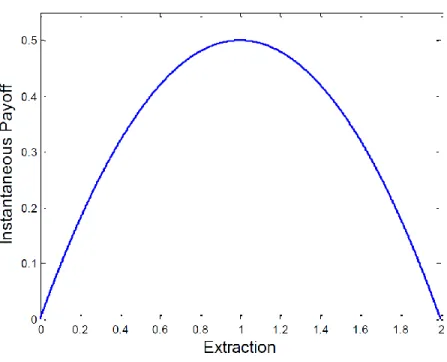
(8) Figure 1: Instant payoff function. available resource to maximize the present value of their discounted payoff over an infinite horizon. Let the extraction rate of each player i ∈ (1, 2) at time t be denoted qi (t). The evolution of the stock is given by ˙ = δS(t) − S(t). X. qi (t). with. S(0) = S0 ,. and agent i0 s payoff at time t is ui (qi (t)) = qi (t) −. qi (t)2 . 2. Note that the instantaneous payoff (depicted in Figure 1) reaches its maximum when q = 1.7 Assuming that the state variable can be observed and used for conditioning behavior, 7. If we assume two countries exploiting a common fishery ground for consumption in the domestic markets. 5.

(9) we focus on the set of stationary Markovian strategies, qi (t) = φi (S(t)).. Thus at any point in time the extraction decision of an agent depends only on the state of the stock at that moment. These strategies are simple in structure, do not require precommitment to a course of action over time and have been assumed to be a good description of realistic behaviour (Dockner and Sorger, 1996). Each agent i takes the other agent’s strategy as given and chooses a Markovian strategy that maximizes Z∞ Ji =. ui (qi (t))e−rt dt. 0. s.t. ˙ = δS(t) − qi (t) − φj (S(t)) S(t) S(0) = S0 qi (t) ≥ 0, where r > 0 is the common discount rate. We assume that δ > 2r, i.e., that the marginal productivity of the stock is high relative to the discount rate of the players. This assumption ensures existence of positive stable steady state stock levels (Dockner and Sorger, 1996, Benchekroun, 2008). In general the feedback equilibrium of a differential game is derived from the solution of the Hamilton-Jacobi-Bellman equation (Dockner at al., 2000). Let (φ∗1 , φ∗2 ) be a subgame perfect Markov Nash equilibrium. Let Vi (S) be player i0 s value function such that Vi (S) = R∞ ui (φ∗i S ∗ (t))e−rt dt with S(0) = S (Tsutsui and Mino,1990). For our problem the Hamilton0. with a linear inverse demand function Pi = 1 − q2i ; i = 1, 2 and zero marginal cost, then the instantaneous payoff function gives the instantaneous profit for each country.. 6.

(10) Jacobi equation for agent i is rVi (S) = max [qi (t) −. qi (t)2 + Vi0 (δS(t) − q1 (t) − φ∗j (S(t)))]. 2. Proposition 1: A symmetric Markov Perfect Nash equilibrium of this game is given by (φ∗ , φ∗ ) such that. φ(S) =.     0,    . for S <. 2r − 31 + 3δ       1,. (2δ−r)S , 3. for. δ−2r δ(2δ−r). δ−2r δ(2δ−r). for S >. ≤S≤. 2 δ. 2 δ. Proof: See Appendix B. The equilibrium extraction strategy described in Proposition 1 is linear in current stock for the range of stock levels between 2 , δ. δ−2r δ(2δ−r). and 2δ . Note that if the stock level is higher than. best consumption of the resource for both agents is ensured: each agent extracts at the. rate of 1, which is the rate that gives the highest instantaneous payoff.. Proposition 2 : The game admits a continuum of symmetric Markov Perfect equilibria. The inverse of an equilibrium strategy is given by S(q) =. −δ 2 3(1 − q) − + C(1 − q) −r+δ , δ 2δ − r. where C is an arbitrary constant of integration that belongs to an interval defined by the condition of stability of steady states. Proof: See Appendix B. When C = 0 we obtain the the linear increasing portion of global Markov Perfect Nash equilibrium strategy, described in Proposition 1. Each value of C < 0 above a lower bound 7.

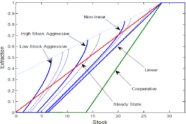
(11) gives a locally defined non-linear Markov-perfect equilibrium strategy.8 Let the steady state extraction of the resource by each player in a symmetric equilibrium be denoted by qss and the steady state stock be denoted by Sss . Corollary 1 : For the equilibrium defined in Proposition 1 we have , qss = 1 2 Sss = . δ For C < 0 above a lower bound given by the condition of stability of steady states we have r−δ 2r − δ ) 2δ−r Cδ(2δ − r) r−δ 2 2r − δ Sss = (1 − ( ) 2δ−r ). δ Cδ(2δ − r). qss = 1 − (. Proof: See Appendix B. The steady state extraction rate and stock of the resource is an increasing function of C, as C → 0, qss → 1, which gives the largest instantaneous payoff at the steady state. Thus with C < 0, the larger the absolute value of C, the more aggressive is the corresponding strategy, causing the agents to be worse off in the long run. Figure 2 presents several examples of equilibrium strategies in this game for parameter values we chose in the experiment. In the figure, the horizontal axis is the stock level and the vertical axis is the extraction rate. The strategy labelled ‘Linear’ is the non-cooperative linear strategy (i.e., C = 0). To the right of this strategy, labelled ‘Cooperative’, is the cooperative linear strategy, i.e., the strategy that maximizes the joint welfare of both players (but not an equilibrium result of the non-cooperative game).9 The line called ‘Steady State’ represents steady-state extraction at different stock levels, where q =. δS . 2. The locally defined curved. lines represent different non-linear equilibrium strategies (i.e., C 6= 0), with lower steady 8. A global Markov-perfect Nash equilibrium strategy is defined over the entire state space (Benchekroun, 2008). A local Markov-perfect Nash equilibrium strategy is defined over an interval of the state space and supports a stable steady state within that interval (Dockner and Wagener, 2013). 9 See Appendix B.. 8.

(12) Figure 2: Representative Equilibrium Strategies. 9.

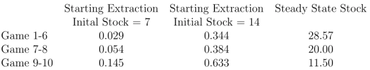
(13) state stock levels resulting as the curve representing the strategy moves left on the graph towards the vertical axis.10. 3. Experimental Design. Our experiment is a continuous time simulation of an infinite resource extraction game. In the experiments, subjects view, in real time, the dynamics of the stock level while setting their extraction rate. The experimenter sets the initial extraction rate and the starting stock level, the simulation begins, and then the subjects are free to change their extraction rates with an on-screen slider. Our parameter selection reflects the need for the simulation to be manageable while providing an empiricial test of linear vs. non-linear strategies. In order to provide a strong test of the predisposition of subjects to play different strategies, we varied our experimental design along two dimensions. First, our design consists of several games within each session with different starting extraction rates. Holding the initial stock constant but varying the subjects’ initial starting extraction rate places them on a different equilibrium path at the start of the experiment, allowing us to test whether the initial condition has an effect on the strategy played in the game. Second, our design consists of two separate treatments with different initial stock levels, while holding the strategy implied by the initial extraction constant across treatments. Increasing the initial stock level eliminates a set of equilibrium strategies that exist at the lower initial stock level, providing no theoretical reason for a behavioral effect if linear strategies dominate behavior. Table 1 summarizes the experimental design. The first two columns of the table present the starting extraction rates for initial stock levels of 7 and 14. The third column shows the predicted steady-state stock levels for the non-cooperative equilibria corresponding to the starting extraction rates (note that the steady state stock level is identical for both initial 10. See Appendix B for the time paths of stock level and extraction for different equilibrium strategies.. 10.

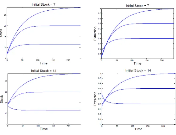
(14) Table 1: Experimental Parameters. Game 1-6 Game 7-8 Game 9-10. Starting Extraction Inital Stock = 7 0.029 0.054 0.145. Starting Extraction Initial Stock = 14 0.344 0.384 0.633. Steady State Stock 28.57 20.00 11.50. stock levels). The rows show which of the ten games contained which parameters. For games one through six subjects were placed on an initial path for the non-cooperative linear strategy (the line labelled ‘Linear’ in Figure 2), with an initial extraction rate of 0.029 and 0.344 in the two treatments. In games seven and eight, the initial extraction rate implies the non-linear strategy labelled ‘Non-linear’ in Figure 2. And in games nine and ten, the initial extraction rate implies the non-linear strategy labelled ‘High Stock Aggressive’ in Figure 2. To see this note that when the starting stock is 7 one of the most aggressive strategies available is the ‘Low Stock Aggressive’ strategy depicted in Figure 2. However, if the starting stock is 14, one of the most aggressive strategies available is the ‘High Stock Aggressive’ strategy. The higher starting stock of 14 eliminates the non-linear strategies between those two strategies. The time to reach the steady state depends on the replenishment rate δ, the discount rate r, and the initial stock level. We chose the replenishing rate δ = 0.07 and the discount rate r = 0.005 so that, for any of our initial stock levels the theoretical time to reach any steady states is a maximum of something less than four minutes. Figure 3 presents the equilibrium dynamics for both the stock level and extraction rate for each of the different experimental treatments. The graphs on the left show the dynamics of the stock level and the graphs on the right show the same information for the extraction rate. The two graphs at the top of the figure display this information for the lower starting stock level, and the two graphs at the bottom represent the higher starting stock level. Within the figures, the (top) curve represents the linear non-cooperative equilibrium, and the lower curves represent increasingly competitive non-linear equilibria. 11.

(15) Figure 3: Predicted Time Paths For Experimental Parameters. The right-hand portion of Figure 3 shows the dynamics of the extraction rates. Notice that the starting extraction rate is inversely related to the steady-state stock level. This is intuitive: low initial extraction rates allow the stock to build up at a faster rate. Notice also that for the highest starting extraction rate, when the initial stock level is 14, the theoretical extraction rate decreases over time, enhancing our ability to identify the play of non-linear strategies in the data. Looking at the dynamics of the stock levels, notice that in both treatments the final stock level is identical for each of the three initial extraction rates. For example, the steady-state stock level is approximately 28.57 in both graphs for the non-cooperative linear strategy 12.

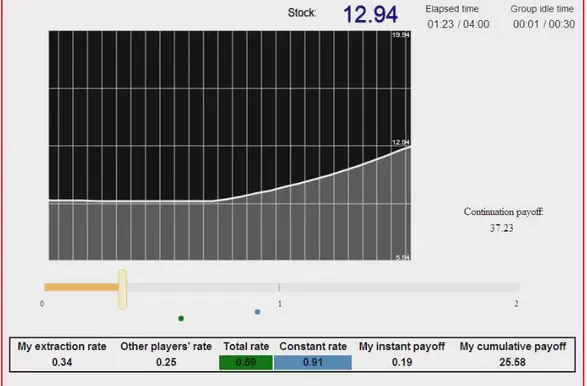
(16) equilibrium, and approximately 11.5 for the more aggressive equilibrium. The longest time to the steady state stock level occurs with the linear strategy. This is reflected by the fact that the highest steady-state stock level is reached in this case.. 4. Experimental Procedures. We implemented this real-time continuous renewable resource game in a computer laboratory.11. Subjects were presented the screen shown in Figure 4. At the top of the screen,. subjects were shown the current stock level (12.94 in the figure), the elapsed time in the game, and the amount of time idle, i.e., the time since the last subject changed her or his extraction rate. If this number ever reached 30 seconds, we assumed a steady state had been reached and stopped the simulation. We implemented the discount rate by applying it to subjects’ payoffs every second. When the simulation stopped, either after four minutes or after 30 seconds of player inactivity, the computer computed the discounted sum of payoffs for the subject out to infinity. This computation assumed that the extraction rate stayed the same forever as it was at the end of the simulation, and took into account whether the stock level would ever go to zero. On the right of the screen near the middle, the “continuation payoff” that subjects would receive if the simulation were to stop was always displayed. We presented this information to give subjects a better feel for the fact that their pay included both their actual resource extraction and what they would extract if the game went forever.12 11. As described in Brehmer (1992) decision making in real time is decision making “in context and time”. In this setting decisions are made in an “asynchronous fashion” with constant updates of information (Huberman and Glance,1993). For economic experiments in continuous time see Oprea and Friedman (2012) and Oprea, et al. (2011). Janssen, et al (2010) have also studied a common pool resource problem in real time. 12 In economics experiments there are two basic approaches to address the issues of infinite horizon and the presence of time preference. One is to impose an exogenous probability of termination of the round at any time t. The other approach is to let the decision making task last for a fixed period of time and add a justifiable continuation payoff, where the payoff during the round and after it should be discounted appropriately. Noussair and Matheny (2000) and Brown, Christopher and Schotter (2011)) show. 13.

(17) Figure 4: Experiment Screen Shot. 14.

(18) The black rectangle in the middle of the screen showed the dynamics of the stock level in a continuously sliding window. Just below, a slider could be moved left or right with the computer mouse to set the current extraction rate. Below the slider was a blue dot that informed the subjects of the total extraction rate that would hold the stock level constant. Also below the slider was a black dot that showed the total extraction rate, i.e., the sum of the two players’ extraction rates. Numbers across the bottom of the screen included the subject’s own extraction rate, the other player’s extraction rate, the total extraction rate, and the rate at which the stock level would be held constant. The instant payoff and the cumulative (discounted) payoff for the game were the final two items of information on the screen. Subjects were informed everything about the model, including the stock replenishing rate, discount rate, and the quadratic payoff function (which was a minimum at extraction rates 0 and 2 and a maximum at extraction rate 1). They were told that the structure of the game would always stay the same for every game, but the intial extraction rate, which would be identical for both subjects, might change for different games (see Appendix A for the instructions for the treatment with starting stock level equal to fourteen). Before playing the two-player games, subjects were required to pass a test that would provide common knowledge among the participants that all subjects knew how to control the stock level with their extraction rate. Specifically, all subjects were given fifteen tries, as monopolists, to manipulate the stock level from five to twelve, hold it constant for a moment, and then reduce it to seven, using their extraction rate as a tool, within one minute. Payoffs were not discussed until after subjects passed the test. Subjects who did not succeed were dismissed and paid their show up fee. In 19 experimental sessions there were 67 pairs consisting of 134 subjects earning an average of $26, including a standard $10.00 show-up fee at the CIRANO experimental labthat behaviour is not significantly different under different approaches of discounting in their laboratory experiments.. 15.

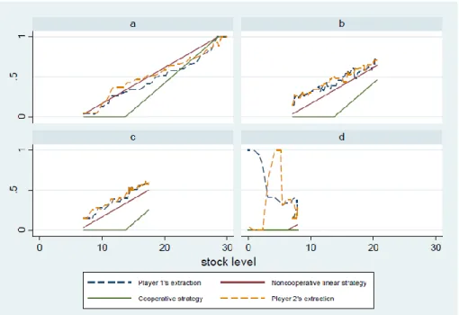
(19) oratory in Montreal. In total, thirty-three pairs of subjects played the first treatment and thirty-four pairs of subjects played the second treatment. Sessions lasted no more than two hours. Twenty-five subjects were dismissed for failing the pre-test.. 5. Experimental Results. 5.1. Extraction Types. There was a high degree of heterogeneity among the different groups (each group consists of a pair of subjects), but play can basically be characterized as resulting in an end of game stock that (1) maximizes long-term extraction rates, that (2) falls short of maximizing but is greater than zero, and that (3) is equal to zero. Figure 5 shows an example of the extraction decisions for four different subject pairs. In each of the sub-figures, the horizontal axis depicts the stock level and the vertical axis represents the extraction rate. The two dashed lines represent the extraction decisions of the two players; the green line, which indicates a zero extraction rate up to a stock level of approximately 15 shows the linear cooperative strategy, and the brown line (located above the green line) shows the linear non-cooperative strategy. Panel a in Figure 5 presents the extraction decisions of a pair that are qualitatively similar to the linear non-cooperative strategy. In Panels b and c the extraction strategies appear fairly linear but the extraction rates are higher than in Panel a. And in Panel d we present the decisions of a pair that are nothing remotely like an equilibrium strategy: this subject pair quickly ran their stock level to zero. In general, we classify three different types of groups according to the stock level they reach by the end of their play. Type 1 groups reach a stock level equal to or better than the most desirable stock level where the extraction rate for each player can attain the maximum instantaneous payoff of 1. Type 3 groups reach a stock level of zero. Type 2 groups reach a 16.

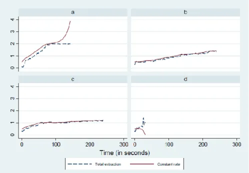
(20) stock level between Type 1 and Type 3. If these types are not apparent in Figure 5, they become more so in Figure 6, which is a plot of the same subject pairs’ total extraction rate over time. In the figure, the horizontal axis represents simulation time in seconds and the vertical axis is the sum of the two players’ extraction rates at each instant. Panels a, b, c, and d display results for the same subject pairs as the identical panels in Figure 5. Panel a reveals that this pair reached a steady state level where the sum of the players’ extraction rates in the steady state reached a maximum of 2. If we only consider the final game in all the sessions, 13 out of 33 groups in Treatment 1, and 12 out of 34 groups in Treatment 2 were Type 1 groups. Panel d shows that this particular pair reduces the stock level to zero 0. Six groups in the first treatment and 3 groups in the second treatment were Type 3 in the final game. Panels b and c show examples of extraction rates at the end of the game less than 2 but greater than 0. The remaining groups were Type 2. The behavior of the third type is analogous to the predicted behaviour of a myopic agent, with a strategy that is given by q(t) = 1. Given our initial stock levels myopic behaviour of the subjects will take the stock to 0 in finite time. See Appendix B for more on description of myopic behaviour.. 5.2. Distribution of Steady States. Every equilibrium strategy we consider supports a stable steady state of the stock and extraction. Thus we begin our analysis of the results by obtaining the distribution of steadystates in the data. First, we define a steady state and show how we identify one in choice data. Second, we present the distributions of steady states by game and by treatment. The problem of identifying the time of convergence of a process for the purpose of characterizing a steady-state is well-known in computer simulation literature, which is convenient for our application because of our need to identify the time of the theoretical steady state 17.

(21) Figure 5: Examples of Different Actual Extraction Behaviours. 18.

(22) Figure 6: Examples of Actual Total Extraction Time Paths. 19.

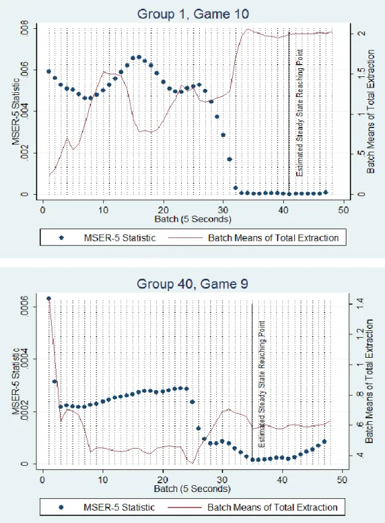
(23) Figure 7: Locating the Steady State. 20.

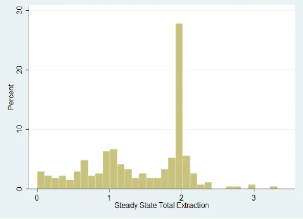
(24) both for experimental design and for comparison with subject behavior. Many computer simulations, such as Markov Chain Monte Carlo methods in Bayesian analysis, result in a “warm-up” or “burn-in” before reaching steady-state. In some cases, one can simply run the algorithm well into a point where a steady state has been obviously reached. In our case, we first must identify if a steady state exists. If so we wish to accurately and automatically identify the extraction rate. Several algorithms exist for automatic detection of a steady state. The algorithm we chose is called MSER-5 (Mean Squared Error Reduction or Marginal Standard Error Rule). We chose this method because it is automatic, easy to understand and implement, and robust for our application. Roughly, the algorithm deletes data points in steps from the beginning of a series, recursively computing the standard error of the mean or MSER statistic of the truncated sample. The truncated sample with the smallest MSER contains the data points that are at the steady state.13 Figure 7 illustrates the identification of steady states using the MSER-5 algorithm. The two panels show the time series of the total extraction rate (the sum of the two players’ extraction rates) by five second batch means, in an actual game in two different experimental sessions. The MSER-5 statistic is depcited by the dotted line, while the extraction rate is given by the solid line. In the top panel, the steady state level is identified just after 200 seconds in the game. In the bottom panel it is identified at approximately 175 seconds. Note that the algorithm does not always identify a steady state from the data. If the MSER-5 continues to fall throughout the entire series , a steady state is not reached. We found that running this procedure on all of our data results in intuitively reasonable inference as shown in Figure 7. Figure 8 presents the histogram of steady states for all the play that reached a steady state in the experiment. The figure gives a broad overview of the performance of the subject 13. For the details of MSER-5 algorithm see Appendix C.. 21.

(25) pairs. Notice the mode at a total extraction rate of two, which is jointly the most efficient (abstracting from the time path to this steady state). There appears to be another mode at one, but every possible extraction rate between zero and two appears at least two percent of the time. There are relatively few, but more than zero, steady state extraction rates above two. Overall the histogram shows a rich degree of heterogeneity of reasonable outcomes that could be the result of equilibrium strategies. Table 2 shows the percentage of player pairs that reached a steady state by treatment for every game for pay. At least 61% of the pairs reached a steady state in every game, and the mean steady state total extraction rate was at least 1.2 for every game. The table also indicates the ranges of steady-states reached in each game. We can conclude from this table that in every game in each treatment the majority of behavior resulted in steady-state stock management. Table 2: Percentage of Games Reaching a Steady State Treatment 1. Treatment 2. (So = 7). (So =14). (%). mean. range. (%). mean. range. Game 5. 70%. 1.36. 0.04-2.16. 65%. 1.48. .34-2.99. Game 6. 79%. 1.2. .02-2.06. 65%. 1.4. 0.28-3. Game 7. 64%. 1.37. 0-2.01. 71%. 1.49. 0.54-2.1. Game 8. 70%. 1.49. 0.25-2.4. 65%. 1.53. 0.31-3.3. Game 9. 61%. 1.26. 0.01-2.1. 62%. 1.6. 0.08-2.36. Game 10. 67%. 1.46. 0.05-2.37. 71%. 1.56. 0.14-2.8. Focusing on games 6, 8 and 10 (which were each the last game in a set of identical games), we conducted a Kolmogorov-Smirnov test for the difference in steady state distributions across games within treatments. For both treatments, we cannot reject the null hypothesis 22.

(26) that the distributions across the different games are identical. We then pooled across all games within each treatment to test for a difference in behavior across the treatments, where we rejected the null that the pooled distributions are identical. For a look at these distributions, Figure 9 presents a density estimate of the distribution of steady-state total extraction rates for each of our two experimental treatments. In Figure 9, the horizontal axis of the density estimate represents the steady state total extraction rate. The solid graph shows the density estimate for the initial stock of seven and the dashed graph presents the density estimate for the initial stock of fourteen. Three features are striking. First, the distribution of steady states is bimodal in both treatments. Second, the mode centred on the total extraction rate of two is nearly identical in both treatments. Third, the mode below two is shifted to the right for the treatment with the higher initial stock. Recall that raising the initial stock simply eliminated the worst set of non-linear aggressive strategies from the set of equilibrium strategies. The effect of eliminating these strategies appears to have had no effect on the groups of players who achieved the maximum stock level extraction rate, i.e. the minimally aggressive player pairs. Conversely, eliminating non-linear strategies has the effect pushing the more aggressive player pairs in the direction of, but not achieving, best steady state. Our experimental treatment thus allows us to divide player pairs according to whether they are minimally aggressive or not. Eliminating the worst aggressive equilibria does not induce minimum aggression, and has no effect on those players who are already less aggressive. This gives us a large clue as to how people play the game. Finally we conducted a test for symmetry of extraction strategies among the subject pairs. We used the heuristic of dividing the total extraction rate by two, and then determining whether both players’ extraction rates were within 10% of this number. Of the 270 games that reached steady-state, 144 were symmetric by this definition. Figure 10 shows a scatter plot with the steady state extraction rates of one of the two players on each axis. The. 23.

(27) Figure 8: Distribution of Steady States. 24.

(28) Figure 9: Distribution Steady States By Treatment. red data points along the forty-five degree line indicate the games in which both players’ extraction rates were within 10% of the mean extraction rate in the steady state. The figure shows a wide variety of asymmetric steady-state extraction rates as well as the roughly half of the symmetric games along the 45 degree line. Having obtained evidence for a variety of steady states as well as a significant amount of symmetric extraction, we now turn to the question of what strategies the players are using, and how they can help us predict the level of cooperation achieved in the game.. 5.3. Extraction Strategies. Having documented the existence and distribution of steady states in the choice data, and having found that in roughly half of the cases with steady states the extraction rates were symmetric, we now test for linearity in the extraction strategies, the central question of the paper. For the purpose of building an empirical model, recall that the non-linear equilibrium 25.

(29) Figure 10: Player 1 vs. Player 2 Steady State Extraction Rates. 26.

(30) strategies do not have an explicit functional form. However, we can approximate these strategies by a quadratic function of the stock level of the following form:. q = α + γS + θ(S)2 , where q denotes the extraction rate and S denotes the stock level of the resource. This model would be sufficient to closely describe any theoretical strategy. In fact the R-squared on simulated data is typically in the neighborhood of 0.99 for any strategy we tested. However, we would like to include variables that might influence decision-making that are not considered in our theoretical model. Reasonable candidate variables are the own lagged extraction rate, (an indicator of smoothing), the extraction rate of the other paired subject (present if one subject followed the lead of the other), and time (which would indicate a holding strategy to allow the stock level to build up). All of this leads to the following general model:. qt = β0 + β1 St + β2 (St )2 + β3 qt−1 + β4 qother,t−1 + β5 t + et where qt is the current extraction of the subject, St is the current stock level of the resource, qt−1 is the lagged extraction rate, qother,t−1 is the lagged extraction rate of the paired subject, t is the time of the extraction rate decision in seconds, and et is the error term. Ideally we would run a pooled regression on our panel data, but the distribution of steady states presented in the previous section suggests a large degree of heterogeneity that would not be captured in such a model. Thus we run subject-by-subject individual regressions for each game. Such a collection of regressions on 804 sets of individual choice data presents challenges in presenting the results. These challenges stem from at least two sources: (1) how to report coefficient estimates and (2) how to select the appropriate specific model for each individual regression.. 27.

(31) To attack the problem of model selection, we used the general to specific modelling approach, which searches for the most parsimonious restriction of the general model that conveys all of the information in the general model, and within which does not exist a nested model that also conveys this information (Hoover and Perez, 1999). We take this final model as the inferred empirical strategy of a subject in a particular game. Note that extraction rates do not go below zero, and in the theoretical model no equilibrium strategy involves an extraction rate above one (which delivers the maximum instantaneous payoff, regardless of how large the stock level becomes). We observe similar empirical lower and upper bounds in the choice data. For some subjects, we observe a lower bound in the form of a constant low initial extraction rate, held constant apparently to allow the stock level to grow. We also observe an upper bound in the form of the steady state extraction level. Therefore we run a two-limit Tobit regression, with empirical lower limits and an upper limit of one. In the data, there are 804 sets of choice data, each set consisting of a subject making extraction decisions in one of the the six game s/he plays with another subject for pay. Each game can last for up to 240 seconds. Every game contains all of the data specified in our general empirical model. Our computer algorithm for model selection for the extraction decision is detailed in Appendix C. Table 3 and 4 presents a summary of the variables that comprise the estimated extraction strategies. In Table 3, each row corresponds to a particular model. For example, the first row presents statistics for strategies that have a linear component in the state variable. The second row presents information for strategies that have a non-linear component in the state variable and the third row is for strategies that do not condition at all on the state variable, which we call rule of thumb strategies.14 Note that each row adds to 100%. The columns 14. These strategies typically take the form of little or no extraction until the stock level builds to a higher level, at which time constant extraction is used. Many variants of these exist in the data. The ideal form of such a strategy is: q(S) = 0 if 0 ≤ S < 28.57 and q(S) = 1 if S ≥ 28.57. See more on rule of thumb strategies in Appendix B.. 28.

(32) represent the subset of data analysed. For example, the first column represents treatment 1, the third column represents all of the data, and the fourth column is for data that contains a steady state. Table 3: Types of Estimated Strategies Trearment 1. Treatment 2. All. All SS. Linear in Stock. 24.74%. 30.92%. 27.89%. 25.92%. Non-linear in Stock. 59.60%. 55.86%. 57.72%. 57.04%. Rule of Thumb. 15.66%. 13.22%. 14.39%. 17.04%. ‘Linear in Stock’ implies non-zero coefficient for S and zero coefficient for S 2 in the estimated strategy. ‘Non-inear in Stock’ implies non-zero coefficient for S 2 in the estimated strategy. ‘Rule of Thumb’ implies zero coefficients for S and S 2 in the estimated strategy.. Table 4: Non-Theoretical Conditioning Variables Trearment 1. Treatment 2. All. All SS. Depends on Lag Extraction. 92.93%. 96.51%. 94.73%. 97.41%. Depends on other’s Lag Extraction. 50.25%. 49.63%. 49.94%. 48.89%. Depends on Time Elapsed. 56.31%. 52.37%. 54.33%. 52.59%. The table provides the first evidence for or against empirical equilibrium strategies. Notice that across the board, roughly one-quarter of the models selected are linear in the stock variable; over half are non-linear in the stock level; and roughly 15% are what we call rule of thumb, i.e., do not condition on the stock level at all. With regard to the two treatments, there was a slight shift into linear models and out of non-linear and rule of thumb models from treatment one to treatment two. And the largest difference in models selected between games with and without a steady state was the increase in rules of thumb in games with steady states. Subjects appear to be allowing the stock level to increase before beginning their extraction. This finding is similar to a finding in Janssen, et al. (2010). A common. 29.

(33) strategy similar to our rule of thumb strategy was discussed and implemented in their communication treatment, where the players wait without harvesting for a time span to let the resource grow. Table 4 provides a quick summary of the control variable content of the selected models. Briefly, the table confirms that there is nearly always inertia in the setting of the extraction rate, that roughly half the time extraction strategies condition on the extraction rate of the other paired subject, and that half of the strategies condition on time (for the most part, increasing extraction with time, controlling for all other explanatory variables). Table 5: Distribution of Steady States by Strategy Type Treatment 1. Treatment 2. Both. (So = 7). (So =14). Treatments. Mean. SD. obs. Mean. SD. obs. Mean. SD. obs. Linear in Stock. 1.226. 0.73. 62. 1.34. 0.67. 78. 1.29. 0.7. 140. Non-linear in Stock. 1.295. 0.71. 156. 1.52. 0.6. 148. 1.408. 0.67. 304. Rule of thumb. 1.69. 0.59. 52. 1.72. 0.54. 44. 1.7. 0.56. 96. The central result of Table 5 is the statistically significant improvement of steady state stock levels among the non-linear strategies from Treatment 1 to Treatment 2 (a KolmogorovSmirnov test rejects the null hypothesis of equality at better than 5%). By contrast, a Kolmogorov-Smirnov test fails to reject the null of equality of the steady state distributions between treatments for the estimated strategies linear in stock. Recall that higher initial stock eliminates some of the more aggressive non-linear strategies in our theoretical solution. Here we find that in Treatment 2 starting with higher initial stock improves the steady state reached by the strategies non-linear in stock. Having described the variables that are contained by the empirical strategy models, we report the average of the estimated coefficients on the state variables for estimated strategies non-linear in stock. This information is provided in Table 6, where the mean coefficient on 30.

(34) Table 6: Distribution of Coefficient Estimates for the Non-linear Strategies Treatment 1. Treatment 2. (So = 7). (So = 14). mean. SD. range. mean. SD. range. S. -0.01437. 0.2366. -2.78 - 0.638. 0.0326. 0.335. -1.43 - 1.947. S2. 0.00018. 0.0042. -0.029 - 0.035. -0.000437. 0.01176. -0.0628 - 0.58. the stock and stock-squared variables are presented for both treatments. In this table we have a result: a one tail t test shows that the mean coefficient of stock is significantly smaller in treatment 1 at the 10% level (p value = 0.0805). The central result of Table 6 builds on that of Table 5. Although we do not reject the null of equality of the mean of coefficient of stock squared between the treatments in a one tail t test, the estimated coefficient on stock increases from Treatment 1 to Treatment 2, and decreases on stock-squared. Thus both coefficients from Treatment 1 to Treatment 2 move in the direction predicted by less aggressive non-linear equilibrium strategies. The conclusion is that increasing the stock level decreases the aggressivity of the non-linear strategies employed by players in this game.. 6. Discussion. It is worthwhile to compare our experiment to the experimental literature on common pool resource problems, which have been studied mostly in discrete time with a wide variety of institutional manipulations. One such manipulation involves communication as a method to endogenously form rules for commons self-governance (Ostrom et al., 2006). Many others have been tested as well. Herr et al. (1997) and Mason and Phillips (1997) study a common pool resources game with both static and dynamic externalities. Mason and Phillips (1997) investigates the effect. 31.

(35) of industry size on harvesting behaviour. They use infinitely repeated games to show that cooperation generated by repeated interaction with small industry size helps to mitigate tragedy of the commons in the presence of static externality, but it does not help in the presence of dynamic externality. The common pool resource problem in an intergenerational setting has been studied in Fischer, et al. (2004) and Chermark and Krause (2002). Vespa (2011) studies types of strategies used to sustain cooperation in a dynamic common pool resource game in discrete time with a small discrete choice set. His study shows that Markovian strategies are well representative of behaviour in such environment. In a dynamic public good game Battaglini et al. (1012b) shows similar results and predicts that complexity of the choice set likely to increase application of Markovian strategies. Janssen et al. (2010) use an experimental environment to closely approximate the field settings to study common pool resource problems. To mimic the field the experiment include both spatial and temporal dynamics and subjects make decisions in real time. They test the role of communication and costly punishment to improve cooperation. Our experiment is different in several ways. First, in our experiment, the only dynamic externality is in terms of future availability of the resource. Second, our choice space and state space is continuous. Third, agents interact in real time. Fourth, we a have continuum of non-cooperative Markovian equilibrium strategies including one that can support the best steady state. With our basic results in hand, our experimental setting admits the types of institutional manipulations that have been tested in these other environments.. 7. Conclusions. We presented an experiment in which subject pairs harvested a renewable resource in real time. We tested this institution under two different experimental manipulations. First, we started the game along three different equilibrium paths. Second, we started the game with. 32.

(36) different initial stock levels, holding constant the initital equilibrium path. We found the former had no effect on behavior, but the latter manipulation had an effect. We found evidence for strategies with both linear and non-linear components of the state variable, as well as rule-of-thumb strategies. The fact that there is evidence for the use of nonlinear extraction strategies is important and has implications for several areas of application of differential games such as in capital accumulation games, dynamic oligopolies with sticky prices, stock public good games or shallow lake pollution games where a continuum of nonlinear equilibria were shown to exist.15 We found that play evolves over time into multiple steady states. Among the subject pairs that reach a non-zero resource level in the steady state, we found a bimodal distribution of steady states, indicating two different levels of aggressivity of resource extraction. Rule of thumb strategies involved setting a very low or a zero extraction rate to quickly increase the stock level to the point where it supports a high steady state extraction rate. When we eliminated a set of non-linear strategies, contrary to an absence of a theoretical prediction, we found increased cooperation within the more aggressive pairs coming from an improvement in the non-linear strategies they employ. Further evidence regarding the strategic weight placed on the square of the stock level led us to conclude that eliminating the worst non-linear strategies (off the path of the initial equilibrium) improved outcomes among the groups that employed non-linear strategies. On the other hand, different initial resource extraction rates, i.e., different initial equilibrium paths, had no measured effect on behavior. Our results have implications for the management of non-renewable resources. First, while many strategies resemble the form of equilibrium strategies, good outcomes were achieved with the simple technique of focusing on raising the stock level before extracting significant amounts of the resource. Our conjecture is that in the presence of competitive 15. See Kossioris, Plexousakis, Xepapadeas and de Zeeuw (2011) for the case of shallow lake pollution game.. 33.

(37) extraction, and the strategic uncertainty it creates, this rule of thumb behavior represents a safe method for managing the resource. And this method results in steady-state extraction leves similar to the (best) linear equilibrium. Second, the sensitivity of the more aggressive non-linear strategies to the initial stock level suggests that improvement in renewable resource extraction may be attained by ensuring a healthy initial resource level. Policies that ban extraction or that ban extraction on a subset of the resource, for example fish below a certain size, allowing the builiding up of the stock of the resource now have an empirical foundation as a result of our experimental findings. Our results suggest that such a policy may permanently increase the stock level through resulting improvement in extraction strategies.. 34.

(38) 35.

(39) 36.

(40) 37.

(41) 38.

(42) 39.

(43) 40.

(44) 41.

(45) Appendix B : Proofs and Derivations Non Cooperative Equilibria Proof of Proposition 1 and 2 Given the Hamilton-Jacobi-Bellman equation (HJB), associated with the problem of agent i (Dockner et al, 2000) : rVi (S) = max [qi (t) −. qi (t)2 + Vi0 (δS(t) − q1 (t) − q2 (t))] 2. (1). The F.O.C. is qi∗ =.    1 − Vi0 , if Vi0 ≤ 1 if Vi0 > 1.   0,. Note that qi = 1 if Vi0 = 0. Given the nature of our problem Vi0 < 0 is not possible as there is no cost of having too much stock. By substituting the first order condition in HJB and imposing symmetry we obtain rV (S) = (1 − V 0 ) −. (1 − V 0 )2 + V 0 (δS − 2(1 − V 0 )) 2 rV =. if. 0≤V0 ≤1. (1 − V 0 )(1 − 3V 0 ) + δSV 0 . 2. Taking the derivative with respect to S gives (r − δ)V 0 = (−2 + 3V 0 + δS)V 00 .. (2). The condition −2 + 3V 0 + δS 6= 0 is necessary for the value function to be continuously differentiable, which is needed for our solution method (Rawat, 2007). The equality −2 + 3V 0 + δS = 0 42.

(46) gives us the non-invertible locus, q=. 1 + δS . 3. (3). Now if we define p = V 0 we can write (2) as (r − δ)p = (−2 + 3p + δS). dp , ds. or ds (−2 + 3p + δS) = . dp (r − δ)p Then the family of solution is given by S(p) =. −δ 3p 2 − + Cp −r+δ , δ 2δ − r. (4). where C is the constant of integration. A solution V (S) to the Bellman equation can be implicitly described in a parametric form (1 − p)(1 − 3p) + δSp, 2 −δ 2 3p S(p) = − + Cp −r+δ . δ 2δ − r. rV (p) =. Each value of C generates a candidate value function. The corresponding candidate equilibrium strategy is given by S(q) =. −δ 2 3(1 − q) − + C(1 − q) −r+δ . δ 2δ − r. (5). We can define a subgame perfect Markov Nash equilibrium (φ∗ , φ∗ ) setting C = 0 such as φ∗ (S) =. 2r 1 (2δ − r)S − + . 3δ 3 3. 43. (6).

(47) More specifically, the equilibrium is characterized     0,     φ(S) = 2r − 1 + (2δ−r)S , 3δ 3 3       1,. by for S < for. δ−2r δ(2δ−r). δ−2r δ(2δ−r). for S >. ≤S≤. 2 δ. 2 δ. and the value function   δ−2r δ−2r   ), for S < δ(2δ−r) e−rt(S) V ( δ(2δ−r)     R∞ 2 δ−2r V (S) = (φ(S) − φ(S) )e−rt dt, for δ(2δ−r) ≤S≤ 2   0      0.5 , for S > 2δ r where, t(S) is such that. δ−2r δ(2δ−r). 2 δ. = Seδt(S) .. The following figure shows some of these candidate strategies for the range of values of C from −3 to 3 and for parameter values r = 0.005 and δ = 0.07.. 44.

(48) The red thick line is the steady state line defined by q = is the non-invertible locus, along which. dq dS. δS , 2. and the light blue thick line. = ±∞ (Rowat, 2007). The thin curves are can-. didate strategies. As the strategies left to the linear strategy intersect the non invertibile locus they cease to be functions, therefore the strategies left to the linear strategy starting from the horizontal axis up to the non invertibile locus characterized the locally defined non-linear Markov-perfect equilibrium strategies. The candidate strategies to the right of the linear strategies can be dismissed by the argument of “profitable deviation from their play” (Rowat,2007, Dockner and Wagener, 2013) . As these strategies always lie bellow the SS line stock will be ever growing, and at some point in time the the stock will reach 2δ . After this point it is always profitable to set q = 1.. Steady States A steady state level of resource is determined by S(q) =. −δ 2 3(1 − q) − + C(1 − q) δ−r δ (2δ − r). and. δS = 2q.. A steady state is therefore a solution of −δ 2 2 3(1 − q) − + C(1 − q) δ−r = q δ (2δ − r) δ. or −δ 2 3 [ − ](1 − q) + C(1 − q) δ−r = 0. δ (2δ − r). Now for C 6= 0 the steady state extraction and stock corresponding to different values of C are given by r−δ 2r − δ ) 2δ−r Cδ(2δ − r) r−δ 2 2r − δ Sss = (1 − ( ) 2δ−r ). δ Cδ(2δ − r). qss = 1 − (. 45.

(49) For C = 0 the steady state extraction rate and stock levels are given by 2 3 δ − 2r − = 6= 0 δ (2δ − r) δ(2δ − r) qss = 1 2 Sss = . δ. Stability of Steady States At the steady state stability requires dS˙ <0 dS or δ−2. dq <0 dS. or 2 dS < dq δ or −δ 3 δ 2 + C(1 − q) δ−r −1 < , 2δ − r δ − r δ. where for C 6= 0, q is given by the steady state extraction rate qss(δ, r, C) = 1 − (. r−δ 2r − δ ) 2δ−r , Cδ(2δ − r). and for C = 0 the stability of the steady state requires (given 2δ − r > 0) 3 2 < . 2δ − r δ Therefore as long as 2δ − r > 0 and δ − 2r > 0 the steady state of the linear strategy is stable. 46.

(50) Time Paths The time path of the stock and extraction rate for the linear strategy can be derived as follows ˙ = δS(t) − 2φ∗ (S) S(t) or ˙ = δS(t) − 2( 2r − 1 + (2δ − r)S ). S(t) 3δ 3 3. Therefore with ˙ = S( 2r − δ ) + 2 ( δ − 2r ) S(t) 3 3 δ. and. S(0) = S0 ,. we obtain the solution for the time path of the stock and the time path of the extraction rate when the players are using the linear symmetric Markovian equilibrium strategy δ−2r 2 2 + [So − ]e−( 3 )t δ δ 2r 1 (2δ − r)S(t) − + . q(t) = 3δ 3 3. S(t) =. To obtain an expression for the dynamics of the stock level and extraction rate for any symmetric Markovian equilibrium strategy, including the linear strategy, we proceed as fol˙ as a function of S(t), we lows. Since we cannot obtain an analytical expression for S(t) ˙ as a function of p(t) where p(t) = 1 − q(t) from instead express p(t) S(p) =. −δ 2 3p − + Cp δ−r δ (2δ − r). or r−2δ δ 3 ˙ = p(t)(C( ˙ S(t) )p(t) δ−r − ). r−δ 2δ − r. We thus have ˙ = δS(t) − 2q(t), S(t) 47.

(51) or −δ ˙ = δ( 2 − 3p(t) + Cp(t) δ−r S(t) ) − 2(1 − p(t)). δ (2δ − r). Therefore ˙ = p(t) ˙ = p(t). ˙ S(t) r−2δ. δ C( r−δ )p(t) δ−r −. δ( 2δ −. 3p(t) (2δ−r). 3 2δ−r −δ. + Cp(t) δ−r ) − 2(1 − p(t)) r−2δ. δ C( r−δ )p(t) δ−r −. 3 2δ−r. .. Now we obtain a first order non-linear differential equation which can be solved numerically for p(t) using, e.g., routines such as ode45 in MatLab. We can then recover q(t) and S(t).. Cooperative Solution In the cooperative solution the players maximize the discounted sum of their joint payoff. Z∞ M ax(Ji + Jj ) =. (ui (qi (t)) + uj (qj (t)))e−rt dt. 0. s.t. ˙ = δS(t) − qi (t) − qj (t) S(t) S(0) = S0 .. Assuming δ > r and qi (t) = qj (t) = q(t) we can derive the Markovian cooperative extraction strategy. 48.

(52) q(S) =.     0,    . for S <. 2δ−2r δ(2δ−r). r 2δ−2r − 1 + (δ − 2r )S, for δ(2δ−r) ≤S≤ δ       1, for S > 2δ .. 2 δ. The time path of the stock level and extraction rate in the cooperative solution are. 2 + (S0 − δ δ q(t) = 1 + (2 − 2. S(t) =. 2 (r−δ)t )e δ r 2 )(S0 − )e(r−δ)t . δ δ. Myopic Agent If we consider myopic agent, then q(t) = 1 which gives the state evolution as S(t) = [S(0) − 2 δt ]e δ. + 2δ . That is if we start with stock >. with stock <. 2 δ. 2 δ. the stock will explode over time. If we start. the stock will tend to 0 over time. And if it is equal to. 2 δ. it will stay there. (Rowat, 2007).. Rule of Thumb Strategy We can imagine rule of thumb strategies, that could be behaviourally relevant, where extraction behaviours can be described bu keeping a low extraction level and waiting for the stock to increase and then switching to the best extraction rate. These strategies can be described as stationary Markovian strategies which are piecewise continuous. An example of such an strategy is. q(S) =.    0, if 0 ≤ S < 28.57   1, if S ≥ 28.57. 49.

(53) Appendix C : Identifying a Steady State in the Choice Data The problem of the identification of a steady-state in the data is illustrated in Figure 11. The two panels show the time series of the total extraction rate (the sum of the two players’ extraction rates) in an actual game in two different experimental sessions. The top panel shows the total extraction rate converging to the maximium extraction rate level in just under 200 seconds. The challenge of an automated convergence algorithm is to not terminate at either of the two lower levels where the extraction rate flattened out, after 100 seconds and 150 seconds respectively. The bottom panel shows a second extraction rate time path. Notice that the extraction rate evens out between 50 and 100 seconds into the game, but then increases and flattens out again later. We would like to identify the second of these intervals as the steady-state. The problem of identifying the time of convergence of a process for the purpose of charactizing a steady-state is well-known in computer simulations. Essentially, many computer simulations, such as Markov Chain Monte Carlo methods in Bayesian analysis, begin with a “warm-up” or “burn-in” before reaching steady-state. In some cases, one can simply run the algorithm well into a point where a steady state has been obviously reached. In our case this is not possible. Several algorithms exist for automatic detection of a steady state. The algorithm we chose is called MSER-5. The algorithm works as follows. Consider the sequence Yi ; i = 1, 2, ....n with the initial condition Y0 , and where the Y ’s correspond to total extraction rate batch mean, i.e., the average of the total extraction rate in blocks of five seconds. The notational indices are in consecutive blocks of five seconds. Then the steady state mean is defined as. 50.

(54) Figure 11: Locating the Steady State. 51.

(55) µ = lim E[Yi |Y0 ]. i→∞. The MSER-5 estimates the steady state mean using the truncated sample mean. The truncated sample mean is defined as. Y¯n,d =. Pn. i=d+1. n−d. Yi. .. The time in the series at which the steady state is first identified is called the optimal truncation point. It defined as Pn. ∗. d = min [ n>d≥0. − Y¯n,d )2 ]. (n − d)2. i=d+1 (Yi. Three intuitions apply to this method. First, it minimizes the width of the marginal confidence interval of the estimate of the steady state mean (White and Robinson, 2010). Second, it has been shown that the expected value of MSER is asymptotically proportional to the mean-squared error of the estimate of the steady state mean (Pasupathy and Schmeiser, 2010). Third, the MSER truncates the stock level sequence such that the truncated mean defines the best constant regression for any truncated sequence in the sence of weighted mean squared error (White and Robinson, 2010) , thus the method is analogous to regression analysis. Intuitively, using five period block averages of the total extraction rate ensures monotonic behavior of the statistic. If the MSER-5 continues to fall throughout the entire series, a steady state was not reached. More specifically we say that a steady state is reached in a data series if the minimum MSER-5 is reached at least 10 seconds before the game ends.. The following contains some specific details on applying MSER-5 in our particular application.. 52.

(56) 1. When the stock goes to zero it is possible that the total extraction stays steady at some positive level. But this is not a steady state behaviour. Therefore we rule out all plays that ends with a zero stock level from achieving steady state. 2. The linear strategy takes the longest time to reach the steady state. When the initial stock level is 7 it takes the linear strategy 222 seconds to reach within 99% of steady state and for the initial stock level of 14 it takes 202 seconds. Therefore if the player’s strategy is close to the linear strategy, since it gradually approaches the steady state, it is possible that by 230 seconds the total extraction is still growing and our algorithm will show no steady state reached. We observe several cases like that in the data. To adjust for this we assume that the play is approaching a steady state if MSER-5 keeps falling till the end of play and the end stock is close to the linear strategy steady state (the linear strategy steady state stock is 28.57, and we say the stock is close to it if it is ≥ 28. The strategy that reaches the steady state stock level of 28 reaches 99% of the steady state stock level in 176 seconds). All the main results of of steady state analysis remain qualitatively same if we do not make this adjustment.. Appendix D : General-to-Specific algorithm Given our strategy of subject-by-subject regression analysis, we require an objective method for automatic model specification. One approach would be to simply include all the regressors in all of the models and report the distribution of point estimates that results. The approach we chose is to use a general-to-specific algorithm to present the best model from the space of all possible models for each indivdual. Since there is apparent smoothness in the extraction behaviour, a multipath search for the optimal specification of a dynamic model is required (Castle, Doornik and Hendry, 2011,. 53.

(57) Mizon,1995). Hendry and Krolzig have developed the PcGets software for just such an automated model selection. In our case, we require a two limit tobit model for our empirical strategy estimation. PcGets current version does not include automatic econometric model selection for censored models. Therefore we ran our own multipath search general-to-specific model selection algorithm according to the principle of the “Hendry” or “LSE” Methodology (Hoover and Perez, 1999, Hendry and Krolzig, 2001 and Doornik, 2009).. Our model has 5 candidate regressors giving 25 possible models to fit the data. We select one of these models according to the following multipath search algorithm:. Stage 1 : We begin by estimating the general unrestricted model (GUM). Given that we have 5 regressors in our GUM, we start five different reduction paths. Each path begins with a four regressor restricted model (RM4) dropping one of the regressors in the GUM. We continue through the path if the restricted model encompasses the GUM, i.e., if the restricted model is not rejected in favor of the GUM. We use a likelihood ratio test for the validity of the restriction for each of the five restricted models (setting our criterion for rejection at the 5% level). If none of the restricted models encompasses the GUM, we are left with the GUM as our final model for the data set.. Stage 2 : If any reduction path from stage 1 continues, that is, if any of the five restricted models encompasses the GUM, we introduce four new reduction paths. One of the four regressors from the particular RM4 from stage 1 is deleted to generate a new reduction path, where the new restricted models (RM3) are models with three regressors. If none of four the restricted models encompasses the particular RM4, we are left with that RM4 as our terminal model along that reduction path. We continue down a new path only if the particular nested RM3 encompasses its RM4. Otherwise the reduction path is terminated.. 54.

(58) Stage 3 : New reduction paths from stage 2 continue if any of the RM3 encompass the RM4. The current RM3 introduces three reduction paths in a similar manner as the earlier stages, where the new restricted models (RM2) are models with two regressors. If none of the three restricted models encompasses its associated RM3, we are left with that RM3 as our terminal model along that reduction path. Otherwise we continue through all the new reduction paths where the RM2 encompasses its RM3. If a RM2 does not encompass the RM3 the reduction path is terminated.. Stage 4 : New reduction paths from stage 3 continue if the any of the RM2 encompasses the RM3. The current RM2 introduces two reduction paths in a similar manner as the earlier stages, where the new restricted model (RM1) are models with one regressor. If none of two restricted models encompasses its RM2, we are left with that RM2 as our terminal model along that reduction path. Otherwise we have the RM1 as one of the terminal models if it encompasses the RM2 it is nested in.. Stage 5 : When we obtain multiple terminal models (most of the time non-nested), we use the minimum Akaike Information Criterion to decide on the final model.. As an example, suppose we name the regressors as 1, 2, ...., 5. The Figure 13 demonstrates a portion of the search tree. The figure shows all the reduction paths initiated from the reduction at stage 1 by dropping regressor 3. The bold green paths show two hypothetical search paths resulting in two candidate terminal models.. 55.

(59) Figure 12: Hypothetical search paths. 56.