Université de Montréal
Dynamique des communautés végétales et impacts des perturbations humaines sur la végétation des tourbières
par Salomé Pasquet
Département de Sciences biologiques Faculté des arts et des sciences
Mémoire présenté à la Faculté des études supérieures en vue de l’obtention du grade de M.Sc.
en Sciences biologiques
Avril 2014
Résumé
Ce mémoire visait à comprendre la dynamique temporelle et les patrons floristiques actuels de deux tourbières du sud-ouest du Québec (Small et Large Tea Field) et à identifier les facteurs anthropiques, environnementaux et spatiaux sous-jacents. Pour répondre aux objectifs, des inventaires floristiques anciens (1985) ont d’abord été comparés à des inventaires récents (2012) puis les patrons actuels et les facteurs sous-jacents ont été identifiés à l’aide d’analyses multi-variables. Mes résultats montrent d’abord qu’un boisement important s’est produit au cours des 30 dernières années dans les tourbières à l’étude, probablement en lien avec le drainage des terres agricoles avoisinantes, diminuant la hauteur de la nappe phréatique. Simultanément, les sphaignes ont proliférées dans le centre des sites s’expliquant par une recolonisation des secteurs ayant brûlés en 1983. D’autre part, mes analyses ont montré que les patrons floristiques actuels étaient surtout liés aux variables environnementales (pH et conductivité de l’eau, épaisseur des dépôts), bien que la variance associée aux activités humaines était aussi significative, notamment dans la tourbière Large (18.6%). Les patrons floristiques ainsi que les variables environnementales et anthropiques explicatives étaient aussi fortement structurés dans l’espace, notamment selon un gradient bordure-centre. Enfin, la diversité béta actuelle était surtout liée à la présence d’espèces non-tourbicoles ou exotiques. Globalement, cette étude a montré que les perturbations humaines passées et actuelles avaient un impact important sur la dynamique et la distribution de la végétation des tourbières Small et Large Tea Field.
Mots clés : Tourbière; Dynamique végétale; Perturbations anthropiques; Conditions
Abstract
This study aimed to understand the temporal dynamics and the current floristic patterns in two peatlands of southwestern Quebec (Small and Large Tea Field), and to identify natural and anthropogenic drivers of the changes and patterns observed. To do so, past (1985) and recent (2012) floristic surveys were compared while current floristic patterns and underlying factors were identified using multivariate analyses. Firstly, results show that tree encroachment occurred over the last 30 years, likely due to drainage of surrounding farmlands lowering the water table level. Simultaneously, Sphagnum mosses have proliferated in the center of peatlands, probably explained by the recolonization of the areas burned in 1983. On the other hand, multivariate analysis showed that current floristic patterns were mainly related to environmental variables (water pH and conductivity, peat deposits thickness), although variance associated with human activities was also significant, especially in the Large peatland (18.6%). Floristic patterns as well as explanatory environmental and anthropogenic variables were highly structured in space, following a margin-expanse gradient. Finally, the current beta diversity was mainly related to the richness of native non-peatland and exotic species. Overall, this study showed that past and current human activities had a significant impact on vegetation dynamics and distribution of the Small and Large Tea Field peatlands.
Keywords: Peatland; Vegetation dynamics; Anthropogenic disturbance; Environmental factor;
Table des matières
Résumé ... ii
Abstract ... iii
Listes des Tableaux ... vi
Listes des Figures ... vii
Liste des Annexes ... viii
Remerciements ... ix
Chapitre 1 : Introduction générale ... 1
1.1 Dynamique des communautés végétales ... 2
1.1.1 Succession végétale ... 2
1.1.2 Succession végétale dans les tourbières ... 3
1.2 Facteurs influençant la répartition de la végétation... 5
1.2.1 Facteurs environnementaux ... 5
1.2.2 Perturbations ... 7
1.2.3 Spatialité ... 9
1.2.4. Influence relative des facteurs de contrôle ... 10
1.3 Objectifs de l’étude ... 11
1.4 Organisation du mémoire ... 11
Chapitre 2: Three decades of vegetation dynamics in peatlands isolated in an agricultural landscape ... 13 2.1 Introduction ... 13 2.2 Study sites ... 15 2.3 Methods ... 20 2.3.1 Field Sampling ... 20 2.3.2 Taxonomic verification ... 22 2.3.3 Data analyses ... 22 2.4. Results ... 24
2.4.1 Floristic richness and composition changes ... 24
2.4.2 Tree encroachment and species composition and richness ... 27
2.4.3 Environmental changes ... 31
Chapitre 3: Relative influence of abiotic and anthropogenic factors on vegetation of two
peatlands. ... 37
3.1 Introduction ... 37
3.2 Methods ... 40
3.2.1 Study area and sites ... 40
3.2.2. Sampling and data collection ... 42
3.2.3 Data analysis ... 45
3.3 Results ... 47
3.3.2 Plant species assemblage ... 52
3.3.3 Species composition and relative influence of abiotic, anthropogenic and spatial factors ... 56
3.4 Discussion ... 57
Chapitre 4 : Conclusion générale ... 61
Bibliographie ... 65
Listes des Tableaux
Chapitre 2
Table 1. Plant species communities in the Large and Small Tea Field peatlands, southwestern
Québec (Canada) ... 19
Table 2. Indicator species of old forests, new forests and open habitats ... 30 Table 3. Percentage of fire disturbed area in 1984-85, mean percent cover of open surface water,
mean pH, mean ditch density and mean percent disturbed area ... 32 Chapitre 3
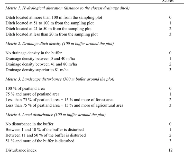
Table 1. Description of the four metrics used to calculate the disturbance index for each sampling
plot ... 44
Table 2. Environmental variables sampled in the 102 sampling plots and their abbreviation .... 47 Table 3. Mean of some explanatory variables in the Small and Large Tea Field peatlands ... 48 Table 4. Number of species sampled in Tea Field peatlands ... 48 Table 5. Multiple regression analysis between the local contribution of beta diversity and
explanatory variables in the two study peatlands ... 50
Table 6. Spearman correlation between LCBD and richness of different groups of plant species at
the Small and Large Tea Field peatlands ... 50
Table 7. Mean percent of native peatland, native non-peatland and exotic species for each plant
Listes des Figures
Chapitre 2
Figure 1. Location of the peatlands studied (southwestern Québec, Canada), and of the sampling
plots within the peatlands ... 16
Figure 2. Significant changes (Chi-square goodness-of-fit tests; p ≤ 0.05) in species’ frequency
of occurrence (number of plots) from 1984-85 to 2012 ... 26
Figure 3. Changes in species mean cover between surveys in 1984-85 and 2012 ... 27 Figure 4. Spatio-temporal evolution of the forest cover of the Large and Small Tea Field
peatlands ... 28
Figure 5. Linear Discriminant Analysis (LDA) of the three habitat categories made on species
abundance in 2012 survey ... 29
Figure 6. Mean number of peatland and non-peatland (including exotic) species in each habitat
type ... 31 Chapitre 3
Figure 1. Location of the Tea Field peatlands, southern Quebec, Canada ... 41 Figure 2. Map showing the local contribution of beta diversity for each sampling plot in the Tea
Field peatlands ... 51
Figure 3. Spatial distribution of the plant species assemblage with time-constrained clustering
according to Ward method in Tea Field peatlands ... 54
Figure 4. Canonical redundancy analysis biplot examining the strength of association among
environmental variables, the plant species assemblages and the species in Tea Field peatlands . 55
Figure 5. Venn diagrams showing the partition of the total variation explained by abiotic,
anthropogenic disturbance and spatial variables in the vegetation composition of Tea Field peatlands ... 57
Liste des Annexes
Appendix 1. Plant species found in the Small Tea Field and Large Tea Field bogs in 1984 and
2012, southwestern Quebec (Canada) ... x
Appendix 2. Code, name, number of sampling plots and classification of species sampled in Tea
Field bogs in 2012, southwestern Québec (Canada) ... xiv
Annexe 3. Coordonnées géographiques des 102 parcelles échantillonnées dans les tourbières
Small et Large Tea Field. Indice S: Small Tea Field; L: Large Tea Field ... xix
Annexe 4. Caractéristiques physico-chimiques des 102 parcelles échantillonnées dans les
tourbières Small et Large Tea Field ... xx
Annexe 5. Classes d’abondances des espèces échantillonnées dans les 102 parcelles des
Remerciements
Je voudrais tout d’abord remercier ma directrice de maitrise, Stéphanie Pellerin, pour m’avoir soutenue et encouragée tout au long de ce projet. Je la remercie également pour sa disponibilité, son optimisme constant et sa confiance en moi.
Je tiens également à remercier ma co-directrice, Monique Poulin. Bien que loin physiquement, ses suggestions et ses encouragements ont été d’une grande aide durant ces deux années.
Je remercie Martin Jean de m’avoir permis d’utiliser ses données récoltées en 1985 pour ma présente étude.
J’aimerais aussi remercier les personnes m’ayant aidé à collecter les données sur le terrain : Emmanuelle Bergeron, Karim Bouvet, Stéphanie Gervais, Jean-Sébastien Mignot et Audrey Anne Derome.
Merci également à Matthieu Charrier, Jean Faubert et Robert Gauthier, pour leur collaboration respective dans l’identification de spécimens de plantes vasculaires, de mousses et de sphaignes.
Je voudrais aussi remercier Pierre Legendre et Stéphane Daigle pour l’aide fournie dans la réalisation des analyses statistiques.
Je remercie tout particulièrement mon conjoint, ma famille et mes amis pour leur soutien continuel tout au long de mes études.
Merci également à mes collègues du laboratoire Pellerin pour les nombreuses discussions.
Je voudrais remercier aussi Conservation de la Nature pour les autorisations d’accès aux tourbières Tea Field.
En terminant, je souhaiterais remercier le Centre de la Science de la Biodiversité du Québec et le Conseil de recherche en sciences naturelles et en génie du Canada de m’avoir octroyé une aide financière.
Chapitre 1 : Introduction générale
Les zones humides, auxquelles appartiennent notamment les tourbières, les marais et les marécages, sont des milieux intermédiaires entres les milieux terrestre et aquatique, se caractérisant par une nappe phréatique proche de la surface et par une forte productivité biologique (Barnaud & Fustec 2007). Ces écosystèmes couvrent 9% de la superficie mondiale des terres (Zedler & Kercher 2005) et fournissent divers services écologiques tels que l’amélioration de la qualité de l’eau, la régularisation des débits des cours d’eau, la séquestration du carbone et le support de la biodiversité (Gorham 1991; Charman 2002; Levison et al. 2013). Cependant, 50% de la superficie mondiale des zones humides ont été perdues au cours des derniers siècles et la plupart de celles encore présentes aujourd’hui sont dégradées (Moser et al. 1996; Zedler & Kercher 2005), principalement dues à l’urbanisation, l’agriculture et la sylviculture (Moser et al. 1996). Or, la modification des composantes de ces écosystèmes, et notamment celle de leurs communautés floristiques, peut constituer une menace sérieuse au maintien de leurs fonctions écosystémiques. Par exemple, la disparition des sphaignes et leur remplacement par des espèces vasculaires souvent associées au drainage des tourbières diminuent le taux d’accumulation de la matière organique et donc celui du carbone (Moore 2001). Dans ce contexte, ce mémoire visera à comprendre les facteurs responsables du façonnement des communautés floristiques des tourbières du sud du Québec, d’abord avec une perspective temporelle et ensuite avec une perspective spatiale. Dans les pages suivantes, une revue de littérature portant sur la dynamique des communautés végétales ainsi que sur les facteurs influençant la répartition de la végétation sera d’abord présentée afin de mettre en contexte le mémoire.
1.1 Dynamique des communautés végétales
1.1.1 Succession végétale
Les communautés végétales sont définies à la fois par la richesse et l’abondance des espèces ainsi que par leurs relations écologiques. Avec le temps, et surtout des conditions environnementales changeantes, les caractéristiques de la communauté évoluent. En effet, certains organismes vont apparaître alors que d’autres vont disparaître, ce qui entraine le changement de la communauté. On parle de succession pour désigner ces enchainements temporels, cycliques ou linéaires dans les écosystèmes (Gillet et al. 1991). Chaque transformation dynamique est caractérisée par quatre critères: l’origine des éléments qu’elle met en jeu (succession primaire ou secondaire), son sens (succession progressive ou régressive), sa cause (succession autogène ou allogène), et sa nature (changement d’espèces dominantes) (Decocq 1997).
Tout d’abord, on distingue la succession primaire de la succession secondaire par le fait que le développement de communauté végétale a lieu dans des habitats nouveaux dépourvus de végétation. La succession secondaire consiste pour sa part dans le retour à la végétation après une perturbation (Ricklefs & Miller 2005). On distingue également la succession régressive, où le biotope se dégrade et la communauté diminue sa biomasse et sa biodiversité, de la succession progressive, où la communauté devient stable et augmente sa biomasse (Walker et al. 1983). La succession peut aussi découler de modifications induites par les organismes eux-mêmes, il est alors question de succession autogène. L’évolution d’un étang vers une forêt impliquerait par exemple des processus de succession autogène selon la séquence suivante: en raison de la diminution du niveau de l’eau due à l’accumulation de matière organique, les arbres et arbustes tolérants l’immersion s’installent et assèchent au fur à mesure le milieu, qui deviendra en quelque temps une forêt terrestre. Les successions peuvent également provenir de modifications induites
par des facteurs externes à la communauté (p.ex.: climat, feux, perturbations anthropiques), c’est la succession allogène. Dans la succession de l’étang vers un marais par exemple, de fortes précipitations et un mauvais drainage favoriseraient l’accumulation d’eau et ainsi la croissance d’une végétation hydrophile adaptée à ces conditions (Courchesne 2012). Ainsi, des changements graduels d’habitats et de communautés végétales se succèdent dans le temps pour atteindre un stade final le plus stable possible, appelé climax.
1.1.2 Succession végétale dans les tourbières
Dans les tourbières, la succession végétale à long terme est essentiellement liée aux variations climatiques et à des processus autogènes associés à la croissance verticale de la surface des tourbières, en lien avec l’accumulation continuelle des restes végétaux (Payette 1988). Dans les régions tempérées et boréales, le patron général de développement des tourbières s’effectue principalement en deux phases, soit une phase minérotrophe suivie d’une phase ombrotrophe. Cette succession, appelée ombrotrophication, peut se produire rapidement (entre 50 et 350 ans) ou être un phénomène graduel pouvant s’étendre sur environ 2000 ans (Kuhry et al. 1993). C’est un processus complexe pour lequel il y a encore beaucoup de débats sur les éléments déclencheurs, mais qui serait vraisemblablement associé à des changements climatiques et/ou hydrologiques et/ou au processus interne d’accumulation de la tourbe (Payette 1988; Hughes & Barber 2004; Robichaud & Bégin 2009). Par exemple, la mise en place de conditions climatiques fraîches et humides aurait induit l’ombrotrophication dans certaines tourbières (Robichaud & Bégin 2009), alors qu’elle serait plutôt associée à des périodes plus chaudes et sèches dans d’autres tourbières (Pajula 2000). L’ombrotrophication peut aussi être le résultat unique de l’accumulation progressive de la tourbe, engendrant l’élévation de la surface de la tourbière au-dessus de la nappe phréatique et permettant ainsi aux sphaignes de se développer et de devenir
l’espèce dominante du milieu (Tremblay 2013). Peu importe le processus autogène ou allogène déclenchant l’ombrotrophication, cette succession est toujours caractérisée par la mise en place d’un couvert de sphaignes. Une fois présentes dans le milieu, les sphaignes forment un environnement défavorable pour de nombreuses plantes vasculaires en créant des conditions acides, pauvres en éléments nutritifs et anoxiques, favorisant ainsi leur propre maintien (van Breemen 1995). L’ombrotrophication peut néanmoins être inhibée et même inversée par l’apport d’eaux riches en nutriments dans la tourbière (Pajula 2000; Haraguchi & Nakazono 2011). Il est alors question de minérotrophication, c’est à dire le passage d’une tourbière ombrotrophe à une tourbière minérotrophe.
Certains changements environnementaux peuvent aussi engendrer des modifications dans la flore des tourbières sans toutefois en changer le statut trophique. Par exemple, l’augmentation de la dominance des arbres dans les tourbières est généralement associée à un réchauffement climatique et à des périodes de sécheresse (p.ex.: Weltzin et al. 2000; Breeuwer et al. 2009; Keuper et al. 2011 ; Heijmans et al. 2013). En effet, des températures plus élevées vont diminuer la hauteur de la nappe phréatique, augmenter la disponibilité des nutriments et allonger la saison de croissance, cela résultant en des conditions favorables de croissance pour les arbres (Heijmans et al. 2013). Cependant, le boisement des tourbières peut également être associé au drainage ou à l’accroissement des dépositions azotées (p.ex.: Pellerin & Lavoie 2003a; Linderholm & Leine 2004; Berg et al. 2009). Bien que ce phénomène n’implique pas de changement de statut trophique, il provoque néanmoins des bouleversements dans la diversité floristique des tourbières (Woziwoda & Kopec 2014). Néanmoins, Heijmans et al. (2013) ont avancé que ce phénomène pouvait être réversible dans le temps, mais cela reste à vérifier pour les paysages plus modifiés par l’homme.
1.2 Facteurs influençant la répartition de la végétation
1.2.1 Facteurs environnementaux
Dans les tourbières de l’hémisphère nord, les variations floristiques sont principalement associées à trois gradients écologiques, soit un gradient micro-topographique (Wheeler & Proctor 2000; Okland et al. 2001; Bragazza et al. 2005), un gradient bordure-centre (Malmer 1986; Okland et al. 2001) et un gradient chimique (Wheeler & Proctor 2000; Bragazza & Gerdol 2002; Bragazza et al. 2005).
Le gradient micro-topographique, principalement régi par la hauteur de la nappe phréatique, explique la répartition des espèces en fonction de la topographie de surface des tourbières. Il existe en effet une grande différence d’humidité entre les buttes (hummocks) et les dépressions (hollows) puisque la nappe phréatique ne suit pas la microtopographie de surface des tourbières (Andrus et al. 1983; Gignac 1992). La profondeur de la nappe phréatique, contrôlant alors le degré d’humidité de la tourbe affecte la ségrégation des espèces le long de ce gradient en lien
avec la capacité des sphaignes à tolérer la dessiccation et à la capacité des plantes vasculaires à
tolérer des conditions anoxiques (Bragazza & Gerdol 1996; Henkin et al. 2011). Ainsi, Okland (1990) a trouvé une relation très forte entre la distribution de la végétation et la hauteur moyenne de la nappe phréatique dans 800 parcelles d’une tourbière boréale. La profondeur de la nappe phréatique influence également le pH et la concentration en éléments nutritifs, ceux-ci étant plus élevés dans les dépressions que dans les buttes.
La distribution des espèces vasculaires dans les tourbières, notamment celle des arbres et des arbustes est en partie régie par le gradient bordure-centre (Okland et al. 2001). Les facteurs associés à ce gradient sont multiples et varient généralement d’un site à l’autre (Wheeler & Proctor 2000; Bragazza et al. 2005). Néanmoins, la fluctuation annuelle de la hauteur de la nappe
phréatique, plus grande en bordure qu’au centre de la tourbière, et une meilleure aération de la tourbe en bordure favorisant la croissance des arbres sont les deux facteurs les plus souvent cités (Bragazza et al. 2005). Les arbres, notamment présents en bordure réduisent alors le rayonnement accessible aux autres plantes et augmentent la litière au sol, ce qui est susceptibles de modifier la végétation en favorisant les espèces forestières (Okland et al. 2001). Le long du gradient bordure-centre, deux gradients secondaires importants quant à la ségrégation des espèces, notamment des bryophytes, peuvent également être observés: un gradient d’épaisseur de tourbe et d’ombre (Jeglum & He 1995; Whitehouse & Bayley 2005). En effet, l’épaisseur de tourbe ainsi que la luminosité sont significativement plus élevées dans les zones ouvertes présentes au centre des tourbières que dans les zones boisées de bordure où les espèces forestières remplacent les espèces tourbicoles (Whitehouse & Bayley 2005). Enfin, le gradient bordure-centre serait aussi associé au fait que les bordures sont souvent plus riches que le centre puisqu’elles reçoivent une eau riche en minéraux en raison de la proximité du sol minéral (Ingram 1967; Damman & Dowhan 1981). Ainsi, les espèces indicatrices de minérotrophie sont généralement plus abondantes en bordure qu’au centre de la tourbière (Sjors 1950; Damman & Dowhan 1981; Malmer 1986; Asada et al. 2003; Pellerin et al. 2009).
Finalement, le gradient chimique permet d’expliquer la répartition de la végétation entre les tourbières ombrotrophes (pauvres) et les tourbières minérotrophes (riches). Bien que ce gradient s’exprime à l’échelle régionale (entre les tourbières), il peut aussi s’observer à l’intérieur d’une même tourbière (Sjörs 1948; Tahvanainen et al. 2002). Ce gradient est étroitement lié au pH et à la conductivité (Andersen et al. 2011a) et suggèrent une séparation graduelle entre la végétation ombrotrophe et la végétation minérotrophe (Okland et al. 2001). Ainsi, les zones ombrotrophes dominées par les sphaignes et les éricacées ont un pH et une alcalinité plus faibles (pH < 5.5 et conductivité corrigée < 80 µS/cm2) que les zones minérotrophes, généralement caractérisées par
les mousses brunes et les carex (Andersen et al. 2011a). Ce gradient est aussi associé à un gradient d’approvisionnement en éléments nutritifs (Bridgham et al. 1996). Par exemple, l’azote, le phosphore et le potassium sont présents en très petite quantité dans les tourbières ombrotrophes puisque le recyclage des éléments minéraux est ralenti par une faible décomposition des végétaux. Ainsi, uniquement les espèces adaptées pour survivre à une très faible disponibilité en éléments nutritifs (espèces ombrotrophes) peuvent survivre (Proctor 1995).
1.2.2 Perturbations
Les perturbations, qu’elles soient d’origine naturelle (feu, vent, épidémie d’insecte, etc.) ou d’origine anthropique (drainage, coupe forestière, urbanisation, etc.) peuvent aussi jouer un rôle prédominant dans la dynamique végétale des tourbières. Dans les zones perturbées, certaines espèces s’adapteront, tandis que d’autres apparaitront ou disparaitront, ce qui pourra provoquer un changement dans les communautés végétales. Dans les tourbières, la principale perturbation naturelle est le feu, tandis que les principales perturbations anthropiques sont le drainage, la coupe forestière, l’extraction de la tourbe, la pollution atmosphérique et les feux (Moore 2002; Pellerin & Lavoie 2003a; Poulin et al. 2004).
Les études portant sur le feu montrent que cette perturbation a habituellement peu de répercussions à long terme sur les communautés végétales des tourbières ombrotrophes. En effet, bien que les feux soient particulièrement dommageables pour les arbres (Chambers 1997), la flore d’origine se rétablit généralement en quelques décennies (Kuhry 1994; Robichaud 2000; Lavoie et al. 2001; Benscoter 2006; Magnan et al. 2012). Cela est souvent dû au fait que les feux dans les tourbières n’affectent généralement que les couches superficielles de tourbe en raison du fort niveau d’humidité (Magnan et al. 2012). Ainsi, la microtopographie du sol peut revenir à son état d’avant feu grâce à la régénération, les buttes peuvent devenir des dépressions dû à la
combustion, ou bien les dépressions peuvent devenir des buttes par succession (Benscoter et al. 2005). Paradoxalement, les feux peuvent aussi avoir un impact positif sur les fonctions des tourbières (p.ex.: séquestration du carbone) en permettant aux tourbières forestières de retourner à un stade moins arboré, favorisant ainsi la croissance des sphaignes (Chambers 1997). En effet, suite au feu, la mousse Polytrichum strictum s’installe grâce à la remise en circulation des nutriments et colonise rapidement le milieu. Cette espèce, capable de tolérer un stress abiotique, va modifier l’environnement et faciliter la colonisation des sphaignes, qui deviendront par la suite l’espèce dominante (Groeneveld 2002; Benscoter et al. 2005).
À l’échelle mondiale, les activités humaines ont généralement un impact négatif sur les fonctions écologiques des tourbières (Moore 2002). Par exemple, le drainage peut avoir des effets désastreux sur le fonctionnement de la tourbière, car il peut affecter de manière permanente l’hydrologie du sol (Laine et al. 1995). Il a aussi été montré qu’à une distance inférieure à 60 m, un fossé de drainage a un impact sur le niveau de la nappe phréatique suffisamment important pour augmenter la croissance des arbres (Roy et al. 2000). Le drainage favorise ainsi l’abondance des arbres et des espèces tolérantes à l’ombre et diminue le recouvrement des sphaignes (Laine et al. 1995; Poulin et al. 1999; Frankl & Schmeidl 2000; Linderholm & Leine 2004; Pellerin et al. 2008). L’évolution de la tourbière vers une végétation forestière peut alors diminuer la diversité régionale, même si la diversité en espèces à chacun des sites est peu affectée (Laine et al. 1995). L’exploitation forestière modifie également les conditions hydrologiques mais cette fois-ci en augmentant la hauteur de la nappe phréatique et en réduisant la hauteur des buttes à cause de la compaction et de l’abrasion. Cela a alors pour effet d’augmenter l’abondance des arbustes intolérants à l’ombre, des herbacées et des sphaignes (Roy et al. 2000; Locky & Bayley 2007). Par ailleurs, les tourbières sont aussi sensibles à la pollution atmosphérique. Par exemple, une augmentation d’azote induit des changements importants dans la flore des tourbières, telle qu’une
diminution du couvert de mousses et une augmentation du couvert des plantes vasculaires (Gunnarsson et al. 2002; Heijmans et al. 2002; Wiedermann et al. 2007; Sheppard et al. 2014). En effet, les espèces non vasculaires n’ont pas de cuticule permettant l’absorption des éléments nutritifs sur toute leur surface, ce qui les rend vulnérables lorsque leur niveau d’azote arrive à saturation (Bates 2002). L’azote en surplus va alors s’infiltrer dans l’eau et le sol, devenant ainsi accessible aux racines des plantes vasculaires, qui vont ensuite pouvoir dominer le milieu (Bubier et al. 2007).
1.2.3 Spatialité
La plupart des phénomènes écologiques sont structurés par des forces ayant des composantes spatiales. La distribution des espèces résulte d’une action combinée de forces externes (conditions environnementales, perturbations) et de forces internes (dynamique de la population). Or, ces deux types de forces génèrent une configuration spatiale dans la répartition des espèces ou des communautés (Legendre & Legendre 2012). Ainsi, deux sites proches géographiquement ont plus de chance d’avoir une végétation qui se ressemble que deux sites éloignés. Par exemple, plusieurs études ont montré qu’une partie importante de la variation de la végétation des tourbières était spatialement structurée (Tousignant et al. 2010; Andersen et al. 2011b). Alors que Tousignant et al. (2010) ont montré qu’il s’agissait du fait que les variables abiotiques étaient également structurées dans l’espace, Andersen et al. (2011b) ont constaté que cela était directement relié à la distribution de la végétation. En effet, les patrons spatiaux apparaitraient grâce aux espèces abondantes, couvrant de grandes superficies et ayant une distribution agrégée. En revanche, les espèces ayant un faible recouvrement ou étant peu fréquentes ne seraient pas susceptibles de contribuer à la répartition spatiale (Andersen et al. 2011b).
1.2.4. Influence relative des facteurs de contrôle
Un des grands défis des écologistes est de déterminer l’influence relative des facteurs qui régissent les patrons de végétation (facteurs abiotique, de perturbation et spatial). Pour cela, deux méthodes peuvent être utilisées: l’étude de l’évolution de la végétation ou bien l’étude de la végétation actuelle.
Tout d’abord, plusieurs études ont utilisé des techniques paléoécologiques ou historiques pour comprendre les facteurs responsables de la dynamique végétale (Lavoie & Richard 2000; Gunnarsson et al. 2002; Pellerin & Lavoie 2003a; Pellerin et al. 2008; Kapfer et al. 2011). Par exemple, dans une tourbière du sud de la Suède, Kapfer et al. (2011) ont ainsi constaté que le nombre total d’espèces présentes dans cette tourbière était resté constant durant 50 ans mais que la fréquence des espèces avait changé significativement en réponse à des changements environnementaux tels que la température, le pH, l’humidité du sol, la disponibilité en nutriments et en lumière. Par ailleurs, Pellerin et al. (2008) ont conclu que les changements des communautés végétales survenus durant trois décennies dans deux tourbières du Québec étaient dus à l’action conjointe des activités humaines et d’une période de sècheresse. Pour leur part, Pellerin et Lavoie (2003a) ont suggéré qu’une interaction entre un climat sec, du drainage et des périodes de feux semblaient être les principaux facteurs responsables de la succession végétale contemporaine survenue dans plusieurs tourbières ombrotrophes.
À l’inverse, peu d’études ont tenté de quantifier l’influence relative des facteurs régissant les patrons de végétation en utilisant les communautés végétales actuelles. Dans une tourbière tempérée, les variables environnementales (notamment la distance à la bordure et la hauteur de la nappe phréatique) expliquent 30% de la variation de la composition floristique (Pellerin et al. 2009). De même, Tousignant et al. (2010) ont estimé que les conditions abiotiques avaient une influence prédominante sur la composition en espèces des tourbières de Lanoraie. Cependant,
bien que les perturbations anthropiques des tourbières de Lanoraie expliquaient une faible fraction de la variation de la végétation (8.2%) comparée aux variables abiotiques (25.2%), l’analyse multivariée montrait que ces deux facteurs étaient liés à la distribution de certaines plantes, notamment celle des arbres et des arbustes. Toutefois, il est a prendre en considération que les activité humaines auraient tendance à modifier les conditions environnementales plutôt que d’avoir un impact direct sur les communauté végétales (Girard et al. 2002).
1.3 Objectifs de l’étude
L’objectif général de cette étude est de comprendre les facteurs responsables du façonnement des communautés végétales de deux tourbières du sud du Québec soumises à de fortes pressions anthropiques. L’étude se fera tout d’abord avec une approche temporelle et ensuite grâce à une perspective spatiale.
Les objectifs spécifiques du mémoire sont de :
1) Reconstituer la dynamique récente (30 ans) des communautés végétales.
2) Identifier les principales perturbations naturelles et anthropiques présentes sur les sites et explorer leur influence potentielle sur cette dynamique.
3) Analyser l’importance relative des conditions environnementales, des perturbations anthropiques et des composantes spatiales sur la distribution de la végétation actuelle. Les résultats obtenus permettront d’évaluer l’impact des différentes perturbations sur les communautés végétales des tourbières et de proposer des avenues pour protéger à long terme cet écosystème.
1.4 Organisation du mémoire
Le corps du mémoire est constitué de quatre chapitres dont deux rédigés sous forme d’articles scientifiques. Le second chapitre présente la dynamique temporelle récente des communautés
végétales de tourbières soumises à des pressions anthropiques. Le troisième chapitre présente l’importance relative des facteurs qui ont conduit à la végétation actuelle des tourbières. Enfin, le quatrième chapitre présente une conclusion générale au mémoire.
Le chapitre 2 a été soumis pour publication dans Applied Vegetation Science tandis que le chapitre 3 sera soumis ultérieurement pour publication. Les auteurs sont, en ordre, Salomé Pasquet, Stéphanie Pellerin et Monique Poulin. Le premier auteur a effectué l’échantillonnage sur le terrain, le traitement et l’analyse des données, ainsi que la rédaction du présent mémoire. Stéphanie Pellerin a élaboré et supervisé le projet de recherche, ainsi que corrigé et commenté les manuscrits. Monique Poulin a également corrigé et commenté les manuscrits.
Chapitre 2: Three decades of vegetation dynamics in peatlands isolated in an agricultural landscape
2.1 Introduction
Although peatlands cover extensive areas at boreal and temperate latitudes, they are threatened locally in inhabited regions by human activities such as peat extraction, tree plantation, agriculture and urban sprawl (Poulin et al. 2004; Lindholm & Heikkilä 2012). However, the wide array of functions and ecosystem services they provide should favor social acceptance of their conservation. For instance, owing to their plant accumulation processes, peatlands contain around 30% of global soil carbon stock (Gorham 1991). They also constitute fresh water reserves and help regulate regional hydrologic fluxes (Levison et al. 2013). Furthermore, they support specialized flora adapted to harsh prevailing conditions, notably acidic and water logged soils. In temperate regions, their flora contrasts sharply with surrounding environments and contributes to increased regional diversity (Ingerpuu et al. 2001). The maintenance of the above functions and services are nevertheless at risk when peatland plant communities are altered. With intensification of the human footprint on ecosystems, it becomes crucial to increase our understanding of the factors that regulate floral composition and structure in peatlands.
Ecological factors driving vegetation patterns in pristine peatlands have been investigated in several studies since the 1950s (e.g., Sjörs 1950; Malmer 1986; Belland & Vitt 1995; Bragazza et al. 2005). Results have established that floristic variation in peatlands is mainly controlled by three ecological gradients: acidity–alkalinity, availability of nutrients and water table depth. A margin-expanse gradient is also frequently described, even though the ecological factors underlying it are complex and vary from site to site (Wheeler & Proctor 2001; Bragazza et al. 2005). Locally, secondary gradients such as peat thickness or shading are also important,
especially for bryophytes (e.g., Jeglum & He 1995; Whitehouse & Bayley 2005). More recently, some studies have shown that anthropogenic forces that directly or indirectly impact peatlands may override these natural gradients and drive peatland floristic patterns and dynamics (e.g., Feléchoux et al. 2000; Pellerin & Lavoie 2003a; Toursignant et al. 2010).
The main anthropogenic disturbance in peatlands is drainage, which usually enhances shrub and tree encroachment, hampers Sphagnum growth and facilitates the establishment of generalist or non-peatland species (Laine et al. 1995; Minkkinen et al. 1999). Some studies have also shown that climate warming (Weltzin et al. 2000; Breeuwer et al. 2009) and nitrogen input from atmospheric pollution (Berendse et al. 2001; Gunnarsson et al. 2004) may have adverse impacts on peatland vegetation, mostly on Sphagnum species. Knowledge about the impact of such anthropogenic disturbances has mostly been gained through observational studies (comparing disturbed with undisturbed sites) or short-term experiments (< 10 years). Although these studies have provided important clues regarding expected changes, they have generally been unable to capture the long-term trends of community succession that follow environmental changes. Nevertheless, some studies have met this challenge by using historical vegetation surveys conducted 30-80 years ago as baselines from which to make explicit predictions concerning temporal change that can then be tested using contemporary surveys (e.g., Backéus 1972; Gunnarsson et al. 2002; Pellerin et al. 2008; Hájková et al. 2012).
It is recognized that re-visiting permanently marked plots for studying vegetation changes lead to accurate assessments. In contrast, the use of legacy data from historical surveys with imprecise locations is challenging and can lead to biased estimation of changes. Nonetheless, it is now accepted that such studies can provide valid results, especially when inferences are based on average changes observed across sample plots, rather than on changes within individual plots (Vellend et al. 2013; Chytrý et al. 2014). In this regard, Kapfer et al. (2011) reported
compositional changes over 50 years in a Sphagnum-dominated peatland by referring to species’ optimum value for different environmental gradients. They showed an increase in frequency of occurrence of species with low indicator values for light and moisture and a high indicator value for nutrients. These changes were related to an increase in air temperature and atmospheric nitrogen supply. Similarly, a study by Pellerin et al. (2008) based on unmarked plots showed significant changes in plant composition, mainly an increase of shrub and tree cover, in two southern boreal bogs over a 32-year period. For the present study, vegetation surveys carried out in 1984-85 in two peatlands located in a landscape highly transformed by humans, were used as a baseline. We specifically aimed to (1) determine changes in plant composition between the initial survey in 1984-85 and our 2012 study, (2) identify disturbances located on and surrounding the sites and explore their potential impact on the vegetation changes, and (3) analyse the impact of recent tree encroachment on peatland flora. We hypothesized that drainage is the dominant driver of the vegetation changes, and predicted an increase of non-peatland and exotic species richness at the cost of typical peatland species.
2.2 Study sites
The Small and the Large Tea Field peatlands are located in southwestern Québec, Canada (Figure 1). They are isolated in an agricultural landscape occupied mainly by maize and dairy farms and large garden markets on organic soils. Both sites rest on rich marine clay deposits of the Champlain Sea at an altitude of 50 m at sea level. Their mean peat thickness is 267 cm (Stdev: 11 cm; min: 10 cm; max: 519 cm; Pasquet unpublished data). The mean annual temperature (1965-2012) at the nearest meteorological station (10 km) is about 6 °C and mean annual precipitation is 990 mm, 16% of which falls as snow (Environment Canada 2013). Average readings registered for both climatic variables were lower during the 10-year period
prior to the first sampling (1974-84; 6.5 °C, 968 mm) than in the 10-year period preceding our resampling (2002-12; 7.6 °C, 1073 mm). Wet nitrogen depositions have only been monitored since 1988 in the area (NAtChem 2013). The Tea Field peatlands are located in a region with some of the highest levels of wet N deposition in eastern North America (Turunen et al. 2004), with an average of 0.7 g N m-2 year-1 between 1988 and 2005 (most recent data available).
Figure 1. Location of the peatlands studied (southwestern Québec, Canada), and of the sampling
plots within the peatlands. Plots are differentiated according to their membership in the plant communities defined in 1984-85 (See Table 1 for the name of each community, B = bog, F = fen and M = marsh). Sampling stations indicated by an X were not sampled in 2012 as they were located in areas that have been lost to agriculture. STF: Small Tea Field; LTF: Large Tea Field.
Since the beginning of European settlement in the region (early 19th century), about 70% of these peatlands’ original area has been lost, mainly to agriculture. According to the historical study of Jean and Bouchard (1987), in 1863, the two peatlands were still connected, and occupied an area of 5075 ha. Fifty years later (1912), they had been disconnected and covered a total area of 3828 ha. Large areas at the margins of the bogs were already drained and cultivated (Anrep 1917). In 1936, the total area of the bogs was estimated at about 3000 ha (McKibbin & Stobbe 1936), and around 40% of their surface was in culture or in pasture while drainage ditches were
all over the place. McKibbin and Stobbe (1936) also indicated that frequent fires, mostly human ignited, has greatly reduced the thickness of peat layers in several areas. The last known fire occurred in 1983 in the Large Tea Field (Jean & Bouchard 1987). In 1984, at the time of the first vegetation inventory, the total area of the two peatlands was estimated at 1600 ha. Agriculture was again the main cause of the lost. By 2012, it had been reduced to 1115 ha, representing a further loss of 485 ha (S. Pasquet, unpubl. data). Historic human activities not only reduced the surface of the two bogs, they also had major impacts on their plant communities. Macrofossil and pollen analyzes carried out in these two peatlands (Laframboise 1987) showed that the pre-colonial vegetation was very different from the current vegetation, particularly due to the expansion of agriculture (drainage, clearing, pasture) and repeated fires. For instance, spruce nearly disappeared from the peatland (no spruce were found in 1984-85 and only one spruce sapling was found in 2012), while this species used to be abundant on the two bogs according to Anrep (1917) and McKibbin and Stobbe (1936). Using notary deeds, Bouchard et al. (1989) demonstrated that spruces were selectively lumbered in the region between 1849 and 1957. However, since 2009, 820 ha have been set aside as a conservation preserve by Nature Conservancy-Québec.
Although the area of the Tea Field peatlands has shrunk dramatically since colonization, few human activities have taken place directly in the remaining portion of the peatlands. Some tree cutting is underway at their margins, and a large all-terrain vehicle track intersects the Large Tea Field. Man-made drainage ditches (between one and three meters) also run through the peatlands, especially in the southern part of the Large Tea Field and in the central section of the Small Tea Field (Figure 1). The main ditch in the latter is intersected by seven beaver dams, however, and is thus likely ineffective for drainage. Finally, a human-ignited fire in 1983 affected most of the
the Small Tea Field.
The Tea Field peatlands are characterized by a mosaic of ombrotrophic (bog) and minerotrophic (fen) plant communities with some patches of marshes. In 1984-85, Jean & Bouchard (1987) distinguished sixteen plant communities (Table 1; Figure 1). Six bog communities (B1–B6; Table 1) were identified, mainly in the central portion of both peatlands (Figure 1). Eight fen communities (F1–F8) were also identified (Table 1), mostly at the margins of both sites (Figure 1). Finally, two marsh communities (M1-M2) were found in the Small Tea Field, mainly near beaver dams. Three of the 16 communities identified in 1984-85 (F6–F8) were entirely situated in areas that have since been lost to agriculture.
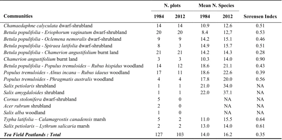
Table 1. Plant species communities in the Large and Small Tea Field peatlands, southwestern Québec (Canada). The number of plots
(N. plots) and the mean number of species per plot (Mean N. species) in each community in 1984-85 and 2012 are also indicated, as well as the Sørensen dissimilarity index. NA: not analysed
N. plots Mean N. Species
Code Communities 1984 2012 1984 2012 Sørensen Index
B1 Chamaedaphne calyculata dwarf-shrubland 14 14 10.9 12.6 0.51
B2 Betula populifolia - Eriophorum vaginatum dwarf-shrubland 20 20 8.4 12,7 0.53 B3 Betula populifolia - Oclemena nemoralis dwarf-shrubland 9 9 14.2 15.1 0.46
B4 Betula populifolia - Spiraea latifolia dwarf-shrubland 8 3 14.9 15.7 0.51
B5 Betula populifolia - Chamerion angustifolium burnt land 21 21 14.2 14.3 0.28
B6 Chamerion angustifolium burnt land 3 3 10.3 14.0 0.90
F1 Betula populifolia - Populus tremuloides – Rubus hispidus woodland 14 12 18.6 21.1 0.43 F2 Populus tremuloides - Alnus incana – Rubus idaeus woodland 17 11 18.6 22.6 0.39
F3 Populus tremuloides - Phragmatis australis woodland 4 4 17.8 20.0 0.56
F4 Salix petiolaris shrubland 1 1 21.0 34.0 NA
F5 Salix amygdaloides shrubland 1 1 22.0 37.1 NA
F6 Cornus stolonifera dwarf-shrubland 5 0 NA NA
F7 Acer rubrum shrubland 2 0 NA NA
F8 Salix alba woodland 1 0 NA NA
M1 Typha latifolia – Calamagrostis canadensis marsh 5 2 11.0 15.5 0.64
M2 Salix petiolaris – Lythrum salicaria marsh 2 2 13.0 14.0 0.61
2.3 Methods
2.3.1 Field Sampling
The vegetation of the two peatlands was first surveyed using 127 sampling plots (5 × 5 m) during the summers of 1984 and 1985 (Jean & Bouchard 1987). Most of the plots were located every 200 m along north-south transects spaced 500 m apart (Figure 1). Three supplemental plots were set up to capture smaller plant communities, while the plots in the southwestern part of the Large Tea Field were established randomly (Figure 1). Each sampling plot was set up in a homogeneous portion of the plant community. The percent cover of each plant species in each plot was estimated according to seven classes: (1) <1%, (2) 1-5%, (3) 6-10%, (4) 11-25%, (5) 26-50%, (6) 51-75%, (7) >75%. The total percent cover of burned surface and open surface water was estimated visually by projecting their horizontal coverage on the 5 x 5 m plot. The pH of the peat deposit was measured from a sample extracted ten cm below the soil surface. Samples were kept frozen in the lab until analysis. The soil pH was measured both years using a dilute Calcium Chloride (CaCl2) solution.
In 1984-85, Jean and Bouchard (1987) noted the precise position of all but four plots on a map, along with the limits of the 16 vegetation communities. In our study, we digitized, registered in space and integrated this map in Quantum GIS 1.7.4 software (QGIS), then retrieved the geographic coordinates of each plot. During the summer of 2012, we revisited 103 of the 127 sampling plots. The 24 remaining plots were either not located on the map (the four mentioned above) or were located in sectors lost to agriculture (Figure 1). In addition to geographical coordinates, we used all reported information available (e.g., position in relation to drainage ditches or roads) to determine the location of the plots. Considering the abundance of human benchmarks in the studied area, we estimated that the 2012 plots were located within 50 m
of the original plots. This sampling error should have had only a minor impact on the trends in change over time in the vegetation of these sites (Pellerin et al. 2008). All plots were sampled using the same methods as in 1984-85.
Woody plant encroachment
To assess woody plant encroachment in the two bogs, we used grey-scale aerial photographs from 1983 and 1999 (1: 15 000) as well as Google Earth’s Digital Globe satellite imagery from 2010. Aerial photographs were selected based on cloud free conditions and absence of distortion. The 1983 photos were digitized and registered in space using QGIS to be comparable with the 2010 satellite imagery. In QGIS, woody areas were manually delineated on each 1983 aerial photo and 2010 satellite image based on color and texture. Woody areas were those with more than 35% coverage of tall tree (> 2 m). Automatic methods, such as thresholding, were not suitable due to high variability in the background color of the photos. Visual interpretation of vegetation structure was, however, confirmed by stereoscopic viewing of 1983 and 1999 aerial photographs (the 1999 photos were the most recent available).
Mapping of anthropogenic disturbances
All anthropogenic disturbances located within or bordering the Tea Field peatlands were identified using georeferenced aerial photographs and satellite images. Then the perimeters of each disturbed surfaces (agricultural land, tree cutting areas, roads, all-terrain vehicle trail, drainage ditches) were delineated in QGIS. The percentage of disturbed surfaces and ditch density (m/ha) within a radius of 100 m from each sampling plot was then calculated. The efficiency of a drainage ditch in a peatland depends on several factors (e.g., peat composition and structure, ditch depth and direction), but its impact on vegetation is rarely apparent at distances exceeding 100 m (e.g., Poulin et al. 1999; Roy et al. 2000).
2.3.2 Taxonomic verification
We carefully verified plant lists, standardized all species nomenclature to conform to VasCan (Brouillet 2012), bryophytes to Faubert (2012) and lichens to PLANTS database (USDA & NRCS 2013) and corrected any past misidentification using herbarium specimens (Marie-Victorin Herbarium). When no herbarium specimen was available, we changed identification when there was clear evidence of error, for instance, when a species does not occur (historically or presently) in the study area (e.g., Aronia pyrifolia instead of A. melanocarpa). We grouped all species from taxonomically difficult groups at the genus level (e.g., Brachythecium, Carex,
Rubus, Salix, Sphagnum), as they were usually not well distinguished in 1984-85. Likewise, we
grouped all subspecies at the species level, because subspecies were rarely identified in 1984-85. For lichens, we retained only the four most common species (Cladina mitis, C. rangiferina,
Cladonia cristatella, C. multiformis), which accounted for > 90% of total lichen cover and were
easy to identify in the field. All vascular taxa were then classified as native peatland, native non-peatland or exotic species, using information in Dubé et al. (2011) and Lavoie et al. (2012).
2.3.3 Data analyses
Data in the 1984-85 study were only available at the community level and included: (1) a list of species, (2) the number of plots in which each species occurred, (3) the mean number of species per plot, (4) the mean cover of each species, (5) the mean peat pH, and (6) the covers of burned and open water surfaces. Prior to analyses, each plot sampled in 2012 was assigned to one of the 1984-85 plant communities using the 1984-85 map. In subsequent analyses, we omitted all data from communities situated entirely in sectors that had been transformed into agricultural fields (F6–F8) or with a single sampling plot in 2012 (F4, F5).
community from 1984-85 to 2012, we calculated the Sørenen dissimilarity index (Kolef et al. 2003), using the list of species from both years. We also identified the species with the greatest changes in frequency of occurrence between 1984-85 and 2012, by comparing the proportion of plots occupied by each species in each sampling period. For this comparison, we used only species occurring in at least 5 plots in both years or in a least 10 plots in one of the years for a total of 65 species analysed. Significant changes in frequency of occurrence were determined using Chi-square goodness-of-fit tests.
Species with significant cover changes were identified at the community level because, as mentioned above, the 1984-85 dataset reported only the mean cover value for each species, leaving the variance unknown. Therefore, a one-sample t-test with 95% degree of confidence was used to test whether the 1984-85 mean (treated as a constant) was included in 2012 confidence interval. Species cover was evaluated using the mid-point of each class for each community in both periods. For these analyses, only communities with at least 5 sampling plots in 2012 and species with more than 10% of mean cover in a specific community in at least one of the sampling periods were used. A similar method was used to identify changes in mean peat pH, mean open water cover and percentage of disturbed surfaces and ditch density within a radius of 100 m from each sampling plot.
Finally, using only the 2012 data, we analyzed the impact of tree encroachment on the flora of the peatlands. We first sorted the 2012 plots into three classes of habitats: (1) plots that were already forested in 1984-85 (old forest), (2) plots that became forested between 1983 and 2010 (new forest) and (3) plots that had never been forested in the time span of the study (open site). To evaluate whether the three habitat types could be segregated on the basis of plant species composition, we performed a linear discriminant analysis (LDA) using cover data of all vascular
each habitat group were then identified by the IndVal method (Dufrêne & Legendre 1997). Lastly, the number of peatland and non-peatland vascular species (including exotic species) per habitat was compared with the help of repeated-measures ANOVA. The repeated aspect of the ANOVA was necessary because the richness of one habitat group was not independent of the richness of the other. Richness of species was evaluated using all vascular species found in 2012 (224 species; Appendix S1, supporting information). Assumptions of normality and homogeneity of variances were met. Post-hoc multiple comparisons were performed using Tuckey HSD in JMP 10.0.0 (SAS Institute, Cary, North Carolina, USA). Univariate statistical analyses and multivariate analyses were performed in version 2.15.1 of the R environment (R Core Team, Vienna, Austria).
2.4. Results
2.4.1 Floristic richness and composition changes
In the eleven plant communities studied, a total of 190 taxa (159 vascular and 31 nonvascular) were sampled in 1984-85 (114 plots), and 177 taxa (150 vascular and 27 nonvascular) in 2012 (101 plots) (Appendix 1). Considering the smaller number of plots sampled in 2012, the overall richness per unit area appears to have increased, an inference in part supported by the higher mean number of species per plot in all communities (Table 1). Regardless of richness trend, there was a 35% floristic dissimilarity between 1984-85 and 2012 (Table 1); 70 species were observed only in 1984-85 and 57 species only in 2012. Most lost and new species were herbs (63 and 65% respectively). Although most were rare (≤ 5 plots) and occupied small surfaces (mean cover ≤ 10%), three lost species (Typha angustifolia, T. latifolia, Epilobium ciliatum subsp.
glandulosum) and four newly found ones (Phalaris arundinacea, Ilex verticillata, Gaylussacia
communities in which they occurred. In both studies, the vascular flora was primarily composed of non-peatland species (65% of the flora in 1984-85 and 63% in 2012; including exotic species), and the proportion of exotic species remained low (< 10%) (Appendix 1). At the community level, the floristic dissimilarity between the two sampling periods ranged from 28 to 90% (Table 1). Species turnover was particularly high in the two marsh communities (M1, M2), as well as in the Chamerion angustifolium burnt land (B6), but these communities were also represented by the fewest number of plots that could induce pseudo-turnover due to reduced sampling.
Among the 65 species tested for changes in frequency, 21 showed a significant increase (Figure 2), including two exotic species (Phragmites australis, Rhamnus cathartica), several non-vascular species (e.g., Sphagnum spp., Aulacomnium palustre, Pleurozium schreberi) and ericaceous shrubs typical of peatlands (Kalmia angustifolia, Rhododendron canadense,
Vaccinium spp. Gaylussacia baccata). In contrast, nine species were found to have decreased
significantly in frequency (Figure 2), in particular, Chamerion angustifolium. Most of the species occurring less frequently today than in 1984-85 were non-peatland herbaceous species.
Figure 2. Significant changes (Chi-square goodness-of-fit tests; p ≤ 0.05) in species’ frequency
of occurrence (number of plots) from 1984-85 to 2012. Changes in frequencies were calculated by subtracting the frequencies in 1984-85 from frequencies in 2012. On the left side are species with lower frequency in 2012 than in 1984-85, and on the right side, species with higher frequency in 2012 than in 1984-85. Only species occurring in at least 5 plots in both years or in at least 10 plots in one of the years were considered (65 species).
Mean plant cover changes
The mean cover of 11 taxa differed significantly between 1984-85 and 2012, and in either one or several of the six communities with more than five sampling plots (Figure 3). Seven of these species were peatland species (e.g., Vaccinium spp., Sphagnum spp., Oclemena nemoralis), and four were non-peatland species (Chamerion angustifolium, Rubus spp., Pteridium aquilinum,
Populus tremuloides). All species with a greater mean cover in 2012 than in 1984-85 were
peatland species occurring in ombrotrophic communities. In contrast, four of the eight species with a lower mean cover in 2012 were non-peatland species found in minerotrophic communities. The mean cover of Sphagnum spp. increased significantly in the four ombrotrophic communities, and even tripled in one of these (see B1, Figure 3). The trajectory of Betula populifolia’s mean cover between the two time periods diverged among communities, being two times higher in two bog communities and three times lower in a fen community.
Figure 3. Changes in species mean cover between surveys in 1984-85 and 2012. Only species
with significant mean cover change are presented, and this, for each community analysed. See Table 1 for the name of each community. Underlined indicates native peatland species.
2.4.2 Tree encroachment and species composition and richness
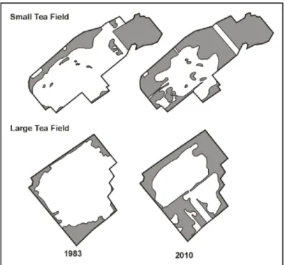
Analyses of aerial photographs and satellite images indicated that widespread forest expansion occurred in both peatlands (Figure 4). During the period studied, the percentage of the area occupied by forest increased from 26 to 51%, which represents an overall gain of 280 ha of forest habitat (Table 1). Tree encroachment was particularly noticeable at the margins of the sites (Figure 4). Betula populifolia (observed in 82% of the plots in 2012), Populus tremuloides (37%) and Acer rubrum (31%) accounted for most of the increase in forest cover.
Figure 4. Spatio-temporal evolution of the forest cover (grey sector) of the Small and Large Tea
Field peatlands, reconstructed using aerial photographs (1983 and 1999) and satellite imagery (2010).
The LDA correctly classified 97% of the sampling sites in the appropriate group: 100%, 94% and 98% of old forest, new forest and open habitats respectively. Open habitats and old forests were the most distinct groups (Figure 5). Twenty-three species were found to be indicators of old forests, one of new forests and 17 of open habitats (Table 2). All indicator species of new forest and open habitats were peatland species, while most of the indicator species of old forests (15 species) were non-peatland or exotic species (Phragmites australis, Rhamnus cathartica). Although not exotic, three invasive vines in southern Québec (Clematis virginiana,
Pathenocissus inserta, Vitis riparia) were also indicators of old forests (Table 2). Plots located in
old forests had significantly more non-peatland species than peatland species (Figure 6). In contrast, we found two times more peatland than non peatland species in new forest and 15 times more in open habitats.
Figure 5. Linear Discriminant Analysis (LDA) of the three habitat categories made on species
abundance in 2012 survey. Old forests are those that were already present in 1984-85 and new forests are those that developed between 1984-85 and 2012. Open habitats are peatland area that remained treeless. LDA correctly classified 100% of the old forest plots, 94% of the new forest plots and 98% of the open habitat plots.
Table 2. Indicator species of old forests, new forests and open habitats. Old
forests are those that were already present in 1984-85 and new forests are those that developed between 1984-85 and 2012. Open habitats are peatland areas that remained treeless. Indicator value (IV) is also shown. Only species with p-value < 0.05 are presented. † indicates non-peatland species.
Species IV IV
Old forests
Acer rubrum 0.43 Maianthemum canadense 0.23
Alnus incana subsp. rugosa 0.33 Onoclea sensibilis 0.42 Brachythecium rutabulum† 0.13 Parthenocissus inserta† 0.39 Brachythecium salebrosum† 0.15 Populus tremuloides† 0.26 Callicladium haldanianum 0.14 Rhamnus cathartica† 0.39
Clematis virginiana† 0.48 Rubus idaeus† 0.51
Cornus stolonifera 0.37 Rubus hispidus† 0.30
Doellingeria umbellata† 0.14 Rubus pubescens 0.33 Dryopteris carthusiana 0.22 Solidago gigantea† 0.34 Fraxinus pennsylvanica† 0.25 Solidago rugosa† 0.18
Impatiens capensis† 0.17 Vitis riparia† 0.40
Lythrum salicaria† 0.15
New forests
Betula populifolia 0.37
Open habitats
Aulacomnium palustre 0.26 Polytrichum strictum 0.67 Chamaedaphne calyculata 0.38 Rhododendron canadense 0.54 Cladina rangiferina 0.26 Sphagnum capillifolium 0.64 Cladonia cristatella 0.26 Sphagnum magellanicum 0.19 Eriophorum vaginatum subsp. spissum 0.46 Sphagnum papillosum 0.32 Kalmia angustifolia 0.57 Sphagnum rubellum 0.53 Ilex mucronata 0.39 Vaccinium angustifolium 0.48 Oclemena nemoralis 0.15 Vaccinium corymbosum 0.33
Figure 6. Mean number of peatland and non-peatland (including exotic) species in each habitat
type (ANOVA habitat*species: F = 56.77, P <0.0001). Bars indicate standard deviation. Different letters indicate a significant difference at α = 0.05 within each habitat type as determined by a Tukey’s test.
2.4.3 Environmental changes
The 1983 fire affected more than 50% of the surface of 6 out of the 11 communities studied (Table 3). The percentage of fire-disturbed area was particularly high (between 44 to 88%) in ombrotrophic dwarf shrublands (B1 to B6) and in the Typha latifolia – Calamagrostis canadensis marsh (Table 3). In 1984-85, the mean cover of open surface water was low (less than 5%) in most of the communities, but very high (87.5%) in the two marsh communities (Table 3). In 2012, we found no area of open surface water in any of the sampling plots, even upon revisiting the site during a wetter period (May 2013). In 1984-85, the mean peat surface pH ranged from 2.9 to 5.9, and from 2.7 to 5.2 in 2012 (Table 3). It was significantly lower in 2012 than in 1984-85 in four ombrotrophic communities (B1, B4–B6), one minerotrophic community (F3) and one marsh (M2). No significant difference was found in ditch density within a radius of 100 m from a sampling plot (Table 3). The proportion of disturbed area within a radius of 100 m from a sampling plot was significantly higher in 2012 than in 1984-85 over the entire peatland area as
Table 3. Percentage of fire disturbed area in 1984-85 (Fire), mean percent cover of open surface water (OW), mean pH
(pH), mean ditch density (DD, m/ha) and mean percent disturbed area (PD). 84 = 1984-85 data; 12 = 2012 data; CI95 % = Confidence intervals. Bold indicates significant changes. See Table 1 for the name of each community.
Fire OW84 OW12 pH84 pH12 (CI95 %) DD84 (CI95 %) DD12 (CI95 %) PD84 (CI95 %) PD12 (CI95 %)
Peatlands 10 (6-14) 17 (11-23) 2 (1-3) 6 (4-8) B1 52.5 0.5 0 2.9 2.7 (2.7-2.8) 2 (0-7) 2 (0-7) 0 (0-0) 0 (0-0) B2 61.9 0.5 0 2.9 3.0 (2.8-3.2) 15 (4-26) 35 (8-52) 1 (0-1) 7 (3-11) B3 87.5 1.3 0 3.2 3.2 (2.8-3.5) 7 (0-20) 7 (0-20) 0 (0-1) 1 (0-2) B4 44.0 5.1 0 3.2 3.0 (2.9-3.1) 0 (0-0) 0 (0-0) 0 (0-0) 0 (0-0) B5 81.6 0.5 0 3.2 2.8 (2.7-2.9) 4 (0-11) 18 (5-32) 0 (0-1) 8 (2-15) B6 87.5 1.3 0 3.3 2.8 (2.6-2.9) 36 (1-71) 36 (1-71) 2 (1-2) 6 (4-8) F1 23.9 0.5 0 3.6 3.5 (2.9-4.0) 12 (0-28) 12 (0-28) 6 (2-11) 12 (7-16) F2 0.5 0.7 0 4.5 4.5 (3.9-5.1) 4 (0-13) 4 (0-13) 4 (0-9) 4 (0-9) F3 0.5 3.0 0 5.9 5.2 (4.8-5.5) 13 (0-39) 13 (0-39) 3 (0-7) 3 (0-7) M1 52.7 68.5 0 4.4 4.8 (3.2-6.4) 53 (48-57) 53 (48-57) 3 (3-3) 12 (0-25) M2 0.5 87.5 0 5.6 5.1 (4.9-5.2) 31 (0-91) 31 (0-91) 2 (0-6) 2 (0-6)