Evaluation of Grounding Resistance and Inversion
Method to Estimate Soil Electrical Grounding
Parameters
F. H. Slaoui, F. ErchiquiUnité d’enseignement et de recherche en sciences appliquées, Université du Québec en Abitibi-Témiscamingue, 455, Boul. de
l’Université, Rouyn-Noranda, Québec, Canada, J9X 5E4 e-mail: fouad.slaoui-hasnaoui@uqat.ca
e-mail: fouad.erchiqui@uqat.ca ABSTRACT
Soil resistivity plays a key role in designing grounding systems for high-voltage transmission lines and substations. The objectives of this paper are to determine the best estimated value of the apparent resistivity or electrode grounding resistance of N-layer soil and to use a new inversion method to precisely determine earth parameters. The inversion of electrical sounding data does not yield a unique solution, and a single model to interpret the observations is sought. This paper presents a new inversion method to statistically estimate soil parameters from Schlumberger and Wenner measurements. To validate the method and test the inversion scheme, four soundings were selected: two theoretical and two in the field. The procedure was applied using test data and a satisfactory soil model was obtained.
Index Terms: electrical grounding parameters, N-layer soil, apparent resistivity, resistivity measurement interpretation
I. INTRODUCTION
Ground electrode resistance plays an important role in designing power substations and transmission towers. Predicting this resistance is very complicated in some situations, especially when the soil is represented by an N-layer horizontal model with different resistivities.
Soil conductivity can vary across seasons and the depth of each layer is usually unknown, which makes determining the grounding resistance of an electrode particularly difficult.
The N-layer soil model is a realistic representation of the actual soil. Soil parameters can be estimated based on a set of soil resistivity measurements.
Several authors have contributed to solving the problem of soil parameter estimation to achieve the best fit between measured and computed resistivity values.
The Soil Measurements Interpretation Program (SOMIP) developed by Meliopoulos and Papalexopoulos [1] statistically estimates soil parameters based on resistivity measurements, but applied to field tests using four pin or three pin measurements. The program is designed to reject erroneous measurements resulting from instrument inaccuracies and changes in local soil resistivities.
Dawalibi and Barbeito [2] used imaging methods to compute the resistivity of multilayer soils by subdividing the soil into layers with thicknesses equal to a multiple of a base value.
The authors also used a method based on convolution and multiple filter theories to examine soil resistivity measurements in multilayer soil.
Takahashi and Kawase [3] developed a very compact formula to analyze changes in calculated apparent resistivity in multilayer soils, using a comparison of ρ-a curves. However, they did not provide an analytical solution to the problem of parameter estimation in such soils.
Del Alamo [4] compared eight different techniques to develop an optimum estimation of electrical grounding parameters for a two-layered soil model.
Lagacé et al. [5] used combined electrostatic images to evaluate N-layer soil resistivities and interpret sounding measurements from Wenner and Schlumberger electrode configurations.
Slaoui et al. [6] applied linear electric filter theory to derive the resistivity transform and proposed a method to estimate N-layer soil parameters from Schlumberger measurements using a ridge regression estimator.
Slaoui et al. [7] developed an innovative method to calculate the apparent resistivity of horizontally multilayered soils using an inversion method to determine the electrical grounding parameters of N-layered earth (resistivities and thicknesses).
Lagace and Vuong [8] proposed a method with a graphical user interface to estimate soil parameters of multilayered horizontal soil. The N-layer soil model illustrated in Figure 1 is a simplification of the actual soil.
This paper attempts to better estimate soil parameters from resistivity measurements. A statistical method to estimate the parameters of an N-layer soil model from Schlumberger measurements is presented.
This interpretation method works well for field data. Two field cases are presented. The two-sounding method was selected, not because the analysis was easy using the ridge regression method, but because the interpretation was very difficult using any method.
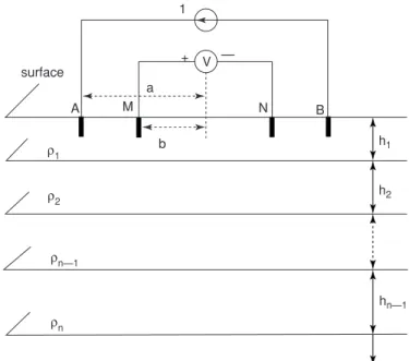
Figure 1 N-layer earth model with Schlumberger configuration.
V b a A ρ1 ρ2 ρn—1 ρn surface M 1 h1 h2 hn—1 B N + —
II. APPARENT RESISTIVITY EXPRESSIONS
Resistivity data is conventionally expressed in terms of horizontal layers having an isotropic resistivity. A model consisting of n layers would be parameterized by a set of layer resistivities ρ1, ρ2, ..., ρn, and thicknesses h1, h2, ..., hn − 1. The nth layer is the deepest and extends to infinite depth. Reducing Slaoui’s [7] calculation of theoretical apparent resistivity curves, the following general recurrence expression is obtained: (j = n − 1, n − 2, ..., 2, 1). USING SCHLUMBERGER’S ARRANGEMENT
(1)
(2) (3)
(4)
where
ρjis the resistivity of the jth layer, hj is the thickness of the jth layer,
ρjaSis the Schlumberger apparent resistivity at the jth layer, n is the number of layers in the soil model,
a is half the distance between current electrodes, and b is half the distance between voltage electrodes.
The apparent resistivity ρaSof the N-layer model is obtained at j = 1.
III. INVERSION METHOD WITH RIDGE REGRESSION
The problem of Schlumberger sounding over a plane-layered earth is nonlinear in the unknown parameters, namely, the resistivity and thickness of each layer.
As a starting point, we have a series i (i = 1, 2,..., N) of resistivity measurements ρmS, and N is the number of measurements.
In order to estimate soil parameters in multilayer soils from resistivity measurements, the least squares fitting error between the measured values must be minimized and apparent values must be analytically computed for the same spacing.
The objective function to minimize is
(5)
LEVENBERG-MARQUARDT METHOD
The Levenberg-Marquardt method is used to minimize multivariate functions. In N-layer soil, the values X = (ρ1, ρ2, ... ρn, h1, h2, ... hn−1)Tmust be determined in order to minimize the
distance function F. The F gradient is equal to zero at the absolute minimum. The Levenberg-Marquardt method consists of iteratively computing the F gradient by adjusting X from the Jacobien J such that it reduces the values of the gradient:
F=∑ − = (ρiaS ρimS) 2 i 1 N U a b b = 2− 2 G a b h i U h i a b h i a b ( , , , ) ( ) ( ) ( ) ( ) j j j = + − − + + 1 2 1 2 2 2 2 22 ρnaS=ρn kj= − + + + ρ ρ ρ ρ (j 1 aS) j (j 1) aS j ρjas( , )a b = ρj + k G a b h i, , = ∞
∑
1 ji ( , ) i 1 jFrom [4, 9], the gradient of F can be evaluated at X +∆X: (6) where (7) (8) (9) where J is a Jacobien matrix with partial derivatives of weighted differences with respect to each parameter. The apparent resistivity can be extended in the vicinity of X:
(10) Equation (10) represents a linear system of N equations with M unknowns, where the number of unknowns is 2n − 1. Since this is a nonlinear problem, by substituting (10) in (6), the application of the least-squares inverse method yields
(11) The method begins by calculating the eigenvalues of the matrix JTJ. Small eigenvalues
indicate a near-singular system, which is unstable in the presence of noisy data, and the average difference between estimated ∆X and true ∆X becomes very large. The ridge regression method [9,11] seeks to reduce this difference during the iteration process by damping the diagonal terms of (JTJ).
The ridge regression estimate of ∆Xrris
(12) where I is the unit identity matrix and .
In the above equation, α = 0 and ∆X approaches the Taylor series direction. The eigenvalues of (JTJ + αI)−1are (λ
i
2+ α), whereas λ i
2are the eigenvalues of JTJ. Increasing
the size of all eigenvalues results in significant decreases in a) the mean of the squared length between ∆X and ∆Xrrand b) the variance of the estimated solution. Therefore, in some cases, the solution ∆Xrris much closer to ∆X than the standard least-squares solution. The residual sum of squares for the ridge regression solution is given by
(13) where ∆ρ* = ρaS− ρmSis using the values X* = X + ∆Xrr.
IV. DATA ERROR AND WEIGHTING
Generally, field curves contain noise due to measuring errors, superficial inhomogeneities, telluric noise, and limited instrumentation precision.
When data are weighted, a relative degree of importance is assigned to each value. Such weighting may be used to remove inherent bias in the data or to bias the least squares fit so that it is more accurate in one area of the curve than another.
If there is a large numerical difference between the data values in different regions of the curve, an undesirable bias may be introduced into the final solution. The bias is such as to
∆S=∑ − = ∆ ∆ = ∗ ∗ (ρiaS ρimS) ( ρ ) ρ 2 i 1 N T α ≥ 0 ∆Xrr J JT I 1JT X aS mS = + − − ( α) (ρ ( ) ρ ) ∆X J JT JT X aS mS =( )−1 (ρ ( )−ρ ) J J XT ∆ +JT(ρaS( )X −ρ ) 0mS = ρaS(X+∆X)=ρaS( )X +J X∆ J X i N j n i, j iaS j 1,..., and 1,..., (2 1) =∂ ∂ = = − ρ ρmS ρ1mS ρ2mS ρNmS T , ,..., = ( )
ρaS ρ ρ1aS 2aS ρNaS
T , ,..., = ( ) ∇F X( +∆X)=2JT( (X+∆X)−∆ ) aS mS ρ
cause the ridge regression estimator to be biased toward the large values while neglecting the smaller values, which may be as accurate and may contain some very important information.
In general, it is desirable to weight each data point according to the noise in that data point, and so as not to give it a false degree of importance due to its large or small value compared with other data points.
We assume that each data point has the same percentage standard deviation unless it is known or suspected that certain points are significantly noisier. It is further assumed, initially, that each point has a standard deviation equal to one percent of its measured value. The problem standard deviation σ is then adjusted to the estimated noise level of the survey. Most resistivity surveys yield data that is accurate within five per cent or less.
The solution consists of incorporating the weights within the residual sum of squares for the ridge regression, as given by
(14) The residual error is now defined as
(15) If the error in each measurement is independent of the error in other measurements, as is usually assumed, then W reduces to a diagonal matrix of data variance σi2:
(16) The choice of a weighting scheme does not appreciably affect minimization speed. However, it can drastically affect the position of the minimum in parameter space and the parameter statistics.
The weighted ridge regression estimator is given as
(17)
V. PARAMETER STATISTICS
The next most important requirement is to obtain some idea about parameter uncertainty. The statistical parameters for our models are a) parameter standard errors and b) the parameter correlation coefficient. In addition to these statistical parameters, the parameter and data eigenvectors with the associated eigenvalues can yield great insight into the relations between individual model parameters and specific data.
Parameter standard errors and correlations are derived from the covariance matrix cov(X) evaluated at the minimum, as shown in [1, 11]:
(18)
where (19)
When is greater than σ2, σ2has been underestimated. Although the value of σ2varies
between surveys, it is assumed that the error at any data point is five percent or less. If is found to be smaller than that of the weighting, either the estimated variance of the observations have been overestimated or the curve calculated from the hypothesized model fits the noise in the data.
σ2 σ2 σ2 ρ ρ = − − ∆ T 1∆ W N M cov( )X = σ2(J W JT −1 )−1 ∆Xrr= J W JT −1 + I−1J WT −1∆ ( α ) ρ Wij i 2 0 i j i j = = ≠ σ ϕ= ρ− T −1 ρ− (∆ J∆Χ) W (∆ J∆Χ) ∆S= − ∑ = ρ ρ σ iaS imS i 2 i 1 N
Thus, the residual variance can be used as an indicator of goodness-of-fit. The residual variance is independent of the linearity or nonlinearity of the problem with respect to the model parameters.
The parameter standard errors are defined by the square root of the diagonal term of cov(X) (e.g., [cov(X)ii]1/2equals the standard error for numbered parameter i).
The correlation matrix is an indicator of the linear dependence between parameters. The correlation matrix elements are given in [2, 11].
(20) If the value of [cor(X)]ijis near unity, then the parameters Xiand Xjare strongly correlated and nearly linearly dependent. For example, if i represents the thickness h and j, the resistivity ρ of a layer (i.e., [cor(X)]ijrepresents the correlation between the thickness and resistivity of a layer), only the ratio h/ρ is well determined by the data if [cor(X)]ij = 1. This is true for layers that are highly conductive relative to their surroundings. If [cor(X)]ij= −1, only the product hρ is well determined, as is the case for relatively resistive layers. This is the familiar equivalence problem, as discussed by Sunde [10].
The diagonal elements of the covariance matrix are the variance terms for each parameter. If the correlations are small, then the standard deviation is a good measure of the uncertainty of each parameter. If two parameters are strongly correlated, then the standard deviation given by the square roots of the diagonal terms of (18) will be larger than the actual uncertainties.
The eigenvectors and their associated eigenvalues are also very useful in defining the relations between soil parameters and their effects on data generated from a particular model. The generalized inverse of J is defined in terms of these eigenvectors and eigenvalues, as described by Sunde [10].
(21) The matrix C consists of r (r is a rank of J) eigenvectors Ciof length N associated with the columns (data) of J. B comprises the r eigenvectors Biof length M associated with the rows (parameters) of J. The matrix A−1is the inverse of the diagonal matrix comprised of the eigenvalues of J.
VI. EXAMPLES OF DATA INTERPRETATION
In this section, four Schlumberger sounding curves and their associated models illustrate the ridge regression method and the estimation method for all parameter statistics.
A. THEORETICAL EXAMPLES
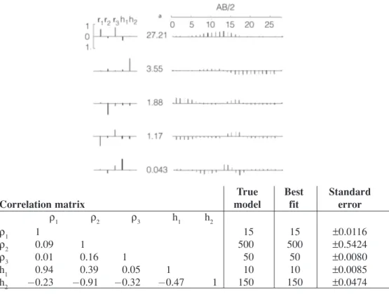
Consider theoretical model #1: X=(15, 500, 50, 10, 150), with a resistive middle layer. In Figure 2, the first column shows the eigenvectors (columns of B), the second column shows the eigenvalues (diagonal elements of A), and the third column shows the data eigenvectors (columns of C), where the abscissas represents the number of measurements. The correlation coefficients and the model parameter values with estimated standard errors, calculated using data errors as weights in equation (14), are also shown.
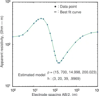
The solid curve in Figure 3 is the final fit to the data points, which appears to be very good because there is little data noise. The final estimated model is close to the original model.
The first three eigenvalues have high magnitude. The linear combination of parameters represented by the first three eigenvectors has the greatest effect on the sounding curve. In
J−1= BA C−1 T [ ( )] [cov ] [cov ] [cov cor X X X X ij ij ii 1/2 ( ) ( ) ( ) = ]]jj1/2
these three eigenvectors, the elements ρ1 and h1have opposite signs, whereas the elements ρ2 and h2have the same sign. This indicates that if ρ2and h2are both changed in the same direction, the effect on the sounding curve (Figure 3) will be larger than the effect of similar
Figure 2 Parameters and data eigenvectors with associated eigenvalues, parameter correlations, and best fit model parameters for minimization with standard error weighted data.
Figure 3 Theoretical data and best fit curve for three-layer resistivity model #1 with Schlumberger configuration.
100 101 102 103 104 105
103
: Data point : Best fit curve
102
101
Electrode Spacing, AB/2, (m) Estimated modelρ : (15,500,50)
h : (10,150)
Apparent resistivity, (0hm
−
m)
True Best Standard
Correlation matrix model fit error
ρ1 ρ2 ρ3 h1 h2 ρ1 1 15 15 ±0.0116 ρ2 0.09 1 500 500 ±0.5424 ρ3 0.01 0.16 1 50 50 ±0.0080 h1 0.94 0.39 0.05 1 10 10 ±0.0085 h2 −0.23 −0.91 −0.32 −0.47 1 150 150 ±0.0474
changes on other parameters. In addition, if ρ1 increases while h1decreases, or vice versa, the sounding curve will change accordingly.
The eigenvector associated with λ4= 1.17 indicates that increasing or decreasing ρ1 and h1together will have little effect on the sounding curve (Figure 3). In other words, the ratio h1/ρ1is the combination of these parameters that affects the sounding curve the most (note that the correlation coefficient between ρ1and h1is +0.94). The eigenvector associated with λ5= 0.043 indicates that increasing ρ2while decreasing h2, or vice versa, has little effect on
the sounding curve. Again, this is also indicated by considering the correlation coefficient between ρ2 and h2, which is −0.91.
Considering the parameter eigenvector and parameter correlation coefficients of this model, it can be seen that the products ρ2h2are better determined by, and have greater effect on, this data than either ρ2 or h2separately.
From the analysis of the eigenvectors, we see a wide range of resistivities and thicknesses for a very resistive layer that will yield nearly identical sounding curves as long as the thickness-resistivity ratio changes only slightly. In addition, for a very conductive layer, there is large range of resistivities and thicknesses that yield nearly the same sounding curve as long as the resistivity-thickness product is relatively constant. Thus, the parameters of highly resistive or highly conductive layers are difficult to determine. The correlation matrix must be considered in any interpretation of the standard deviations given by equation (18).
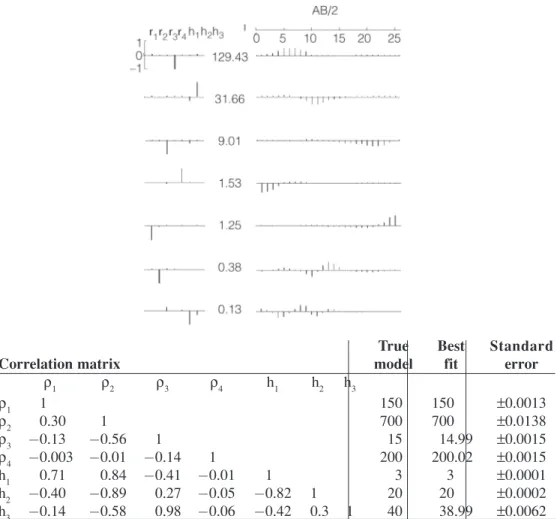
For the second example, we consider four-layer earth model #2: X(150, 700, 15, 200, 3, 20, 40). Figure 4 shows the theoretical data points for this model. The solid curve in Figure 4 is the final fit to the data points, and the final estimated model is close to the original model. Figure 5 illustrates the parameter eigenvectors, eigenvalues, data eigenvectors, parameter correlation coefficients, and model parameter values with estimated standard errors.
In this example, we note five large eigenvalues and two small eigenvalues.
Due to the several high eigenvalues, the inverse interpretation for this model is not very sensitive to noise, but it is very sensitive to model parameter changes. The eigenvectors may
Figure 4 Theoretical data and best fit curve for a four-layer resistivity model #2 with Schlumberger configuration. 103 : : 102 101 100 101 102 103 104 Apparent resistivity, (0hm — m)
Electrode spacing AB/2, (m)
Estimated model ρ= (15, 700, 14.998, 200.023) h : (3, 20, 39, .9969)
Data point Best fit curve
be interpreted as for the three-layer problem. The eigenvectors associated with the small eigenvalues indicate the expected combination of parameters to which the sounding curve is insensitive, and the eigenvectors associated with the large eigenvalues indicate the combinations of parameters to which the problem is highly sensitive. For example, the eigenvector of λ6= 0.38 indicates that if the ρ2value increases while h2decreases, or vice versa, there will be almost no effect on the sounding curve.
B. FIELD EXAMPLE
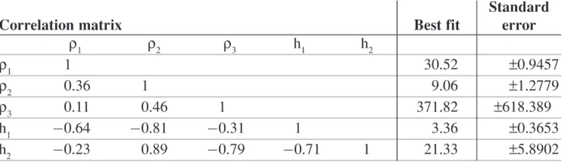
The field data were taken from the Bryson site by Hydro-Québec. Consider the interpretation of the three-layer earth model #3. Figure 6 contains the data for the Schlumberger sounding and its computed sounding curve. The curve fits the data quite well, and the estimated noise level based on this fit is approximately 4 percent of the value at several data points. Since this is considered the approximate accuracy of the data, a closer fit is not justified.
Table 1 illustrates the parameter correlation coefficients, and the model parameter value with estimated standard errors. All calculated parameters may be interpreted as for the three-layer
Figure 5 Parameters and data eigenvectors with associated eigenvalues,
parameter correlations, and best fit model parameters for minimization with standard error weighted data.
True Best Standard
Correlation matrix model fit error
ρ1 ρ2 ρ3 ρ4 h1 h2 h3 ρ1 1 150 150 ±0.0013 ρ2 0.30 1 700 700 ±0.0138 ρ3 −0.13 −0.56 1 15 14.99 ±0.0015 ρ4 −0.003 −0.01 −0.14 1 200 200.02 ±0.0015 h1 0.71 0.84 −0.41 −0.01 1 3 3 ±0.0001 h2 −0.40 −0.89 0.27 −0.05 −0.82 1 20 20 ±0.0002 h3 −0.14 −0.58 0.98 −0.06 −0.42 0.3 1 40 38.99 ±0.0062
problem in model #1. The data do not appear to provide much information about the third layer: we expected a much higher standard deviation for resistivity ρ3. Another interesting observation is the strong correlation between parameter ρ3and the thickness of the second layer.
Figure 6 Field data from the Bryson site (Hydro-Québec) and interpreted best fit curve for three-layer resistivity model #3.
102 101 101 100˚˚˚ 102 model estimated ρ : (30.5, 9.06, 371.82) h: (3.36, 21.33) x : Apparent resistivity measured 0 : Apparent resistivity calculated -- : Best fit curve
Apparent resistivity, (Ohm — m)
Standard
Correlation matrix Best fit error
ρ1 ρ2 ρ3 h1 h2 ρ1 1 30.52 ±0.9457 ρ2 0.36 1 9.06 ±1.2779 ρ3 0.11 0.46 1 371.82 ±618.389 h1 −0.64 −0.81 −0.31 1 3.36 ±0.3653 h2 −0.23 0.89 −0.79 −0.71 1 21.33 ±5.8902
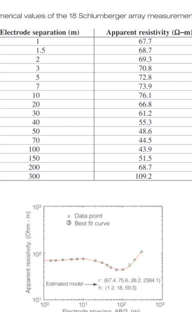
The final example, an interpretation of resistivity sounding measurements, was analyzed for a four-layer case using the Schlumberger configuration in Table 2.
Figure 7 illustrates the measured and calculated apparent resistivities, showing better correlation.
Table 3 illustrates the parameter eigenvectors, eigenvalues, and data eigenvectors. Table 4 illustrates the parameter correlation coefficients and the model parameter value with estimated standard errors.
All calculated parameters may be interpreted as for the four-layer problem in model #2. The data do not appear to provide much information about the fourth layer: we expected a higher standard deviation for the resistivity ρ4. Another interesting observation is the strong correlation between parameter ρ3and the thickness of the second and third layers.
Table 1 Parameter correlations and best fit model parameters for minimization with standard error weighted data
Table 2 Numerical values of the 18 Schlumberger array measurements Electrode separation (m) Apparent resistivity (W--m)
1 67.7 1.5 68.7 2 69.3 3 70.8 5 72.8 7 73.9 10 76.1 20 66.8 30 61.2 40 55.3 50 48.6 70 44.5 100 43.9 150 51.5 200 68.7 300 109.2
Figure 7 Field data and interpreted best fit curve for four-layer resistivity model #4.
Eigenvalues Parameter eigenvectors
r r1 rr2 rr3 rr4 h1 h2 h3 7.243 −0.153 0.038 −0.191 0.736 −0.628 0.015 −0.000 5.452 −0.075 −0.022 −0.474 −0.644 −0.592 −0.592 −0.000 3.280 −0.111 −0.941 −0.069 0.058 0.067 0.297 −0.0007 1.247 −0.000 −0.000 0.0001 −0.0001 −0.0002 −0.003 −1.0000 0.770 0.952 −0.134 0.121 0.028 −0.244 0.0111 −0.000 0.088 0.219 0.039 −0.845 0.192 0.428 −0.125 0.0002 0.0004 0.059 0.304 -0.064 0.027 0.079 0.944 −0.0034
VII. ELECTRODE RESISTANCE EXPRESSIONS
Using an N-layer earth model, as shown in Figure 8, the electrode resistance can be approximated using Wenner’s arrangement.
The general recurrence expression for Wenner apparent resistivity is (j = n − 1, n − 2, ..., 2, 1), (22) (23) ρnaW = ρn (24) (25) where
ρjis the resistivity of the jth layer,
hj is the thickness of the jth layer,
ρjaWis the Wenner apparent resistivity at jth layer,
n is the number of layers in the soil model, and C is the distance between any two electrodes.
The apparent resistivity ρawof the N-layer model is obtained at j = 1:
(26)
where
Reis the ground electrode resistance Ω, and r is the electrode radius m.
The height of the top layer (i.e., h1) varies.
When h1increases, the approximation of the electrode resistance becomes more accurate. When h1approaches infinity (homogeneous soil), the expression reduces to
ρ1aW( )r ≈ρ1 R r r e= ρ1aW( ) 2π H c h i c h i h i ( , , ) ( ) ( ) ( ) j j j = + − + 4 2 2 1 2 1 2 2 2 2 c c kj (j 1)aW j (j 1)aW j = − + + + ρ ρ ρ ρ ρjaW( )c=ρ + ∑k H c h i( , j, ) = ∞ j j i i 1 1 Best Standard
Correlation matrix fit error
ρ1 ρ2 ρ3 ρ4 h1 h2 h3 ρ1 1 67.4 ±0.0029 ρ2 0.3852 1 75.6 ±0.0031 ρ3 0.1525 0.460 1 28.2 ±0.0107 ρ4 0.0218 0.075 0.460 1 2384.1 ±6.7673 h1 0.7656 0.735 0.306 0.045 1 1.2 ±0.0010 h2 −0.3647 −0.7253 −0.902 −0.305 −0.606 1 18 ±0.0046 h3 0.1462 0.4414 0.9846 0.6028 0.2938−0.875 1 59.3 ±0.0378
Table 4 Parameter correlations and best fit model parameters for minimization
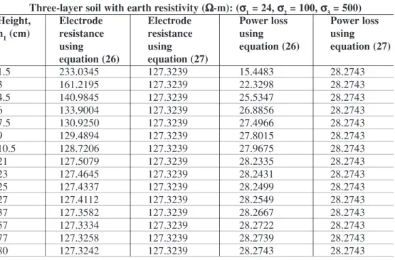
(27) This is the expression for the resistance of hemisphere buried in a homogeneous soil. The computed ground electrode resistance and power loss are tabulated in Table 5 for varying values of h1. R r e= ρ1 2π
Figure 8 Hemisphere buried in N- Layer soil. surface ρ1 ρ2 ρn — 1 hn — 1 h2 h1 ρn V = 60.0 volts r = 0.03 m I r
Table 5 Electrode resistance and power loss vs. height
Three-layer soil with earth resistivity (WW-m): (rr1= 24, rr2= 100, rr3= 500)
Height, Electrode Electrode Power loss Power loss
h1(cm) resistance resistance using using
using using equation (26) equation (27)
equation (26) equation (27) 1.5 233.0345 127.3239 15.4483 28.2743 3 161.2195 127.3239 22.3298 28.2743 4.5 140.9845 127.3239 25.5347 28.2743 6 133.9004 127.3239 26.8856 28.2743 7.5 130.9250 127.3239 27.4966 28.2743 9 129.4894 127.3239 27.8015 28.2743 10.5 128.7206 127.3239 27.9675 28.2743 21 127.5079 127.3239 28.2335 28.2743 23 127.4645 127.3239 28.2431 28.2743 25 127.4337 127.3239 28.2499 28.2743 27 127.4112 127.3239 28.2549 28.2743 37 127.3582 127.3239 28.2667 28.2743 57 127.3334 127.3239 28.2722 28.2743 77 127.3258 127.3239 28.2739 28.2743 80 127.3242 127.3239 28.2743 28.2743
VIII. CONCLUSION
The ridge regression estimator is a powerful method for interpreting resistivity soundings over plane-layered earth structures. Accordingly, it is possible to find a model that fits the data, to indicate the accuracy of the fit relative to the noise level in the data, and to predict the accuracy with which each parameter is estimated.
The inversion method is based on a statistical estimation of the parameters of an N-layer soil model from Schlumberger measurements. This method provides the best estimate of soil parameters.
Finally, computation of the ground electrode resistance of hemisphere buried in N-layer soil is easier and faster using this method.
IX. APPENDIX
In order to obtain a recursive relationship for the partial derivatives, we differentiate Eq. (1):
Using these expressions for j = 2, 3, ..., n, recursive application gives the partial derivatives of raS= rnaS
Introducing Gi(a, b, dj, i) = Gi, we have:
For k = 1, 2, ..., j − 1, we have: W=
k
a b d i = +∞∑
j – 1 i i 1 i j G ( , , , ) ∂ ∂ = − ∂ ∂ + − − − kj 1 ρ ρ ρρ ρ ρ k j (j 1)aS k j (j 1)aS 2 2 ( ) ∂ ∂ = ∑ ∂ ∂ − − − +∞ − ρ ρ jaS j 1 h K G h j aS j i i=1 i j 1 ( 1) 1 B= (2d ij )2+ +(a b)2 A= (2d ij)2+ −(a b)2 ∂ ∂ = − − G hj i B A i U 1 2 3 3 4 dj 1 1 ∂ ∂ = ∑ ∂ ∂ − +∞ − − − ρ ρ ρ jaS j ( 1) =1 1 1 1 j aS i j i i j j iK G K ρρ ∂ ∂ = − + − − − k j aS j j j aS j 1 ρ ρ ρ ρ ( 1) ( 1) 2 2 ( ) ∂ ∂ = + − − − kj j ( 1) ( 1) 1 ρ ρ ρ ρ 2 2 j aS j j ( aS) ∂ ∂ = ∂ ∂ = − + ρ ρ ρ ρ ρ ρ 1aS 1 1 1 1 2 2 1 2 2 and k ( )X. REFERENCES
[1] A. P. Meliopoulos and A. D. Papalexopoulos, Interpretation of soil resistivity measurements: Experience with the Model SOIMP, IEEE Transactions on Power Delivery, Vol. PWRD-1, No. 4, October 1986, pp. 142-151.
[2] F. Dawalibi and N. Barbeito, Measurements and Computations of the performance of Grounding Systems Buried in Multilayer Soils, IEEE Trans. Power Delivery, Vol. 6, No. 4, October 1991, pp 1483-1490.
[3] Takahashi T., Kawase T., Analysis of Apparent resistivity in a Multi-Layer Earth Structure. IEEE Trans. Power Delivery, Vol. 5, No. 2, April 1991, pp 604-610.
[4] Del Alamo J.L., A Comparison among eight different techniques to achieve an optimum estimation of electrical grounding parameters in two-layered earth, IEEE Trans. Power Delivery, Vol. 8, No. 4, October 1993, pp 1890-1899.
[5] P. J Lagacé, J. Fortin, E.D. Crainic, Interpretation of Resistivity Sounding Measurements in N-Layer Soil using Electrostatic Images, IEEE Trans. Power Delivery, Vol. 11, No. 3, July 1996, pp 1349-1170.
[6] F. H. Slaoui, S. Georges, P. J. Lagacé, X. D. Do, “The Inverse Problem of Schlumberger Resistivity Sounding Measurements by Ridge Regression”, Electric Power System Research Journal, Elsevier April 2003.
[7] F. Slaoui, S. Georges, P.J. Lagacé et X.D. Do. (2001). “Fast Processing of Resistivity Sounding Measurements in N-Layer Soil”, The Proceedings of the IEEE Power Engineering Society 2001 Summer Meeting Vancouver, Canada.
[8] P. J. Lagace and M. N. Vuong, “Graphical user interface for interpreting and validating soil resistivity measurements”, the Proceeding of the IEEE, ISIE 2006, Montreal Canada, pp 1841-1845.
[9] D.W. Marquardt, An Algorithm for Least Squares Estimation of Non-Linear Parameters, Journal of the society of Industrial and Applied Mathematics, No.11, 1963, pp. 431-441.
[10] E. D. Sunde, Earth Conduction Effects in Transmission Systems, Dover Publications, New York, 1968.
[11] G. A. F. Seber, C. J. Wild, Nonlinear Regression, New York: Wiley, 1989.
∂ ∂ = ∂ ∂ + − − ρ ρ ρ jaS k h h W Q (j 1)aS k (j 1)aS . . Q ik k h k i = ∂ ∂ + − − = +∞ −