Uncertainties in atomic data and propagation of uncertainties through spectral models

M.A. Bautista1 _{et al.}

Received ; accepted

1_{Department of Physics, Western Michigan University, Kalamazoo, MI 49008, USA} [email protected]

ABSTRACT

We present a method to compute unceratinties in spectral models, i.e. levels populations, line emissivities, and emission line ratios, from propagation of un-certainties in atomic data.. This results from analytic expressions, in the form or linear sets of algebraic equations, for the coupled uncertainties among all levels. These equations efficiently for any set of physical conditions and uncertainties in the atomic data. We illustrate our method in the case of spectral models of O III and Fe II and discuss the general behaviour of the uncertainties under different physical conditions. As to the intrinsic uncertainties in theoretical atomic data, we propose that these uncertainties can be estimated from the dispersion in the results from various independent calculations. This technique is shown to give excellent results for the uncertainties in A-values for forbidden transitions in [Fe II].

1. Introduction

Analysis of observed spectra provides essential information about the behavior and evolution of astronomical sources. By interpreting the spectra one learns about the density and temperature conditions, the chemical composition, the dynamics, and the sources of energy that power the emitting object. For such an interpretation ne needs to to model the excitation and ionization balance of plasmas, out of local thermodynamic equilibrium (LTE), with sufficiently high accuracy. And the accuracy ultimately depends on the quality of the atomic data/molecular employed.

At present, atomic data, of varying accuracy, exists for most processes and spectral lines observed in spectra from the infrared to the X-rays. These data accounts for tens

of thousands of transitions from all ionic stages of most elements of the first five rows of the periodic table. This large amount of data can only be obtained through theoretical calculations, with only a few sparece checks against experimental determinations.

At present, there is no general quantitative approach to estimate uncertainties in theoretical spectral models from uncertainties in atomic data. In recent years, a few authors have presented methods based on the Monte Carlo numerical technique for propagating uncertainties through spectral models, e.g. Wesson, Stock, and Scicluna (2012). Though, these techniques have the disadvantage of being very inefficient, thus their general applicability in highly envolved spectral modeling is limited. Finding a general and efficient method for estimating uncertainties in spectral models is important for two reasons. First, one needs to be able to perform physically realistic comparisons between theoretical and observed spectra, such that reliable conclusions within what the accuracy of atomic/molecular data can be drawn. At present this is not possible, and researchers are restricted to find best fits to observed spectra, without much understanding of the uncertainties in the results. The second reason for uncertainty propagations analysis is that, when dealing with complex and/or very large atomic systems, like ions with multiple metastable levels (e.g. Fe II) and models for UV and X-ray spectra that account for hundreds of highly excited levels, atomic data homogeneously accurate for all transitions can not be obtained. In these cases, error propagation analysis of the spectra could discriminate between critically important atomic rates and very large numbers of inconsequential transitions. Thus, theoretical or i experimental efforts in improving atomic data could target specific rates of significant impact on spectral models, rather than trying to determine all possible rates a once.

The rest of the paper is organized as follows. In Section 2 presents the analytical solution to the uncertainties in level populations of a non-LTE spectral model for assumed

uncertainties in atomic parameters. iIn Section 3 we propose a mechanism to estimate the uncertainties in atomic/molecular data and we test this in the case of Fe II through extensive with observed spectra. In Section 4 we discusse the uncertainties in line emissivities and emission line ratio diagnostics. Section 5 prsents our conclusions. For the sake of simplicity, rest of the paper deals explicitly with the case population balance by electron impact excitation followed by spontaneous radiative decay. It is also assumed that the plasma is optically thin. However, it is noted that our methods can be easily extended to ionization balance computations, additional excitation mechanisms such as continuum and Bowen fluorescence, and optically thick transitions.

2. Uncertainties in Level Populations and Column Densities

Under steady-state, population balance conditions the population, Ni, of a level i is Ni =

!

k!=iNk(neqk,i+ Ak.i)

ne!_j!=iqi,j+!_j<iAi,j, (1)

where ne is the electron density, Ak,i is the Einstein spontaneous radiative rate from level k to level i and qk,i is the electron impact transition rate coefficient for transitions from level k to level i. Here, we assume that the electron velocity distribution follows the Maxwell-Boltzmann function, thus qk,i and qi,k are both proportional to a symmetrical effective collision strength, Υk,i = Υi,k, which is the source of uncertainty in the collisional transition rates. Assuming that the spectral model is arranged in increasing level energy order Ak,i = 0 whenever k < i. We note the that the second term in the denominator of the above equation is the inverse of the lifetime of level i, i.e., τi = (!j < iAi,j)−1_{. This} is important because lifetimes are generally dominated by a few strong transitions, which are much more accurately determined than the weak transitions. Thus, τi carries smaller

uncertainties than individual A-values. Then, equation (1) can be written as Ni =

!

k!=iNk(neqk,i+ Ak.i) neτi!_j!=iqi,j+ 1 τi =

!

k!=iNk(neqk,i+ Ak.i) ne/nc

i + 1

τi, (2)

where nc

i is the so-called critical density of level i and is defined as nci= (τi!j!=iqi,j)−1. The uncertainty in the population of level i, δNi, can be computed as

(δNi)2 =" k!=i #$ ∂Ni ∂Υk,i %2 (δΥk,i)2+ $ ∂Ni ∂Ak,i %2 (δAk,i)2 & +" j!=i $ ∂Ni ∂Ai,j %2 (δAi,j)2+" k!=i $ ∂Ni ∂Nk %2 (δNk)2. (3)

The first three term on the right hand side of this equation represent direct propagation of uncertainties from atomic rates from or to level i. The last term in the equation correlates the uncertainty in level i with the uncertainties in the level populations of all other levels that contribute to it . Then,

$ δNi Ni %2 −" k!=i N_k2(neqk,i+ Ak,i) 2 κ2 $ δNk Nk %2 = 1 κ2 # n2_e" k!=i (Nkqk,i− Niqi,k)2 $ δΥk,i Υk,i %2 +" k>i (NkAk,i)2 $ δAk,i Ak,i %2 + $ N2 i τ2 %2$ δτi τi %2& (4)

where κi =!_k!=iNk(neqk,i+ Ak,i).

This linear set of equations yields the uncertainties to the populations of all levels. Before proceeding to solve these equations it is worth pointing three important properties: (1) uncertainties are obtained relative to the computed level populations regardless of the normalization adopted for these. This is important because while some spectral models compute population relative to the ground level other models solve for normalized populations such that !Nk is either 1 or the total ionic abundance. Though, the equation above is generally applicable regardless of the normalization adopted. (2) In the high density limit, ne → ∞, the right hand side of the equation goes to zero, thus the population

uncertainties naturally go to zero as the populations approach the Maxwell-Boltzmann values (LTE conditions). (3) By having an analytical expression for the propagation of uncertainties one can do a detailed analysis of the spectral model to identify the key pieces of atomic data that determine the quality of the model por any plasma conditions. (4) The set of linear equations for the uncertainties needs to be solved only once for any set pf conditions and it is of the same size as that for the level populations. This is unlike Monte Carlo approches that require solving population ballance equations hundreds of times, which makes real-time computation of uncertanties impractical.

The set of equations above can be readily solved by writing them as

B ¯x = ¯b, (5)

where xi = (δNi/Ni)2, and the matrix and vector elements of B and ¯b are given by the equation 2.

Figure 1 show the populations and population uncertainties for the first four excited levels of O III as a function of the electron density at a temperature of 104 _{K. For} this computation we have assumed 5% uncertainties in the lifetimes, 10% uncertainties in individual A-values, and 20% uncertainties in the effective collision strengths. The levels considered here are 2p2 3_P0,1,2, 1_{D2, and} 1_{S0. It is seen that levels 2 through 5} have maximum uncertainties, ∼20%, in the low density limit where the populations are determined by collisional excitations from the ground level. As the electron density increases thermalization of levels with similar energies and radiative cascades start becoming more important, which diminishes the contribution of uncertainties in collision strengths and ehances the importance of uncertainties in A-values. For high densities all population uncertainties naturally go to zero as the populations approach the Boltzmann limit. Another thing to notice is that, the population uncertainties exhibit multiple contributions and peaks as the metastable levels 3_P

these propagate through higher levels.

Figure 2 show the populations, relative to the ground level, and population uncertainties for the first eight excited levels of Fe II as a function of the i electron density at a temperature of 104 _{K. For these calculation we use atomic data as in Bautista and Pradhan (1998)} we assume uncertainties of 5% in the lifetimes, 10% in individual A-values, and 20% in the effective collision strengths. The levels considered here are 3d6_4s 5_{D9/2,7/2,5/2,3/2 and} 3d7 4_{F9/2,7/2,5/2,3/2. An interesting characteristic of the Fe II system is that the 3d}7 4_F9/2 excited level is more populated, at least according to the atomic data adopted here, than the ground level at densities around 104 _cm−3_{, typical of H II regions. Moreover, under} these conditions only ∼20% of the total Fe II abundance is in the ground level. This means that unlike lighter species, where excitation is dominated by the ground level or the ground multiplet, in Fe II all metastable levels are highly coupled and uncertainties in atomic data are expected to propagate in a highly non-linear fashion.

In Figure 3 we present the population errors for the lowest 52 levels of Fe II at Te = 104 _{K and ne = 10}4 _cm−3_{. These are all even parity metastable levels, except for the} ground level. The figure shows the total estimated uncertainties together with the direct contributions from uncertainties in the collision strengths and A-values (first and second terms on the right hand side of equation 2) and the contribution from level uncertainty coupling. It is observed that the collision strengths are the dominant source of uncertainty for all levels except level 6 (a 4_{F9/2). For this level the uncertainty is dominated by the} A-values and uncertainty couplings with levels of its own multiplet and levels of the ground multiplet. This is important because we find that the a 4_F

9/2 level makes the largest contribution to the uncertainties in 36 of the lowest 52 levels of Fe II. Unfortunately, the atomic data for the 4_{F9/2 level are among the most uncertain parameters of the whole Fe II} system, as we discuss the next section.

2 4 6 8 0 0.2 0.4 0.6 0.8 1 i=2 3 4 5 2 4 6 8 0 0.05 0.1 0.15 0.2 i=2 3 4 5

Fig. 1.— Level populations relative to their Boltzmann limits (upper panel) and relative level population uncertainties (lower panel) for the 2p2 3_{P1 (i = 2),}3_{P2 (i = 3),}1_{D2i (i = 4),} and 1_{S0 (i = 5) excited levels of O III.}

0 0.2 0.4 0.6 0.8 2 3 4 5 2 4 6 8 0 0.05 0.1 0.15 0.2 2 3 4 5 0 0.5 1 1.5 6 7 8 9 2 4 6 8 0 0.05 0.1 0.15 0.2 6 7 8 9

Fig. 2.— Level populations relative to the ground level (upper panel) and relative level population uncertainties (lower panel) for the 3d6_4s6_{D7/2 (i = 2),} 6_{D5/2 (i = 3),} 6_D3/2i (i = 4), 6_D

1/2 (i = 5), 3d7 4F9/2 (i = 6), 3d7 4F7/2 (i = 7), 3d7 4F5/2 (i = 8), and 3d7 4F3/2 (i = 9).

Fig. 3.— Estimated level population uncertainties for the lowest 52 levels of Fe II at Te = 104 K and ne = 104 _{(black line). Here we assume uncertainties for lifetimes, A-values, and} collisional rates of 5%, 10%, and 20% respectively. The figure also depicts the contributions from uncertainties in collisional rates (blue line), A-values (green line), and coupling of uncertainties among all levels (red line).

3. Estimating true uncertainties in atomic data

In the previous section we adopted general uncertainties for lifetimes, A-values for forbidden transitions, and effective collision strengths of 5%, 10%, and 20%, respectively. In absence of generally accepted procedures to estimate uncertainties in theoretical atomic data, these kind of numbers are often cited in the literature as general guidelines; however, uncertainty estimates on specific rates are rarely provided. In Bautista et al. (2009) we proposed that uncertainties in gf-values could be estimated from the statistical dispersion among the results of multiple calculations with different methods and by different authors. The uncertainties can be refined by comparing with experimental or spectroscopic data whenever available, although these also have significant associated uncertainties. This approach is similar to what has been done for many years by the Atomic Spectroscopy Data Center at the Nation Institute of Standards and Technology (NIST; http://www.nist.gov/pml/data/asd.cfm) in providing a ’critical compilations’ of atomic data.

In estimating uncertainties from the dispersion of multiple results one must keep in mind some caveats: (a) Small scatter among rates is obtained when the computations converge to a certain value, yet there is no guarantee that every converged result from approximate calculations will be correct. (b) Large scatter among different calculations is expected in atomic rates where configuration interaction and level mixing lead to cancelation effects. The magnitude of these effects depedns on the wave-function representation adopted. Thus, some computations maybe a lot more accurate than other for certain transitions, while the scatter among all different computations mayoverestimate the tru uncertainty. However, detailed information about configuration and level mixing for every transition is rarely available in the literature. Nevertheless, in absense of complete information about every transition rate from every calculation, a critically comparison between the results of

different calculations and other sources of data, if available, provides a reasonable estimate of the uncertainty in atomic/molecular rates.

Are the statistical dispersion values realistic uncertainty estimates? To answer this question we look at the intensity ratios between emission lines from the same upper limit as obtained from observed astronomical spectra and theoretical predictions. The advantage of looking at these ratios is that they depend only on the A-values, regardless of the physical conditions of the plasma. Thus, the ratios ought to be the same in any spectra of any source, provided that the spectra have been corrected for extinction. Fe II yields the richest spectrum of all astronomically abundant chemical species. Thus, these are the best lines for the present experiment.

One hundred thirty seven [Fe II] lines are found in the HST/STIS archived spectra of the Weigelt blobs of η Carinae. Six medium dispersion plectra (R=6000 to 10,000) of the blobs were recorded between 1998 and 2004 at various orbital phases of the star’s 5.5-year cycle. Seventy eight [Fe II] lines are also present in the deep echelle spectrum (R=???) of the Herbig-Haro object (HH 202) in the Orion nebula from Mesa-Delgadoet al. (2009). The importance of having multiple spectra from different sources and different instruments can not be overestimated. Multiple measurements of the same line ratio minimize the likelihood of systematic errors due to unidentified blends, contamination from stellar emission, and instrumental effects.

From the observations, there are 107 line ratios reasonably well measured from the spectra. The ratios are defined as

ratio = max(F1, F2)/min(F1, F2), (6)

where F1 and F2 are the measured fluxes of two lines from the same upper level. Here, it is important that the minimum of the two fluxes is put in the denominator for the ratio. Thus, the line ratios are unconstrained and they are all equally weighted when comparing

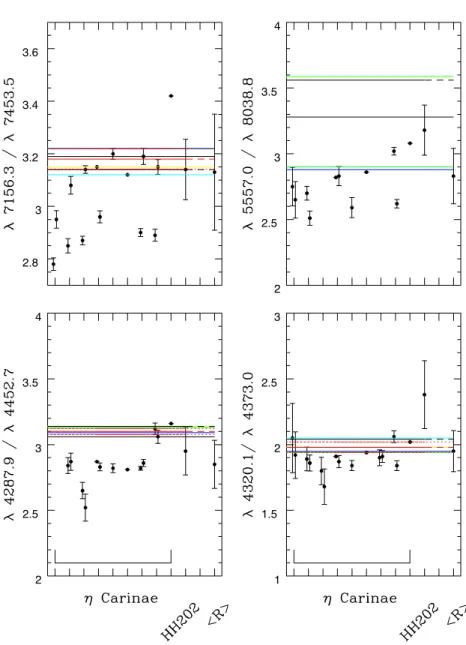
with theoretical expectations. Figure 4 illustrates a few line ratio determinations from several measurements from spectra of η Carinae and HH 202, as well as from various theoretical determinations. In practice, we perform up to four measurements of every observation for different spectral extractions along the CCD, and different assumptions about the continuum and the noise levels. Thus, we see that the scatter between multiple measurements of a given ratio greatly exceed the statistical uncertainties in the line flux integrations. Moreover, the scatter between measured line ratios often exceeds the scatter between theoretical predictions. Full details about the Fe II spectra and measurement procedures will be presented in a forthcoming paper, where we will also present our recommended atomic data for Fe II.

For the present work we consider seven different computations of A-values for Fe II. These are the SUPERSTRUCTURE and relativistic Hartree-Fock (HFR) calculations by Quinet, Le Douneuf, and Zeippen (1996), the recent CIV3 calculation of Deb and Hibbert (2011), and various new HFR and AUTOSTRUCTURE calculations that extend over previous works. Figure 5 presents a sample of theoretically calculated lifetimes and transition yields in Fe II. The yields are defined as yi,j = Ai,j × τi. From the dispersion among various results the average uncertainty in lifetimes for all levels of the 3d7 _and 3d6_{4s configuration is 13%. More importantly, it is found that the the uncertainty in the} critically important a 4_{F9/2 level is∼ 80%, due to of cancelation effects in the configuration} interaction representation of the a 4_F

9/2− a 6D9/2 transition.

We compared the observed lines ratios described above with the predictions from different sets of theoretical A-values. Without uncertainty estimates for the theoretical values, the reduced-χ2 _{values from these comparison range from 2.2 to 3100 for the different} sets of A-values. On other hand, if one adopts average A-values from all calculations and uncertainties from the resultant standard deviations the reduced-χ2 _{is 1.03. This is}

0 0.05 0.1 0.15 3.9 4 4.1 4.2 0.2 0.3 0.4 0.5 0.1 0.12 0.14 0.16 0.18 0.2

Fig. 4.— Emission line ratios from transitions from the same upper level. The first nine points from left to right results from our measured intensities in the HST/STIS spectra of the Weigelt blobs of η Carinae. The tenth point is the measured ratio in the echelon spectrum of HH 202. The last point to the right depicts the average of all measurements and uncertainties given by the standard deviation. The horizontal lines represent the predictions from several different computations of A-values.

indicative of well estimated uncertainties, neither underestimated nor overestimated, and within these uncertainties there is good agreement between theoretical and experimental line ratios. The comparison between observed and theoretical line ratios, including uncertainties, is presented in Figure 6.

Figure 7 shows the estimated lifetime uncertainties for the lowest 52 levels of Fe II. The figure also presents the level population uncertainties that results from the present uncertainties in lifetimes and transitions yields for a plasma with Te= 104 _{K and ne = 10}4 cm−3_{. Here, the adopted uncertainties in the collision strengths are kept at 20% for all} transitions. By far, the most uncertain lifetime is that of the important a 4_{F9/2 level} (i = 6), yet the way that this uncertainty propagates through level populations depends on the density of the plasma. For electron densities much lower than the critical density for the level the uncertainty in the lifetime will reflect directly on the level pollution for that level. This is seen at ne = 104 _cm−3 _{for levels ∼18 and higher However, as the density} increases the uncertainties in the level populations become incresingly dominated the collision strengths. This effect is clearly illustrated in Figure 8.

4. Uncertainties in Emission Line Emissivities and Diagnostic Line Ratios

The line emissivity, in units of photons per second, of a transition i→ f, with i > f, is

ji,f = Ni× Ai,f. (7)

In computing the uncertainty in ji,f one must to account for the fact that Ni and Ai,f are correlated, because the latter appears in the denominator term of Equation (1) that determines Ni. This is important because the most frequently observed lines from any upper level are usually those that dominate the total decay rate for the level, i.e., the

2.8 3 3.2 3.4 3.6 2 2.5 3 3.5 4 2 2.5 3 3.5 4 1 1.5 2 2.5 3

Fig. 5.— Theoretically calculated lifetimes and transition yields in Fe II. The calculations depicted are SST: SUPERSTRUCTURE computation by Quinet, Le Douneuf, and Zeippen (1996); HFR: HFR calculation by Quinet, Le Douneuf, and Zeippen (1996); HFRn: our new HFR calculation; CIV3: results by Deb and Hibbert (2011); ATS21, ATS2, and ATS3: our new AUTOSTRUCTURE calculations that extend over Quinet, Le Douneuf, and Zeippen (1996). The last point to the right of each panel depicts the average value of the various determinations. The uncertainty bars for this point are set by the statistical dispersion between all values.

Fig. 6.— Line ratios between line from the same upper level measured from optical nebular spectra vs. theoretical predictions.

Fig. 7.— The upper panel presents the estimated uncertainties in lifetimes for the lowest 52 levels of Fe II. The lower panel is like Figure 3 but from uncertainties in lifetimes and radiative yields estimated from the dispersion among various calculations.

0 0.2 0.4 0.6 0.8 2 3 4 5 2 4 6 8 0 0.05 0.1 0.15 0.2 2 3 4 5 0 0.5 1 1.5 2 6 7 8 9 2 4 6 8 0 0.2 0.4 0.6 0.8 6 7 8 9

Fig. 8.— Like 2 but from uncertainties in lifetimes and radiative yields estimated from the dispersion among various calculations.

inverse of the level’s lifetime. It is convenient to re-write the above equation as

ji,f = κi Ai,f

ne!_jqi,j+!_jAi,j. (8)

Combining this equation with Equation 2 we find $ δji,f ji,f %2 = $ δNi Ni %2 + $ Ni κiτi %2$ δτi τi %2 + $ 1₋ Ni κiAi,f %2$ δAi,f Ai,f %2 . (9)

This equation can be readily evaluated from the level populations and uncertainties already known. The equation has varios interesting properties: (1) the equation is independent of the physical units used for the emissivities; (2) in the high density limit, as the uncertainty in the level population goes to zero, the uncertainty in the emissivity is the same as in the A-value.

Figure 9 depicts uncertainties in emissivity for a sample of strong IR, near-IR, and optical [Fe II] lines. These are computed at 104 _{K. The uncertainties in the collision} strengths are 20% and the uncertainties in the lifetimes and A-values are those estimated in the previous section. The behavior of these uncertainties for different physical conditions is complex. Let us look, for instance, at the uncertainty of emissivity of the 5.3µm line (a 4_{F9/2− a} 6_{D9/2; 6 → 1) whose behavior is contrary to uncertainty in the pollution of the} a4F

9/2 level (see Figure 8). According to equations 2 and 4, in the low density limit ji,f _→" k Nkneqk,i ' Ai,f ! jAi,j ( . (10)

In the case of the a 4_{F9/2 level the 5.3µm transition dominates the total decay rate of level} and the ratio Ai,f/!_jAi,j is essentially 1. Thus, the uncertainty in the A6,1 rate cancels out at low electron densities and the uncertainty in the emissivity is small despite a large uncertainty in the level population. By contrast, at high densities the population of the level approaches the Boltzmann limit and the uncertainty in the emissivity is solely given by that in A6,1, which is ∼ 80%.

0 0.05 0.1 0.15 (a) 0 0.2 0.4 0.6 0.8 1 (b) 0.18 0.2 0.22 0.24 0.26 (c) 0.1 0.15 0.2 0.25 (d) 0 0.2 0.4 0.6 0.8 (e) 0 0.2 0.4 0.6 0.8 (f) 2 4 6 8 0.1 0.15 0.2 0.25 0.3 (g) 2 4 6 8 0 0.05 0.1 0.15 0.2 0.25 (h)

Fig. 9.— Uncertainties in [Fe II] line emissivities at 104_{vs. n}

e. The transitions shown are: (a) 25.9 µm (a6_D7/2−a6_{D9/2); (b) 5.33 µu (a}4_F9/2−a6_{D9/2); (c) 1.256 µm (a}4_D7/2−a6_D9/2); (d) 8616.8 ˚A(a4_P5/2−a4_{F9/2); (e) 7155.2 ˚A(a}2_G9/2−a4_{F9/2); (f) 5527.4 ˚A(a}2_D5/2−a4_F7/2); (g) 4889.7 ˚A(b 4_P

A line emission ratio between two lines is given by R = ji,f jg,h = $ Ni Ng % $ Ai,f Ag,h % $ ∆Ei,f ∆Eg,h % , (11)

where ∆Ei,f is the energy difference between levels i and f and we have use emissivties in units of energy per second. In computing the uncertainty in this line ratio one must account for the fact that the emissivieties are correlated. Moreover, a general expresion for the uncertainty must account for cases where i = g, in which case the uncertainty in the ratio would depend only on the A-values. The uncertainty is the ratio is given by

$ δR R % = ) 1− R $ ∂jg,h ∂ji,f %*2$ δji,f ji,f %2 + ) 1− R $ ∂ji,f ∂jg,h %*2$ δjg,h jg,h %2 , (12) where ∂ ∂ji,f = 1 Ai,f ∂ ∂Ni + 1 Ni ∂ ∂Ai,f. Thus, $ δR R % = ) 1− R $ Ag,h∆Eg,h Ai,f∆Ei,f ∂Ng ∂Ni + Ag,h∆g,h ∆Ei,fNi ∂Ng ∂Ai,f %*2$ δji,f ji,f %2 + ) 1− R $ Ai,f∆Ei,f Ag,h∆Eg,h ∂Ni ∂Ng + Ai,f∆i,f ∆Eg,hNg ∂Ni ∂Ag,h %*2$ δjg,h jg,h %2 . (13)

From Equation 2 we find (∂Ni/∂Ag,h) = NiNg/κi for h = i, =−Ni2/κi for g = i, and = 0 otherwise.

In the general case of a ratio involving several lines in the numerator and/or denominator, i.e., R = ! {i,f}ji,f ! {g,h}jg,h , (14) the uncertainty is $ δR R %2 =" {i,f} '!

{i,f}!(∂j{i,f}!/∂j_{i,f})

! {i,f}j{i,f} − ! {g,h}(∂j{g,h}/∂j{i,f}) ! {g,h}j{g,h} (2 δj_{i,f}2 " {g,h} '! {g,h}!(∂j{i,f}!/∂j_{g,h}) ! {g,h}j{g,h} − ! {g,h}!(∂j{g,h}!/∂j_{g,h}) ! {g,h}j{g,h} (2 δj_{g,h}2 (15)

0 0.5 1 1.5 2 2.5 2 4 6 8 0.2 0.4 0.6 0.8 0 1 2 3 2 4 6 8 10 0.24 0.26 0.28 0.3 0.32 0 0.2 0.4 0.6 0.8 1 2 4 6 8 10 0.2 0.4 0.6 0.8 1

Fig. 10.— [Fe II] emissivity line ratios (upper panel) and uncertainties (lower panel) at 104 K vs. electron density.

Figure 10 shows a sample of line ratios between IR and optical lines and their uncertainties. The uncertainties exhibit complex behaviour with changes in density and temperatures. In gerenral, line ratios are only useful as diagnostics when the observed ratio lies near the middlerange of the theoretical ratio. Moreover, it is very important to know the uncertainties in the ratios when selecting appropriate diagnostics from a given spectrum.

5. Conclusions

We presented a method to compute uncertainties in spectral models from uncertainties in atomic/molecular data. Our method is very efficient and allows us to compute uncertainties in all level populatoions by solving a sigle algebraic equation. Specifically, we treat the case of non-LTE models where electron impact excitation is balanced by spontaneous radiative decay. However, the method can be extended to ionization balance and additional excitation mechanisms.

Our method is tested in O III and Fe II models, first by assuming coomonly assumen uncertainties and then by adopting uncertainties in lifetims and A-values given by the dispersion between the results of multiple independent computations. Moreover, we show that uncertainties taken this way are in practice very good estimates.

Then we derive analytic expresions for the uncertainties in line emissivities and line ratios. These equations take into account the correlations between level populations and line emissivities. Interestingly, the behaviour of uncertainties in level populations and uncertainties in emissivities for transitions from the same upper levels are often different and even opposite. This is the case, in particular, for lines tha result from transitions that dominate the total dacay rate of the upper levl. Then, the uncertainties in A-values for the

transitions that yield the lines cancel out with the uncertainties in the lfetims of the levels. In terms of emission line ratios, it is also found that knowledge of the uncertainties in the ratios is essential selecting appropriate ratios s density and temperature diagnostics.

At present, we are in the process of estimating uncertainties in atomic data for species of astronomical interest. Our uncertaonty estimates and analysis of the uncertainties in various spectral models, ionic abundance determinations, and dianostic line ratios will be presented in future publicaitons.

We acknowledge financial support from grants from the NASA Astronomy and Physics Research and Analysis Program (award NNX09AB99G).

REFERENCES

Bautista, M. A., Quinet, P., Palmeri, P., Badnell, N. R., Dunn, J., and Arav, N., 2009, A&A, 598, 1527

Bautista, M. A. and Pradhan, A. K., 1998, ApJ, 492, 650 Deb, N. C. and Hibbert, A., 2011, A&A, 536, A74

Mesa-Delgado, A. and Esteban, C. and Garc´ıa-Rojas, J., Luridiana, V. and Bautista, M., Rodr´ıguez, M., L´opez-Mart´ın, L., and Peimbert, M., 2009, MNRAS, 395, 855 Quinet, P. Le Dourneuf, M., and Zeippen, C. J., 1996, A&AS, 120, 361

Wesson, R., Stock, D. J., and Scicluna, P., 2012, MNRAS, 422, 3516