HAL Id: hal-01925325
https://hal.archives-ouvertes.fr/hal-01925325
Submitted on 16 Nov 2018
HAL is a multi-disciplinary open access
archive for the deposit and dissemination of
sci-entific research documents, whether they are
pub-lished or not. The documents may come from
teaching and research institutions in France or
abroad, or from public or private research centers.
L’archive ouverte pluridisciplinaire HAL, est
destinée au dépôt et à la diffusion de documents
scientifiques de niveau recherche, publiés ou non,
émanant des établissements d’enseignement et de
recherche français ou étrangers, des laboratoires
publics ou privés.
A LNS and branch-and-check approach for a VRP with
cross-docking and ressource synchronization
Philippe Grangier, Michel Gendreau, Fabien Lehuédé, Louis-Martin Rousseau
To cite this version:
Philippe Grangier, Michel Gendreau, Fabien Lehuédé, Louis-Martin Rousseau. A LNS and
branch-and-check approach for a VRP with cross-docking and ressource synchronization. INFORMS TSL
Workshop on “E-Commerce and Urban Logistics”, 2018, Hong-Kong, China. �hal-01925325�
A LNS and branch-and-check approach for a VRP with cross-docking and
ressource synchronization
Philippe Grangiera,b,c, Michel Gendreaub, Fabien Lehuédéa,∗, Louis-Martin Rousseaub
aInstitut Mines-Telecom Atlantique, LS2N, UMR CNRS, Nantes, France bCIRRELT, Ecole Polytechnique de Montréal, Montréal, QC, Canada
cJDA, Montréal, QC, Canada
Resource synchronization constraints are a major rising features of many city logistics and transportation problems. Such type of constraints typically arise from limited parking spaces at logistics warehouses or hubs
1. Introduction
In logistics, cross-docking is a distribution strategy in which goods are brought from suppliers to an intermediate transshipment point, the so-called cross-dock, where they may be transferred (without storing) to another vehicle for delivery. Compared to traditional distribution systems, cross-docking can help reducing delivery costs and delivery lead time, that is why it is used by many companies from different sectors: LTL, retail or automotive for example [? ]. In the vehicle routing literature, the associated routing problem is called the Vehicle Routing Problem with Cross-Docking (VRPCD). It is a variant of the Pickup and Delivery Problem with Transfers with one compulsory transfer point: vehicles start by collecting items, then return to the cross-dock where they unload/reload some items and eventually visit delivery locations. A few authors have proposed methods to solve this problem or variants of it, but to our knowledge, in most models there is no limit on the processing capacities of the cross-dock: as soon as a truck arrives, it immediately undergoes consolidation operations. However in practice, this may not be the case because of limited equipment or workforce, and trucks may have to wait before being unloaded. In fact, a wide range of the cross-docking literature is dedicated to the scheduling of operations at the cross-dock taking into account the cross-dock capacity. It has recently been pointed out [? ? ], that there is a need to consider the synchronization of local and network-wide cross-docking operations, in particular to take into account resource capacity at the cross-dock. To that end, in this paper, we introduce a new variant of the VRPCD in which the number of vehicles that can simultaneously be processed at the cross-dock is limited. We call it the Vehicle Routing Problem with Cross-Docking and Resource Constraints (VRPCD-RC). The dock resource constraint, is a
resource synchronization constraint as defined by Drexl [? ] as vehicles compete to access a scarce resource:
the processing capacity of the cross-dock. Very often resource synchronization constraints imply a difficult scheduling problem which is embedded within the vehicle routing problem. VRPCD-RC is no exception and the main contribution of this paper is on the integration of the scheduling problem associated with the dock resource constraints within a recently proposed large neighborhood search based method [? ] for the VRPCD. The remainder of this paper is organized as follows. A literature review is presented in Section 2, while the problem is defined in Section 3. In Section 4, we recall the method of [? ], and Section 5 is devoted to the its adaptation to VRPCD-RC. Eventually, computational results are presented in Section 6.
2. Literature review
In this section we review the literature on two related vehicle routing problems: the vehicle routing problem with cross-docking and vehicle routing problems with resource synchronization.
∗Presentator, corresponding author
Email addresses: philippe.grangier@mines-nantes.fr (Philippe Grangier), michel.gendreau@cirrelt.ca (Michel Gendreau), fabien.lehuede@ls2n.fr (Fabien Lehuédé), louis-martin.rousseau@polymtl.ca (Louis-Martin Rousseau)
2.1. The vehicle routing problem with cross-docking
A lot of cross-docking related problems exist such as: location, assignment of trucks to doors, inner flow optimization or routing. In particular, the vehicle routing problem with cross-docking consists in designing routes to pick up and deliver a set of transportation requests at minimal cost using a single cross-dock. It was introduced by Lee et al. [? ] in a variant which imposes trucks to arrive at the exact same time at the cross-dock. Wen et al. [? ] relaxed this last constraint only imposing precedence constraints based on the consolidation decisions and added time windows. This is the most studied variant, and it is the one we will refer to as the vehicle routing with cross-docking (VRPCD). Several heuristics have been proposed to solve it: based on tabu-search [? ? ? ? ], iterated local search [? ] and large neighborhood search [? ]. Other variants have been studied by Santos et al. [? ? ] which integrate a cost for transferring item at the cross-dock and have no temporal constraints. It was later extended in [? ] with optional cross-dock return. These three articles proposed methods based on branch-and-price. The work of Petersen and Ropke [? ] considers optional cross-dock return and multiple trips per day. They propose a parallel adaptive large neighborhood search to solve large real-life instances with up to 982 requests. In [? ], Nikolopoulou et al. considers optional cross-dock returns when comparing direct shipping versus cross-docking strategy. Dondo and Cerdà [? ] consider a case where the number of doors is fixed and smaller than the number of trucks. In particular each door is modeled individually: a time matrix models the time spent by a truck for moving from an inbound door a to an outbound door b. They solve two randomly generated instances with up to 70 requests with a mathematical model combined with a sweep heuristic. Recently, Maknoon and Laporte [? ] study the extension of the problem to multiple cross-docks, Nikolopoulou et al. study the many-to-many case and Ahmadizar et al. [? ] propose a hybrid genetic algorithm for the multiple cross-dock, multiple suppliers case. From a general perspective, the VRPCD can be viewed as a special case of the pickup and delivery problem with transfers with only one compulsory transfer point [? ]. Guastaroba et al. [? ] released a survey on intermediate facilities in freight transportation. For a general overview of cross-docking and cross-dock related problems we refer the reader to [? ? ? ]
2.2. Resource synchronization
The expression resource synchronization appears in [? ] as a way to model the following constraint: ‘The total consumption of a specified resource by all vehicles must be less than or equal to a specified limit.’
Of course, this resource has to be scarce to be constraining, as vehicles compete to access it. Such resource constraints arise in many different vehicle routing problems usually when a special infrastructure or equipment is required: a docking station or parking space in airport cargo system [? ], a berth in maritime transportation [? ], a forest loader in forestry [? ], a pump in ready mix-concrete delivery [? ], an asphalt paver in public works [? ]. Limited storage [? ] or processing capacities [? ] can also account for resource synchronization constraints. Hempsch and Irnich [? ] also mention a situation where only a fixed number of vehicles (smaller than the total number) can perform long routes.
Many approach have been applied to deal with these resource constraints in vehicle routing problems. In [? ], Ebben et al. sequentially insert requests and check resource constraints in a predefined order. In [? ], El Hachemi et al. use a dedicated constraint programming model, later combined with a greedy scheduling heuristic in [? ], to ensure that resource constraints are satisfied during their entire solving process. In ready-mix concrete routing problems as well as in public works routing problem, orders are larger than truck capacity, as such they have to be split into several delivery operations that should not overlap. Resource synchronization constraints arise at pickup sites or at delivery sites or at both. Asbach et al. [? ], Schmid et al. [? ], Schmid et al. [? ] and Grimault et al. [? ] impose precedence constraints on the sequencing of operations to handle precedence constraints. Gronhaug et al. [? ] rely on a time-discretized formulation in which resource synchronization constraints are easily expressed. Hempsch and Irnich [? ] proposed a generic modeling for inter-routes constraints via the use of Resource Extension Functions (REF). In particular they focused on the use of REF as efficient feasibility tests in local search based algorithms when the solution is represented by a giant tour. From this literature review, it is clear that most of the resource synchronization constraints are in fact complex scheduling problem integrated into a vehicle routing problem. However the precise definition of the scheduling problem depends largely on the vehicle routing problem at stake.
3. The vehicle routing problem with cross-docking: model and resource synchronization con-straint
This section presents the vehicle routing problem with cross-docking, and in particular the cross-dock model, as defined by Wen et al. [? ]. It also introduces the two considered cross-dock resource models .
3.1. The vehicle routing problem with cross-docking
In the VRPCD, we consider a cross-dock c, a set of requests R, and a homogeneous fleet of vehicles V , each of capacity Q and based at o. Each request r ∈ R has to be picked up at its pickup location pr within its pickup time window [epr, lpr], and has to be delivered at its delivery location dr within its delivery time
window [edr, ldr]. In case of early arrival, a vehicle is allowed to wait, but late arrivals are forbidden. We
denote by P the set of pickup locations and by D the set of delivery locations.
Each vehicle starts at o, then goes to several pickup locations, arrives at the cross-dock where it unloads/reloads some requests. A vehicle then visits delivery locations and eventually returns at o. Note that a vehicle has to visit the cross-dock even if it does not unload nor reload any requests there. The sequencing of operations at the cross-dock is described in 3.2. The VRPCD is defined on a directed graph G = (V, A), with G = {o}∪P ∪{c}∪D and A = {(o, p)|p ∈ P } ∪ P × P ∪ {(p, c)|p ∈ P } ∪ D × D ∪ {(d, e)|d, e ∈ D} ∪ {(d, o)|d ∈ D} ∪ {(o, c), (c, o)}. With each arc (i, j) ∈ A is associated a travel time ti,j and a travel cost ci,j.
Solving the VRPCD involves finding |V | routes, and a schedule for each route, such that the capacity and time-related constraints are satisfied, at minimal routing cost. An arc-based mathematical formulation can be found in [? ].
3.2. Precedence constraints at the cross-dock
Following [? ], if a vehicle k has to unload a set of items R−k and reload a set Rk+at the cross-dock, the time spent at the cross-dock can be divided into four periods:
• Preparation for unloading. The duration δu of this period is fixed.
• Unloading of requests. The duration of this period depends on the quantity of items to unload. For vehicle k the duration is (P
i∈R−k qi)/su, where su is the unloading speed in quantity per time unit. All unloaded items become available for reloading at the end of this period.
• Preparation for reloading. The duration δrof this period is fixed.
• Reloading of requests. The duration of this period depends on the quantity of items to reload. For vehicle k the duration is (P
i∈R+kqi)/sr, where sr is the reloading speed in quantity per time unit. All the items for loading must have been unloaded before the beginning of the reloading operation (preemption is not allowed).
Items that are not transferred at the cross-dock remain in the vehicle. Thus, if a vehicle does not unload or reload it need not spend any time at the cross-dock and can leave immediately.
3.3. Resource constraints models at the cross-dock
According to Van Belle et al. [? ], the most common service mode of a cross-dock is called exclusive. In an exclusive mode, a dock door is either exclusively dedicated to unloading (inbound operations) or reloading (outbound operations). Such affectation is a decision taken at a strategical or tactical level which cannot be modified in the VRPCD, which is an operational problem. In practice most cross-docks are I-shaped [? ], with inbound doors on one side and outbound doors on the other. The flow of items is thus uni-directional, which can be easier to manage. This is a common situation but it is not mandatory.
Cross-docks usually have many doors (typically ranging from 40 to 150 according to [? ]). However, as mentioned in [? ] or [? ], processing capacities may actually be lower than the number of doors. This comes from a limited workforce or special equipment to move the items within the cross-dock.
Because of the previous two considerations regarding operations at the cross-dock, we will consider two exclusive cross-dock models that integrate resource constraints:
• a case in which the total number of doors (both inbound and outbound) that can be processed simultaneously is limited to a number S. This is a simple way to model resource constraints due to limited workforce. We refer to this case as shared.
• a case in which the number of inbound doors (resp. outbound doors) that can be processed simultaneously is limited to a number I (resp O). This is a simple way to model a resource constraints due to special equipment. We refer to this case as separated.
Provided that at least two dock doors can be processed simultaneously, the scheduling problems at the cross-dock is NP-Hard as the scheduling problem P 2||Cmax is included in them. In the rest, we will simply use dock to refer to the capacity in the number of docks processed simultaneously.
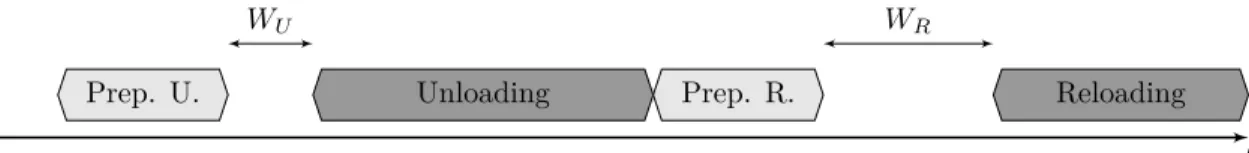
We call the VRPCD with these dock resource constraints, vehicle routing problem with resource constraints (VRPCD-RC). Figure 1 illustrates the sequencing of consolidation operations for a vehicle that unloads and reloads items at the cross-dock in the VRPCD-RC. When the vehicle arrives at the cross-dock, it can immediately be prepared for unloading, but it has to wait before being actually unloaded (WU) because of a lack of available resources (note that such waiting time does not exist in the VRPCD). Once the unloading operation is done, the vehicle can proceed and move to an outbound door. Again preparation operation can be performed immediately, but it may wait before being actually reloaded (WR). This waiting time can have two origins: first, not all items are available when it is ready (such situation can also arise in the VRPCD), second, there maybe a lack of available resources (which cannot occur in the VRPCD).
Prep. U. Unloading Prep. R. Reloading
WU WR
t
Figure 1: Time chart for vehicle unloading and reloading at the cross-dock in the VRPCD-RC
4. Matheuristic of Grangier et al. [? ] for the VRPCD
In a previous paper [? ], we proposed a matheuristic to solve the VRPCD, called LNS+SPM (Large Neighborhood Search + Set Partitioning and Matching). To our knowledge, this method is currently one of the best heuristic for the VRPCD. A sketch of LNS+SPM method is given in Algorithm 1. In details, the main component is LNS(l. 4-15), which is enhanced by the occasional solution of an SPM(l.18 and l.23). When the LNS finds a new solution, the pickup part and delivery part, called legs, of each route are added to a memory component (l. 16), called a pool of legs. The SPM aims to create the best possible solution from the legs in the pool. As shown in [? ], this component significantly improves the quality of the solution compared to LNS alone. Hereafter, we recall the methods that are used in the LNS component and the SPM component.
4.1. Large neighborhood search
Large Neighborhood Search [? ] iteratively destroys (removes several requests from) and repair (reinserts requests into) the current solution using heuristics. In what follows, the destruction and repair methods used in [? ] are summarized.
4.1.1. Destruction operators
When partially destroying a solution, a destruction method M− and a number Φ of requests to remove are selected. Unless stated otherwise, this method is reused until Φ is reached. The transfer removal was introduced for the VRPCD, and the other removal techniques below are inspired by [? ].
Result: The best found solution s?
1 Pool of legs L := ∅
2 Generate an initial solution s 3 s?:= s
4 while stop-criterion not met do 5 s0:= s
6 Destroy quantity: select a number Φ of requests to remove from s0
7 Operator selection: select a destruction operator M− and a repair operator M+
8 Destruction : apply M− to remove Φ requests from s0, and put them in the requests bank of s0 9 Repair: apply M+ to reinsert the requests in the requests bank in s0
10 if acceptance criteria is met then 11 s := s0
12 end
13 if cost of s0 is better than cost of s? then 14 s?:= s0
15 end
16 Add legs of s0 to L
17 if set partitioning and matching condition is met then 18 Perform set partitioning and matching with the legs in L 19 Update s? and s if a new best solution has been found 20 Perform pool management
21 end
22 end
23 Perform set partitioning and matching with the legs in L 24 Update s? if a new best solution has been found
25 return s?
Algorithm 1: LNS+SPM of Grangier et al.
Worst removal:. a request with a high removal gain is removed. The removal gain is defined as the difference
between the cost of the solution with and without the request. Then, the requests are sorted in non increasing order of their removal gains and put in a list N . The request to remove is selected in a randomized fashion as in [? ]: given a parameter p, a random number y between 0 and 1 is drawn. The request in position yp× |N | is then removed.
Historical node-pair removal:. each arc (u, v) ∈ G is associated with the cost of the cheapest solution it
appears in (initially this cost is set to infinity). For each request, the sum of the cost of its associated arcs in the current solution is computed. A randomized selection, similar to worst removal, is performed.
Related removals:. these methods aim to remove related requests. Let the relatedness of requests i and j
be R(i, j). Two distinct relatedness measures are used: distance and time. The distance measure between two requests is the sum of the distance between their pickup points and the distance distance between their delivery points. The time measure is the sum of the absolute difference between their start of service at their pickup points and the absolute gap between their start of service at their delivery point. In both cases a small R(i, j) indicates a high relatedness. A randomized selection, similar to worst removal (albeit with a non decreasing ordering), is performed.
Transfer removal:. for each pair of routes (vi, vj), with vi6= vj the number of requests transferred from vi to
vj is computed. Then a roulette wheel selection is applied on the pairs of routes (the score of a pair being the number of requests transferred), and the requests that are transferred between the routes in the selected pair are removed. If there are less transferred requests than the target number Φ to remove, the rest of the removals is performed with random removal.
4.1.2. Repair operators
In LNS, the unplanned requests are stored in a requests bank. In the following, the operators to reinsert them in a solution are described. Best-insertion, 2-regret, 3-regret and 4-regrets are used as repair methods in LNS+SPM.
Best insertion:. from the requests r in the requests bank, the one with the cheapest insertion cost considering
all possible insertion (with and without transfer) is performed.
Regret Insertion:. for each request r in the requests bank and for each pair of vehicles (pickup vehicle, delivery
vehicle), the cost of cheapest feasible insertion (if any) is computed. Note that the pickup and delivery vehicles may be the same (in the case of insertion without transfer). Then, with these insertion options, the k-regret
value of r is defined as ckr =Pki=1(fi− f1), where f1 is the cost of the cheapest insertion, f2 is the cost of the
second-cheapest insertion and so on, and k is a parameter. The cheapest insertion of the request with the highest regret value is performed.
4.1.3. Feasibility tests and reduction of neighborhood
In [? ], we used an adaptation of forward time slacks [? ] due to Masson et al. [? ] to check time feasibility of insertions in constant time (capacity check in constant time is straightforward). To reduce the runtime, we do not consider all insertions with transfer. For a request r we only consider transfer from the five closest vehicles to its pickup point, to the five closest vehicles from its delivery point. For large scale instances, this halves the runtime.
4.2. Set Partitioning and Matching
Given a set of legs L, set partitioning and matching (SPM) aims to select a subset ˜L of L such that (1)
each request is picked up and delivered by exactly one leg in ˜L and (2) legs in ˜L can be matched to form
routes that respect time constraints. Each leg l ∈ L has an associated routing cost cl, the objective in the SPM is to minimize the sum of the costs of the selected legs. Notice that only non-dominated legs in L have to be considered in the SPM. A pickup (resp. delivery) leg li is said to be dominated by a leg lj iff: li and lj serve the same set of requests, cj< ci and aj ≤ ai (resp. bj ≥ bi) where a represents the arrival time at the cross-dock and b represents the departure time from the cross-dock.
The SPM is solved using a technique called branch-and-check, presented in Section 4.2.1. Its subproblem is a dedicated matching and scheduling subproblem, detailed in Section 4.2.2. The SPM is solved every thousand iterations with a time limit of ninety seconds. If the SPM is solved to optimality within the time limit, the legs in memory are kept, otherwise the pool is cleared.
4.2.1. Branch-and-check
We present branch-and-check [? ] using the following optimization problem:
M 1 : min c|x (1)
Ax ≤ b (2)
H(x, y) (3)
x ∈ {0, 1}n (4)
y ∈ Rm (5)
Assume that H(x, y) represents a set of constraints that have a limited impact on the LP relaxation and/or are difficult to efficiently model in a MIP, but that can be handled relatively easily by a CP solver. (1), (2) and (4) form a relaxation (M2) of (M1) that can be solved using branch-and-bound. The general principle of branch-and-check is the following. To solve (M1), a branch-and-bound is carried on (M2). Whenever an integral solution of (M2) is found, a CP solver is called to check constraints (3). If they are satisfied, the best solution found so far for (M1) is updated accordingly. Otherwise, this solution is rejected. In both cases the branch and bound process continues.
4.2.2. Application of branch-and-check to the VRPCD
For the SPM in the VRPCD, a classical set partitioning problem (SPP) is used as relaxation. For each request r ∈ R and each leg l ∈ L, let λr,lbe a binary constant that indicates whether this request is served by this leg, and for each leg, let xl be a boolean variable that indicate whether this leg is selected. The SPP on legs is then : minX l∈L clxl (6) X l∈Lp λr,lxl= 1 ∀r ∈ R (7) X l∈Ld λr,lxl= 1 ∀r ∈ R (8) xl∈ {0, 1} ∀l ∈ L (9)
The objective (6) is to minimize the cost of the selected legs while constraints (7) (resp. (8)) ensure that each pickup point (resp. delivery point) is covered by exactly one leg.
A solution to the SPP on legs, which involves a set of pickup legs denoted ˜Lp and a set of delivery legs denoted ˜Ld, is a solution to the VRPCD iff there exists a matching of pickup legs and delivery legs to form routes that respects time constraints. For each pickup leg l ∈ ˜Lp, let Tl be the set of delivery legs that deliver at least one request picked up by l. If a pickup leg l and a delivery leg l0 are matched together to create a route, there are an associated unloading task o−ll0, with a set of requests R−ll0 being unloaded, and a reloading
task o+ll0, with a set of requests R
+
ll0 being reloaded. These tasks have to be performed iff l and l0 are in the
same route.
The matching and scheduling problem is modeled as a constraint satisfaction problem, represented using notation from OPL (Optimization Programming Language [? ]). In particular the model is based on the notion of interval variables and uses alternative constraints. As used here (from [? ]):
‘An interval variable represents an interval of time during which a task happen, and whose position in time is an unknown of the scheduling problem. An interval is characterized by a start value, an end value and a size. (...) An interval variable can be optional, that is, one can decide not to consider [it] in the solution schedule.’
In this model, we model alternative activities [? ] by using alternative constraints (from [? ]):
‘An alternative constraint between an interval variable a and a set of interval variables b1, . . . , bn models an exclusive alternative between b1, . . . , bn. If interval a is present, then exactly one of intervals b1, . . . , bn is present and a starts and ends together with this specific interval. Interval a is absent if and only if all intervals in b1, . . . , bn are absent.’
The matching and scheduling problem is then:
Alternative(tl, {o−ll0; ∀l0∈ ˜Ld}) ∀l ∈ ˜Lp (10) Alternative(tl0, {o+ ll0; ∀l ∈ ˜Lp}) ∀l0 ∈ ˜Ld (11) o−ll0.IsOptional ← T rue ∀l ∈ ˜Lp, ∀l0 ∈ ˜Ld (12) o+ll0.IsOptional ← T rue ∀l ∈ ˜Lp, ∀l0 ∈ ˜Ld (13) o−ll0.IsP resent ⇐⇒ o + ll0.IsP resent ∀l ∈ ˜Lp, ∀l0 ∈ ˜Ld (14) tl0.Start ≥ tl.End ∀l ∈ ˜Lp, l0∈ Tl (15) o+ll0.Start ≥ o−ll0.End + δr ∀l ∈ ˜Lp, ∀l0∈ ˜Lds.t. R+ll0 6= ∅ (16) o+ll0.Start ≥ o − ll0.End ∀l ∈ ˜Lp, ∀l0∈ ˜Lds.t. R+ll0 = ∅ (17) o−ll0.Start ≥ al+ δu ∀l ∈ ˜Lp, ∀l0∈ ˜Lds.t. R−ll0 6= ∅ (18) o−ll0.Start ≥ al ∀l ∈ ˜Lp, ∀l0∈ ˜Lds.t. R−ll0 = ∅ (19) o+ll0.End ≤ b0l ∀l ∈ ˜Lp, ∀l0 ∈ ˜Ld (20)
For each pickup leg l, tl is an interval variable that represents the associated unloading task that takes place at the cross dock. Alternative constraints (10) and (12) ensure that for each pickup leg l exactly one unloading task oll0 is scheduled and that it is equal to tl. The same holds for delivery legs and reloading
operations through variables tl0 and constraints (11) and (13). Constraints (14) ensure that the unloading
operation associated with the matching of pickup leg l and the delivery leg l0 in the same vehicle is present iff the corresponding reloading operation is present as well. Constraints (15) ensure that all the reloading operations that depend on a pickup leg l start no earlier than the end of the unloading task associated with l. Constraints (16) and (17) ensure that when two legs are packed together, the delay between the two tasks respects the model presented in Section 3.2. Constraints (18) and (19) ensure that for each pickup leg, its corresponding unloading operation cannot start before the earliest feasible arrival time at the cross-dock. Constraints (20) ensure that for each delivery leg, its corresponding reloading operation is done by its latest feasible departure time.
5. Proposed matheuristic for the VRPCD-RC
In this section, we present the matheuristic that has been derived from [? ] for the VRPCD-RC: Large Neighborhood Search+Set Partitioning and Scheduling (LNS+SPS). In Section 5.1 we focus on the feasibility test of insertions in the repair methods. Then we summarized the methods used in the LNS in Section 5.2. Because of the dock resource constraints, in place of SPM, we propose a Set Partitioning and Scheduling problem (SPS). We present it in Section 5.3. The overall method is summarized in Section 5.4.
5.1. Integration of dock resource constraints in LNS
In the repair methods of LNS, we need to ensure that the considered insertions are feasible both with respect to capacity and time-related constraints (time windows and dock resource). Capacity constraints can easily be checked in constant time, thus in what follows we focus on how to handle dock resource constraints. To that end, we start by presenting the scheduling model associated with dock resource constraints, then the methods we propose to solve it and eventually the general structure of feasibility tests we use for maximal efficiency.
5.1.1. Scheduling problems associated with dock resource constraints
For each route k ∈ K, let ak be its earliest feasible arrival time at the cross-dock and bk its latest feasible departure time from the cross-dock. For an insertion that would insert request r in route k1for pickup and
route k2for delivery, we can compute the new earliest feasible arrival time at the cross-dock of k1: a01, and
the new latest feasible departure time of k2: b02(provided that no time windows violation occurs in the pickup
leg of k1 and in the delivery leg of k2, in which case we could immediately reject the insertion). Thus, dock
resource constraints can be seen as a satisfaction scheduling problem at the cross-dock.
For each route k ∈ K, let Tk be the set of routes that deliver at least one request picked up by k; let t−k and t+k be its associated unloading and reloading operations respectively; and let Rk− and R+k be the sets of requests
R−k being unloaded and reloaded respectively. Let isActive be an indicator function such that isActive(o, h) is equal to 1 iff task o is being performed at instant h. Let H be the time horizon of the problem.
In the separated case the associated scheduling problem is:
t+k0.Start ≥ t−k.End ∀k ∈ K, k0∈ Tk (21) t+k.Start ≥ t−k.End + δr ∀k ∈ K; s.t. R+k 6= ∅ (22) t+k.Start ≥ t−k.End ∀k ∈ K; s.t. R+k = ∅ (23) t−k.Start ≥ ak+ δu ∀k ∈ K; s.t. R−k 6= ∅ (24) t−k.Start ≥ ak ∀k ∈ K; s.t. R−k0 = ∅ (25) t+k.End ≤ bk ∀k ∈ K (26) X k∈K isActive(t−k, h) ≤ I ∀h ∈ [0, H] (27) X k∈K isActive(t+k, h) ≤ O ∀h ∈ [0, H] (28)
In the shared case the associated scheduling problem is: (21 - 26) X
k∈K
isActive(t−k, h) + isActive(t+k, h) ≤ S h ∈ [0, H] (29)
Constraints (21) ensure that all the reloading operations that depend on a route k start no earlier than the end of the unloading task associated with k. Constraints (22) and (23) ensure the delay between the unloading and reloading task of a route k respects the model presented in Section 3.2. Constraints (24) and (25) ensure that for each route, its corresponding unloading operation cannot start before the earliest feasible arrival time at the cross-dock. Constraints (26) ensure that for each route, its corresponding reloading operation is done by its latest feasible departure time. Constraints (27 and 28) models the separated case while constraint (29) models the shared case.
5.1.2. Proposed methods for the dock resource constraints
To solve the satisfaction scheduling problems of Section 5.1.1 we propose two methods: (1) using a third party CP solver or (2) using scheduling heuristics. When repeatedly calling a third party solver we cannot neglect its overhead (model building, memory allocation of the solver, ...) potentially leading to very high runtimes. Scheduling heuristics are potentially faster, we could thus perform more LNS iterations within the same time budget, but they are likely to report more false negatives (stating that an insertion is infeasible although it is actually feasible). This is a runtime versus quality trade-off situation.
The scheduling heuristics we use are list heuristics: among a list of available tasks (a task is said to be available for scheduling if all its predecessors have already been scheduled) we select one task according to a given criterion and we try to schedule it. If we can schedule it, we update the resource constraints accordingly, we update the list of available tasks to schedule, and we repeat the process. If at one point we cannot schedule a task, we declare this insertion infeasible according to this scheduling heuristic. The four different selection criteria we use are listed hereafter.
First Come First Served (FCFS):. we select the task with the earliest release date in the list of available
tasks.
Earliest Due Date (EDD):. we select the task with the earliest due date in the list of available tasks. Most Successors First (MSF):. we select the task with the largest number of successors tasks in the list of
available tasks. By definition reloading tasks do not have successors, we break ties with the EDD rule.
Shortest Processing Time First (SPTF):. we select the task with the shortest processing time in the list of
available tasks.
5.1.3. Checking the feasibility of an insertion in the VRPCD-RC
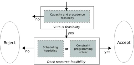
First, observe that, a necessary condition for an insertion to be feasible in the VRPCD-RC, is for it to be feasible in the VRPCD. As mentionned in Section 4.1.3, feasibility tests in the VRPCD can be performed in constant time. On the other hand feasibility test with respect to dock resource constraints in the VRPCD-RC cannot be done in constant time. Thus for maximal efficiency, we test the feasibility of an insertion as shown on Fig. 2: we start by checking if it is feasible for the VRPCD, if the insertion passes these tests, we test it with respect to dock resource constraints using either a CP solver or scheduling heuristics.
5.2. LNS operators
In the proposed LNS, we use the destruction operators of LNS+SPM (see Section 4.1.1). For repair operators, two facts should be taken into account: first, because of resource constraints, only a limited number of requests will be transferred (some requests that were transferred in the VRPCD may not be transferred in the VRPCD-RC). Thus, there is an incentive in creating routes without transfer. Second, as mentioned in Section 5.1.2, feasibility tests can no longer be performed in constant time, thus repair methods that check many insertions, such as k-regret with a high value of k, should be avoided. As such we use: best insertion, 2-regret, best insertion without transfer and 2-regret without transfer as repair methods. In the variants
Figure 2: Logical flow-chart of feasibility tests for the VRPCD-RC
5.3. Integration of dock resource constraints in the periodical set partitioning based problem
For the VRPCD-RC, adding dock resource constraints makes the SPM (see Section 4.2) significantly more difficult. Indeed preliminary tests showed that, very often, the CP solver could not find any solution to the corresponding matching and scheduling problem within reasonable runtimes. On the other hand we noticed that the scheduling problems of Section 5.1.1 were solved by the CP solver within a relatively small time. Thus, because the set partitioning idea proved very efficient in [? ], and to cope with the added complexity of the dock resource constraints, in place of SPM we propose to solve a Set Partitioning and Scheduling problem (SPS). It provides the best possible solution from a set of routes (instead of legs in the SPM). It is solved using branch-and-check. To that end a set partitioning problem on routes (similar to the SPP on legs of Section 4.2.2) is solved in a branch-and-bound fashion. At each integral node, the associated scheduling problem corresponds to the one in Section 5.1.1.
This approach is efficient to select the best routes but the matching of legs in these routes may be improved. At the end of the SPS, we solve an optimization version of the matching and scheduling problem of Section 4.2.2, where the objective is to minimize the volume transferred at the cross-dock. In the shared case, the CP problem is: min X (l,l0)∈ ˜L p× ˜Ld o−ll0.IsP resent × X r∈R− l,l0 qr (30) (10 - 20) X l∈Lp isActive(tl, h) ≤ I ∀h ∈ [0, H] (31) X l0∈L d isActive(t0l, h) ≤ O ∀h ∈ [0, H] (32)
(30) minimizes the volume transferred at the cross-dock, while constraints (31) and (32) account for the capacity constraints and are similar to (27) and (28) of Section 5.1.1. A similar problem for the separated case can be formulated with an adaptation of (29).
5.4. Structure of the proposed method
Algorithm 2 and Algorithm 3 present a sketch of the proposed method: LNS+SPS. Algorithm 2 is similar to Algorithm 1 except for two changes. First, since feasibility tests are computationally more intensive, we consider a stop-criterion based on time, and enclose all instructions within time conditions. Second, the pool of routes K (l. 2 in Algorithm 3) plays the exact same role as the pool of legs L in Algorithm 1. The pool of legs L is still present, it now acts as a memory that can help improving routes in K before solving the SPS, as presented in Algorithm 3. We first apply dominance rules to the legs in L (see Section 4.2). Then we try to improve each route in K by replacing its pickup leg and/or its delivery leg by a non dominated equivalent in L
(l. 2-4 in Algorithm 3). We remove dominated routes from K (l. 5 in Algorithm 3). A route is dominated iff there exists a route with a smaller cost that covers the same requests and can arrive earlier at the cross-dock and/or can leave later from the cross-dock. We solve the SPS, and eventually we try to improve the matching of legs in the solution. The initial solution is obtained by applying a 2-regret without transfer.
Result: The best found solution s?
1 Pool of legs L := ∅ 2 Pool of routes K := ∅
3 Generate an initial solution s 4 s?:= s
5 while stop-criterion not met do 6 s0:= s
7 Destroy quantity: select a number Φ of requests to remove from s0
8 Operator selection: select a destruction operator M− and a repair operator M+
9 Destruction : apply M− to remove Φ requests from s0, and put them in the requests bank of s0 10 Repair: apply M+ to reinsert the requests in the requests bank in s0
11 if acceptance criteria is met then 12 s := s0
13 end
14 if cost of s0 is better than cost of s? then 15 s?:= s0
16 end
17 Add legs of s0 to L 18 Add routes of s0 to R
19 if set partitioning and scheduling condition is met then 20 Perform SPS(L, K, s?, s0); 21 end 22 end 23 return s? Algorithm 2: LNS+SPS 6. Computational experiments
The algorithm is coded in C++ and uses CPLEX and CP Optimizer from IBM ILOG Cplex Optimization Studio 12.6.1 as MIP solver and CP solver, respectively. The experiments were conducted under Linux using an Intel Xeon X7350 @ 2.93 GHz. Only one core is used both by our code and third party solvers. We consider instances proposed by Wen et al [? ], that range from 50 to 200 requests. They are based on real life data from a Danish logistics company. The termination criterion for all algorithms is based on time: 15 minutes for size 50 instances, 30 minutes for size 100 for instances, 60 minutes for size 150 instances and 120 minutes for size 200 instances. SPS time limit is 180 seconds. These time limits are between two and three times the runtimes reported for the VRPCD in [? ]. As in [? ], the number Φ of requests to remove in the repair phase of the LNS is drawn randomly in the interval [min(30, 10% of |R|), max(60, 20% of |R|)], acceptance criterion is descent.
6.1. Bound setting for the number of docks
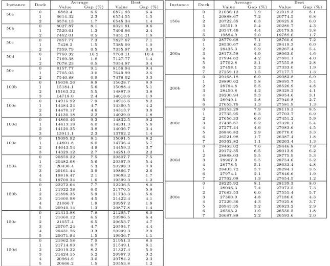
To determine when limiting the number of docks start being a constraint in the VRPCD-RC, we postpro-cessed the solutions obtained in [? ] for the VRPCD. To that end, for all the ten solutions found for each instance for the VRPCD, we solve optimization versions of the satisfaction scheduling problems introduced in Section 5.1.1. We take as objective: to minimize S in the shared case, and in the separated case, we only consider symmetric configurations where I = O and we minimize I. In table 1, columns A correspond to the smallest value obtained after two hours of runtime for the CP solver, and columns B correspond to the worst value obtained after five minutes of post-process. For each instance, columns B corresponds to a threshold for the dock value, above which, the VRPCD-RC could be solved as a VRPCD (postprocessing the solution for a
Input: pool of legs L, pool of routes K, solution s?, s0 from Algorithm 2
1 Remove dominated legs from L 2 for each route k ∈ K do
3 Replace, if possible, its pickup leg and/or its delivery leg with a non-dominated equivalent in L 4 end
5 Remove dominated routes from K 6 Solve SPS with all routes in K
7 if a new best solution has been found then
8 Improve the matching of legs (as in Section 5.3) 9 Update s?
10 end
11 if Set partitioning was not solved to proven optimality then 12 Clear K
13 end
Algorithm 3: Perform SPS
limited amount of time to satisfy dock resource constraints). As such, in our experiments for the VRPCD-RC, we will test dock values up to those reported in colums B.
From this table, we can observe that dock resource constraints arise for dock values that corresponds to approximately 15% of the fleet size in the shared case and 10% of the fleet size in the separated case.
Instance Avg. fleet size Separated Shared
A B A B 50a 14.2 2 2 2 2 50b 16.1 2 2 2 2 50c 16.0 2 2 2 3 50d 15.0 2 2 2 2 50e 16.0 2 2 2 3 100b 31.0 3 3 4 4 100c 31.5 3 3 4 4 100d 29.2 3 3 4 4 100e 32.0 3 3 4 5 150a 45.4 4 5 5 7 150b 46.9 4 5 6 7 150c 45.9 4 5 6 7 150d 45.0 4 5 6 7 150e 46.0 4 5 6 7 200a 62.9 6 7 8 9 200b 62.0 6 6 8 9 200c 61.1 6 7 8 9 200d 62.0 6 7 8 9 200e 62.0 6 7 8 10
Table 1: Dock value obtained when postprocessing for each instance all of ten solutions of [? ]. Columns A refer to the to the best solution (min dock use) obtained after two hours, while columns B correspond to the worst value (max dock use) obtained
after five minutes of post-processing.
6.2. Parameters tuning
In this section we evaluate and adjust several parameters. We start with the time limit for the CP solver in LNS feasibility tests, then we report the success rate of heuristics. After, we present the influence of the SPS frequency on the quality of solutions, and eventually we compare the performance of four possible configurations: with CP solver tests/with heuristic tests in LNS, with/without SPS. For tuning, we use instances 50b, 100b, 150b, 200b, and we consider the shared cross-dock configuration case.
6.2.1. CP solver time limit in feasibility tests
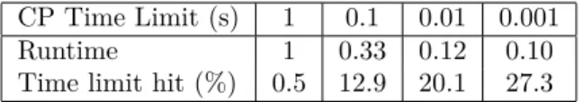
When checking the feasibility with respect to dock resource constraints, we need to set a time limit after which the CP solver will stop searching and declare the insertion infeasible. This avoids spending a large amount of time checking the feasibility of a single insertion. In Table 2, we compare four different time limits. In the final setting, the time limit of the CP Solver is set to 0.01 seconds
6.2.2. Heuristics performance
As mentioned in Section 5.1.2, using CP versus using heuristics for feasibility tests is a quality/runtime trade-off. For each instance in the training set, we performed two runs with LNS, with the stop-criterion
CP Time Limit (s) 1 0.1 0.01 0.001
Runtime 1 0.33 0.12 0.10
Time limit hit (%) 0.5 12.9 20.1 27.3
Table 2: Comparison of four different time limits for the CP solver, when used as feasibility test in the shared case. Runtime is normalized with 1 representing the runtime for a CP solver time limit of 1s. Time limit hit represents the percentage of calls for which the CP solver could not find an answer within the time limit. Figures reported for one thousand LNS iterations, two runs
were performed in each case.
set to one thousand iterations. We count how many time insertions were reported feasible by heuristics and how many times they were reported feasible by the CP solver with a time limit of 1 second (according to Table 2, with this time limit we can consider that the CP solver give an accurate answer most of the time). On average, 71.1% of feasible insertions are reported feasible by heuristics. Performing one thousand LNS iterations with feasibility tests performed by heuristics takes only 18.2% of the time taken with CP solver tests (with 0.01s as time limit).
6.2.3. SPS frequency
In [? ], the SPM was solved twenty times per run (every thousand iterations with a stop-criterion of twenty thousands iterations). In the VRPCD-RC, because feasibility tests are computationally intensive, the stop-criterion is based on time. The number of iterations performed within the time limit depends not only on the size of the instance but also on the dock value. As such, we propose a SPS-criterion based on time. In Table 3 and Table 4, we compare three different settings for the SPS frequency : 10, 20 and 40 calls within the time limit. Accordingly, the number of calls per run is set to 20 for heuristic test and 10 for CP solver test.
Number of calls 10 20 40 Average gap (%) 0 -0.70 -0.29
Table 3: Comparison of the impact of the number of SPS calls per run on the quality of the solution for heuristic feasibility tests. Five runs were performed for each dock value for each instance in the training set. 10 calls is taken as reference for the gap
Number of calls 10 20 40 Average gap (%) 0 +0.40 +0.68
Table 4: Comparison of the impact of the number of SPS calls per run on the quality of the solution for CP solver tests. Five runs were performed for each dock value for each instance in the training set. 10 calls is taken as reference for the gap
6.2.4. Performance comparison
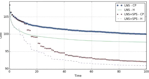
On Fig. 3 we present the convergence curves of LNS and LNS+SPS over time for both CP solver and heuristics feasibility tests. From this graph, we can observe two things. First, as in the VRPCD, periodically solving a set partitioning based problem significantly improves performance compared to LNS alone: -6.96% for heuristic test and -7.92% for CP solver test on average. Second, the best performing method is LNS+SPS with heuristic feasibility tests, as it finds solutions that are 1.19% better on average than LNS+SPS with CP solver test. In the rest, we thus use LNS+SPS with heuristic feasibility test.
6.3. Results
Table 5 and Table 6 present the results in the shared case and in the separated case respectively. A dock value of 0 corresponds to the case where no transfer is allowed. These results highlight the increased complexity induced by integrating dock resource constraints, as there exists for each instance, at maximum dock value, a solution with 0% gap (see Section 6.1). Nevertheless LNS+SPS finds solutions that are 1.6% more expensive in the shared case and 1.5% more expensive in the separated case, which remains satisfactory. The algorithm shows relatively good performance in terms of stability: the difference between the average value and the best value of the five runs for each instance and each dock value is 0.6% on average and at most 1.4% in the shared case and 0.6% on average and at most 3.2% in the separated case.
Figure 3: Comparison of the evolution of the average solution quality over time (in percentage of time limit) for four different configurations: with CP solver/with heuristics tests, with/without SPS. The results aggregate 5 runs for each dock value in the shared case for instances in the training set. They have been normalized, first by instance then by method, with 100 representing
the cost at the end of LNS with CP solver tests (LNS-CP)
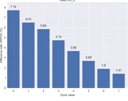
Regarding routing costs: integrating dock resource constraints implies an increase in cost. Comparing the two systems, the shared case costs are slightly smaller than separated costs (e.g, for instance 150b, 5.85% for 2 shared docks compared to 6.05 as shown on Fig. 4). This differences increases with the number of docks.
7. Conclusion
This paper presents an adaptation of the method proposed in [? ], which is based on large neighborhood search and periodic calls to a set partitioning based problem, to solve an extension of the VRPCD that includes resource synchronization constraints at the cross-dock. To deal with these constraints, scheduling heuristics and a CP model have been used as feasibility tests for insertions in LNS. In this case, experiments have showed that heuristics are the most efficient compromise. Compared to [? ], because of the increased complexity induced by resource synchronization constraints, the set partitioning based problem had to be adapted with a simpler subproblem. As in [? ], adding this component helps finding solutions significantly better than those obtained by LNS alone. The proposed method has been tested on instances from the literature, where it shows an increase in routing costs with the decrease in cross-dock capacity.
Instance Dock Average Best Value Gap (%) Value Gap (%) 50a 01 6682.726882.4 6.53.4 6871.936628.05 6.42.7 2 6530.81 1.0 6471.48 0.2 50b 0 8027.87 8.1 8021.81 9.6 1 7609.07 2.4 7541.33 3.0 2 7481.99 0.7 7470.78 2.0 50c 01 7857.777505.34 7.32.5 7827.677473.94 7.12.2 2 7449.88 1.8 7397.38 1.2 3 7338.88 0.3 7330.08 0.3 50d 0 7760.32 10.2 7760.11 10.4 1 7272.57 3.3 7206.48 2.5 2 7108.91 1.0 7076.13 0.7 50e 0 8157.77 9.1 8156.94 9.4 1 7843.08 4.9 7772.39 4.3 2 7616.54 1.8 7554.75 1.4 3 7537.85 0.8 7473.56 0.3 100b 0 15636.26 8.8 15628.7 8.9 1 15322.86 6.6 15234.2 6.2 2 15181.04 5.6 15073.8 5.0 3 14929.18 3.8 14810.3 3.2 4 14700.96 2.3 14620.3 1.9 100c 0 14915.92 7.9 14915.6 8.2 1 14654.16 6.0 14611.5 6.0 2 14456.6 4.5 14395.0 4.4 3 14353.9 3.8 14188.2 2.9 4 14145.78 2.3 14081.3 2.2 100d 0 14860.46 9.3 14832.5 9.2 1 14424.74 6.1 14338.9 5.6 2 14316.7 5.3 14207.4 4.6 3 14070.18 3.5 13976.2 2.9 4 13866.24 2.0 13774.7 1.5 100e 0 15095.92 8.1 15091.5 8.2 1 14819.26 6.2 14733.8 5.7 2 14783.82 5.9 14622.8 4.9 3 14515.0 4.0 14384.7 3.2 4 14357.26 2.9 14258.4 2.3 5 14281.0 2.3 14085.3 1.0 150a 0 20859.22 7.5 20807.7 7.5 1 20534.8 5.8 20406.4 5.4 2 20505.68 5.7 20342.5 5.1 3 20248.54 4.4 20090.1 3.8 4 20110.14 3.7 19988.6 3.3 5 19822.08 2.2 19740.0 2.0 6 19725.04 1.7 19629.7 1.4 7 19603.78 1.0 19541.6 0.9 150b 0 22272.64 7.7 22236.5 8.0 1 22018.68 6.5 21934.5 6.6 2 21882.36 5.9 21825.0 6.0 3 21651.48 4.7 21585.3 4.9 4 21432.16 3.7 21360.2 3.8 5 21227.66 2.7 21097.6 2.5 6 21065.9 1.9 20986.2 2.0 7 20963.44 1.4 20899.9 1.5 150c 0 21313.88 7.8 21295.7 8.0 1 21095.74 6.7 20959.6 6.2 2 20945.68 5.9 20854.4 5.7 3 20869.2 5.5 20642.1 4.6 4 20685.7 4.6 20559.7 4.2 5 20475.68 3.6 20369.1 3.3 6 20208.76 2.2 20155.8 2.2 7 20153.68 1.9 20100.9 1.9 150d 0 21962.58 7.9 21951.3 8.0 1 21735.46 6.8 21536.0 6.0 2 21609.34 6.2 21442.6 5.5 3 21448.08 5.4 21368.0 5.2 4 21504.76 5.6 21289.8 4.8 5 21040.52 3.4 20874.7 2.7 6 20806.38 2.2 20642.2 1.6 7 20715.78 1.8 20608.5 1.4
Instance Dock Average Best
Value Gap (%) Value Gap (%)
150e 0 21036.12 7.9 21019.3 8.1 1 20827.96 6.8 20703.5 6.4 2 20774.68 6.6 20587.3 5.9 3 20599.16 5.7 20320.2 4.5 4 20398.18 4.6 20341.0 4.6 5 20346.68 4.4 20245.7 4.1 6 20073.92 3.0 20025.5 3.0 7 19915.4 2.2 19773.1 1.7 200a 0 28779.68 7.1 28760.6 7.2 1 28507.12 6.1 28423.1 6.0 2 28516.14 6.2 28263.0 5.4 3 28273.0 5.2 28159.1 5.0 4 28323.38 5.4 28146.5 5.0 5 28151.24 4.8 28054.8 4.6 6 28099.32 4.6 27959.8 4.3 7 27922.8 3.9 27782.5 3.6 8 27704.08 3.1 27527.8 2.7 9 27497.36 2.4 27391.5 2.1 200b 0 29168.18 6.9 29082.8 6.9 1 28962.52 6.1 28771.7 5.7 2 28809.76 5.5 28751.4 5.6 3 28784.88 5.5 28514.1 4.8 4 28589.7 4.7 28546.4 4.9 5 28374.36 4.0 28186.6 3.6 6 28446.44 4.2 28234.3 3.7 7 28156.7 3.2 28091.2 3.2 8 27889.54 2.2 27677.2 1.7 9 27630.92 1.2 27516.8 1.1 200c 0 28153.28 7.9 28119.3 8.5 1 27996.14 7.3 27819.7 7.3 2 27744.12 6.4 27555.7 6.3 3 27629.96 5.9 27381.3 5.6 4 27534.98 5.5 27207.7 4.9 5 27522.48 5.5 27315.8 5.4 6 27236.38 4.4 27135.5 4.7 7 26921.14 3.2 26820.2 3.4 8 26685.4 2.3 26570.1 2.5 9 26583.44 1.9 26477.1 2.1 200d 0 29463.02 7.6 29446.8 7.8 1 29328.88 7.1 29227.0 6.9 2 29126.9 6.3 28993.7 6.1 3 28962.52 5.7 28825.7 5.5 4 28866.58 5.4 28776.3 5.3 5 28777.12 5.0 28523.2 4.4 6 28708.02 4.8 28546.4 4.5 7 28467.38 3.9 28283.7 3.5 8 28208.72 3.0 28129.6 2.9 9 28002.7 2.2 27877.6 2.0 200e 0 28225.92 8.1 28139.3 8.0 1 28106.28 7.7 28001.5 7.4 2 27935.84 7.0 27659.2 6.1 3 27789.42 6.4 27566.0 5.8 4 27610.22 5.8 27432.2 5.3 5 27421.46 5.0 27113.3 4.0 6 27324.54 4.7 27067.2 3.9 7 27061.8 3.7 26967.5 3.5 8 26858.48 2.9 26772.0 2.7 9 26665.24 2.1 26543.9 1.8 10 26677.62 2.2 26600.4 2.1
Table 5: Average values and best solution found in the shared cross-dock configuration case; LNS+SPS was run five times for each instance. Columns Gap refer to the gap to average values and best solutions reported in [? ] for the VRPCD
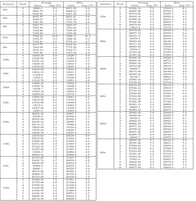
Instance Dock ValueAverageGap (%) Value BestGap (%) 50a 0 6882.4 6.5 6871.93 6.4 1 6614.32 2.3 6554.55 1.5 2 6574.13 1.7 6545.34 1.4 50b 01 8027.877520.61 8.11.3 8021.817496.96 9.62.4 2 7462.01 0.5 7451.21 1.8 50c 0 7857.77 7.3 7827.67 7.1 1 7428.2 1.5 7385.09 1.0 2 7359.79 0.5 7335.97 0.3 50d 01 7760.327169.38 10.21.8 7760.117127.77 10.41.4 2 7078.23 0.5 7054.87 0.4 50e 0 8157.77 9.1 8156.94 9.4 1 7705.03 3.0 7649.99 2.6 2 7546.88 0.9 7478.02 0.3 100b 0 15636.26 8.8 15628.7 8.9 1 15184.1 5.6 15088.4 5.1 2 15163.32 5.5 14887.9 3.8 3 14718.0 2.4 14618.6 1.9 100c 0 14915.92 7.9 14915.6 8.2 1 14484.24 4.7 14360.5 4.2 2 14470.17 4.6 14313.7 3.8 3 14130.18 2.2 14029.0 1.8 100d 0 14860.46 9.3 14832.5 9.2 1 14413.18 6.0 14331.3 5.6 2 14120.35 3.8 14036.7 3.4 3 13911.1 2.3 13762.2 1.4 100e 0 15095.92 8.1 15091.5 8.2 1 14801.8 6.0 14736.4 5.7 2 14643.54 4.9 14459.3 3.7 3 14329.12 2.7 14251.0 2.2 150a 0 20859.22 7.5 20807.7 7.5 1 20482.68 5.6 20397.9 5.4 2 20430.4 5.3 20298.3 4.9 3 20161.44 3.9 19866.7 2.6 4 19818.47 2.1 19683.2 1.7 5 19709.34 1.6 19599.3 1.2 150b 0 22272.64 7.7 22236.5 8.0 1 21922.38 6.0 21770.5 5.8 2 21896.35 5.9 21733.3 5.6 3 21600.98 4.5 21422.4 4.1 4 21060.7 1.9 20957.2 1.8 5 20940.14 1.3 20877.8 1.4 150c 0 21313.88 7.8 21295.7 8.0 1 21060.12 6.5 20986.5 6.4 2 21057.4 6.5 20653.7 4.7 3 20707.24 4.7 20594.7 4.4 4 20431.26 3.3 20299.3 2.9 5 20071.94 1.5 19936.7 1.1 150d 0 21962.58 7.9 21951.3 8.0 1 21714.83 6.7 21549.1 6.1 2 22019.32 8.2 21327.4 5.0 3 21424.15 5.2 20967.3 3.2 4 20964.9 3.0 20784.2 2.3 5 20666.2 1.5 20553.8 1.2
Instance Dock ValueAverageGap (%) Value BestGap (%)
150e 0 21036.12 7.9 21019.3 8.1 1 20888.67 7.2 20774.5 6.8 2 20722.35 6.3 20625.8 6.0 3 20551.0 5.4 20280.7 4.3 4 20347.46 4.4 20179.9 3.8 5 19884.9 2.0 19789.0 1.7 200a 0 28779.68 7.1 28760.6 7.2 1 28530.67 6.2 28419.3 6.0 2 28435.3 5.9 28267.4 5.4 3 28173.58 4.9 28063.0 4.6 4 27994.62 4.2 27881.1 4.0 5 27702.8 3.1 27555.8 2.8 6 27458.1 2.2 27333.0 1.9 7 27259.12 1.5 27177.7 1.3 200b 0 29168.18 6.9 29082.8 6.9 1 28890.62 5.8 28695.7 5.4 2 28784.8 5.5 28526.9 4.8 3 28450.8 4.2 28329.2 4.1 4 28200.94 3.3 28054.6 3.1 5 28049.1 2.8 27940.8 2.7 6 27653.76 1.3 27581.9 1.3 200c 0 28153.28 7.9 28119.3 8.5 1 27735.95 6.3 27703.7 6.9 2 27656.33 6.0 27451.2 5.9 3 27435.67 5.2 27320.1 5.4 4 27277.44 4.6 27083.6 4.5 5 26846.82 2.9 26776.0 3.3 6 26521.98 1.7 26387.4 1.8 7 26362.82 1.1 26263.4 1.3 200d 0 29463.02 7.6 29446.8 7.8 1 29172.35 6.5 29013.9 6.2 2 28888.03 5.5 28775.9 5.3 3 28907.9 5.5 28754.6 5.2 4 28778.5 5.1 28633.4 4.8 5 28403.72 3.7 28294.1 3.5 6 27974.1 2.1 27846.6 1.9 7 27762.08 1.3 27654.5 1.2 200e 0 28225.92 8.1 28139.3 8.0 1 28046.3 7.4 27972.5 7.3 2 27683.53 6.0 27555.4 5.7 3 27360.9 4.8 27186.0 4.3 4 27229.36 4.3 27025.6 3.7 5 26943.35 3.2 26823.2 2.9 6 26593.2 1.9 26530.5 1.8 7 26687.88 2.2 26593.6 2.0
Table 6: Average values and best solution found in the separated cross-dock configuration case; LNS+SPS was run five times for each instance. Columns Gap refer to the gap to average values and best solutions reported in [? ] for the VRPCD
(a) Shared cross-dock configuration
(b) Separated cross-dock configuration
Figure 4: Influence of the dock value for instance 150b. Five runs were performed for each dock value. The y-axis represents the average gap with respect to the average value reported in [? ]
![Table 1: Dock value obtained when postprocessing for each instance all of ten solutions of [? ]](https://thumb-eu.123doks.com/thumbv2/123doknet/12202566.316128/13.918.334.583.499.690/table-dock-value-obtained-postprocessing-instance-solutions.webp)