Validation of the Large Eddy Simulation model in building

(1)

1

Validation of the Large Eddy Simulation model in building

physics

Barbason Mathieu

1

*, Reiter Sigrid

1

(1) _{Université de Liège, Belgique}

1. ABSTRACT

Environmental concerns and growing computer resources have promoted the emergence of new simulation tools and especially Computational Fluid Dynamics (CFD). Turbulence modelling is a key for a good simulation. Unfortunately, models are numerous: Reynolds-Averaged Navier-Stokes (RANS), Detached Eddy Simulation (DES), Large Eddy Simulation (LES), etc. Moreover, there are lots of physical phenomena involved in building physics. Consequently, it is often difficult for a non-expert user to choose efficiently their models. This paper describes results obtained with LES for three different cases. These cases were retained to represent the most common situations encounter in building physics. Results are good and so the use of LES is validated for building physics simulations. RANS and DES results are also introduced to have a global view of the capacity of CFD simulations. RANS results are sufficient for the most current applications in building physics. But LES and DES can improve the results and give complementary data.

Keywords: Building Physics Simulations, CFD, Validation, LES 2. INTRODUCTION

Energy consumption has become one of the biggest stakes of this decade. For this reason, the scientific community is urged to make energy save in every area. As a large part of energy consumption is due to buildings, innovative solutions are needed. With improving computer capacities, new tools appear. Computational Fluid Dynamics (CFD) is one of them. Originally developed for aerospace applications, it is now getting mature for building physics simulations. In the future, it will help architects and building engineers to better understand physical phenomena and to improve drastically Heating, Ventilation and Air-Conditioning (HVAC) systems efficiency and Internal Air Quality (IAQ).

Physical phenomena encountered in building physics are numerous and require different approaches. For example, turbulence modelling is very tricky as there are different techniques. The quality of the results depends strongly on the choice of the operator and, unfortunately, there is no clearly defined method to help non-expert users to get used to CFD techniques. This paper is intended to compare different turbulence modelling approaches to help new users to make the good choice in function of their expectations.

This paper is written in the frame of an EDRF project called SIMBA. The aim of this project is to validate various CFD simulation tools, and to confront CFD and multizonal approaches.

3. COMPUTATIONAL FLUID DYNAMICS

CFD is more and more used in building physics because it permits to have a very precise description of the airflow in thousands of points inside each room. Thanks to CFD, we can expect a lot of improvements in air quality and occupant’s thermal comfort. For example, Méndez et al. (2008) have studied the air quality inside a hospital room to ensure the best air quality in function of the position of the mechanical ventilation. It has proved that the initial

(2)

2

architectural design was not good and that it is possible to improve drastically the air quality near patients. Papakonstantinou et al. (2000) have studied the airflows inside an archaeological museum in Athens where it is also crucial to ensure a good thermal environment both for occupants and for the museum pieces. Hu et al. (2010) are studying the possibility to use CFD in fire cases to help rescuer to determine the origin of the fire and its progression during their work.

Unfortunately, the modelling of a flow becomes complex when the flow becomes turbulent. Indeed, the flow is then characterized by a chaotic evolution. The mathematical description of the motion of a fluid entity becomes very complex and different approaches have emerged. Generally, the flow prediction is done by three approaches: Direct Numerical Simulation (DNS), Large-Eddy Simulation (LES) and Reynolds Averaged Navier-Stokes (RANS) simulation (Lampitella, 2009).

3.1 Direct Numerical Simulation

With this technique, the Navier Stokes equations are resolved without assumption on a very fine spatial mesh and a very small time step. Thus, this technique, applied to building physics, requires numerical capacities that are far beyond computer capacities.

3.2 Large-Eddy Simulation

Turbulent motion can be separated into two parts: large eddies and small eddies. The first ones are anisotropic and so need to be resolved in details while the second ones are isotropic and can be modelled. The distinction is done through the mesh refinement. This technique is known to work well far away from walls which can be problematic for internal airflows. 3.3 Reynolds-Averaged Navier-Stokes Simulation

This technique does not make the difference between large and small eddies. Every turbulent phenomenon is modelled. Of course, it is an important assumption but it permits to gain a lot of computing time and numerical resources. Wall treatment can also be a problem depending on the model.

It should be noted that there is a technique called Detached Eddy Simulation (DES) that permits to use LES faraway from walls and RANS simulation near walls.

This paper will focus on the LES technique that is supposed to give better results. It will permit to assess the reliability of CFD techniques thanks to experimental results. Moreover, RANS and DES results are also provided to show a global view of CFD capacities. Indeed, it is interesting to compare the results to understand how to make the best choice for the turbulence model.

Note that there are lots of studies about this topic because the turbulence modelling is very complex. For example, Voigt (2000) and Kuznik et al. (2007) have compared several RANS techniques. More recently, Wang and Chen (2010) have also compared RANS, DES and LES techniques.

4. CASE DESCRIPTION

As this paper is intended to help building designers and architects, three of the most common cases were identified and developed: a natural convection case, a mixed convection case and a natural ventilation case. Indeed, the first one corresponds to the simplest case with only thermal loads inside a room. These thermal loads can be imposed by a heat flux (and so represents for example a radiator or a computer) or by an imposed temperature on a wall (for

(3)

3

a heating wall or a cooling ceiling for example). The second case corresponds to mechanical ventilation. This type of device implies a forced convection that, coupled with thermal loads, becomes a mixed convection case. Eventually, the third case deals with natural ventilation that appears more and more as the easiest way to improve occupant’s thermal comfort while saving energy consumptions.

With this panel of cases, three systems for improving air quality and occupant’s thermal comfort are tackled: radiant panel, mechanical ventilation and natural ventilation.

As said before, this paper is intended to provide a holistic approach for non-expert users to judge their CFD results. Chen and Srebric (2001) have elaborated a procedure to compare experimental and numerical data to validate the use of a CFD code in a specific case. This paper will scrupulously follow this procedure. Note that in their paper, Chen and Srebric (2001) developed a mixed convection case as example of their validation procedure.

Chen and Srebric (2001) described a three step validation (verification, validation and results report). The first step aims to verify that the code is able to model the physical phenomena involved in the studied case, the second step validate the code for mixed case and the ability of the user. The third step imposes to report the results in a precise way. As the first step is mainly intended for code developers, this article only considers the two last steps.

In the following, each case will first be introduced. The result section will be devoted to the detailed description of the results obtained with a well established commercial CFD code. The comparison with experimental data will validate the use of this software for building physics simulations.

4.1 Case 1: Natural Convection Case

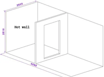
Radiant panels are more and more used in buildings and the aim of this case is to make the operator able to describe correctly this type of installation. The experimental data comes from a study of the University of Liège led by Tang (1998). The test room is composed of two parts separated by an opening (see Figure 1). The only heating device is a heating wall in the smallest part. Wall temperatures are imposed on every wall.

(4)

4 4.2 Case 2: Mixed Convection Case

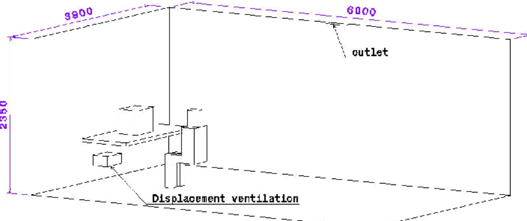
This case is a displacement ventilation with thermal loads that interact directly with the jet. Indeed, the air inlet is directed on a simulated person (see Figure 2). The experimental data comes from a study of Yang et al. (2007). It will be interesting to see if the CFD software can take into account mixed convection. Moreover, thanks to this case, the operator gets used to body simulation.

4.3 Case 3: Natural Ventilation Case

This case was first studied by Jiang and Chen (2003). There are two types of natural ventilation: buoyancy-driven and wind-driven ventilation (Jiang et al., 2004). Only the first case was retained because it is the most difficult to model, due to smaller pressure differences. Buoyancy-driven ventilation is also the most interesting case in temperate climate. Indeed, the “worst scenario” that could happen is a warm and windless day (Jiang and Chen, 2003). This case is a room inside a bigger one which reproduces external conditions (see Figure 3).

Figure 2. Illustrations of the mixed convection case (Yang et al., 2007).

a) b)

(5)

5

5. DISCUSSION AND RESULTS ANALYSIS

In this section, a widely used software in CFD is submitted to the three cases. These case are deeply analyzed in accordance with Chen and Srebric (2001).

5.1 Case 1: Natural Convection Case

5.1.1 Geometrical description

This case is a two zones case. A heating wall is placed inside the smallest room. The two rooms are separated by a 2.06m x 1.25m opening. The complete plan of this case is given in Tang and Robberechts (1989).

5.1.2 Experiment description

Three poles with five air temperature and velocity sensors were placed in each room to measure air temperatures. Results will be given for the two room-centered columns. The air temperature and velocity is also monitored in the opening by several sensors. Note also that wall temperatures are monitored which will permit to define precisely boundary conditions.

5.1.3 Turbulence model

For LES study, the main choice concerns the modelling of the subgrid scale phenomena. the CFD software proposes three different approaches and a WALE model (Nicoud and Ducros, 1999) was chosen because it takes into account the impact of walls.

Concerning the RANS modelling, a SST k-ω model was chosen (Menter, 1994) because it gives satisfactory results (Barbason and Reiter, 2010).

5.1.4 Boundary conditions

Boundary conditions are quite simple. The only two hypotheses are a uniform wall temperature on each wall and a no-slip condition. Values for temperatures are given in Tang (1998).

5.1.5 Numerical methods

The Navier-Stokes equations were discretized by a finite volume method with a cell-based approach. For the velocity-pressure coupling, the SIMPLEC numerical algorithm was used. The derivatives were discretized with a QUICK scheme. To ensure the best convergence, the technique of Cook and Lomas (1997) was used (combination of under-relaxation and false time-stepping). Solution was considered as converged when no further change was noticed in the solution during one hundred iterations.

Meshes were different for the two turbulence models. Indeed, each model has its own characteristics. LES requires a much more fine mesh (2 100 000 cells) than the RANS model (400 000 cells). It has important repercussions on computing time. For the two cases, mesh is composed of tetrahedral cells.

5.1.6 Results

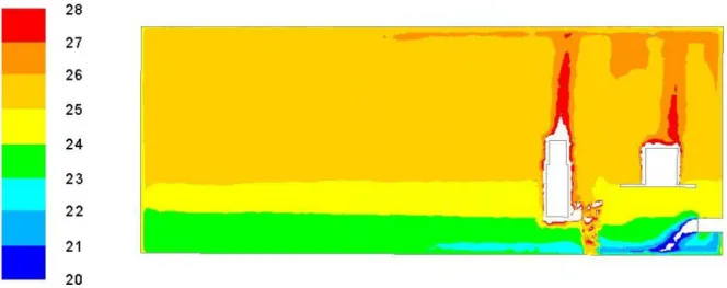
Chen and Srebric (2001) suggest beginning the presentation of the results with a global analysis of the numerical results. It only aims to check that the solution is physically possible. The simplest way to achieve this is to check the results for air temperature or air velocity in a zone of interest. For example, for the natural convection case, Figure 4 illustrates the air

(6)

6

temperature in the central plane. It clear proves that there is one convection cell which straddles the two rooms.

Figure 4: Air Temperature in the Median Plane.

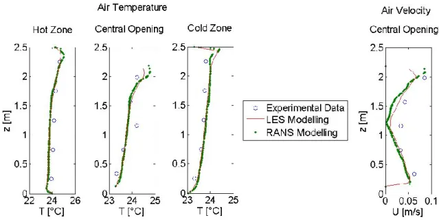
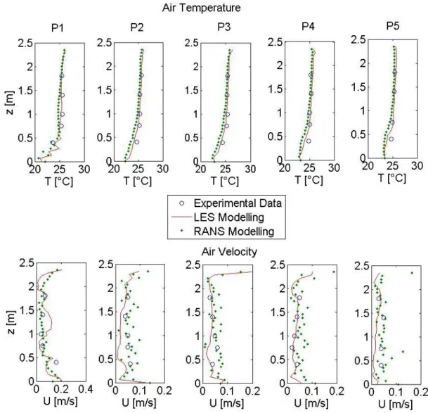
The second step of the validation phase is to compare numerically and graphically the primary variables (air temperature and velocity, air exchange rate, etc.). Results for air temperature and velocity are given at Figure 5.

(7)

7

First of all, it is important to underline that there is hardly any difference between LES and RANS simulations except near wall. This is logical because near wall treatment is different: k-ω RANS simulations use a low-Reynolds correction to model the behaviour close to walls while LES requires mesh refinement near walls to calculate every phenomenon occurring. Of course, this implies much more computing time and resources.

There is a quite good agreement between experimental and numerical results, especially for air temperature. Small air velocities are not well described but it is probably due to the difficulty to obtain accurate results experimentally in this case. Despite this, the mean difference between numerical and experimental results on air velocity is less than 0.02m/s. This result is of course very good. Concerning air temperature, the mean difference is about 0.2°C which is once again very good.

It should be noted also that gradients of temperature are also well captured. The only bad result concerns the third sensor of the central opening but it is probably due to an experimental deficiency.

The third step of the reporting phase described by Chen and Srebric is to analyze results for the secondary variables (turbulent kinetic energy spectra for example). This third point will not be investigated for these three cases because it would go beyond the scope of this research. Moreover, it would imply much more computing time.

5.1.7 Conclusions

Results are very good and prove the ability of CFD to model correctly natural convection inside a room with a LES approach. This result is fundamental because natural convection occurs in every real case. Indeed, thermal loads can be numerous (human person, computer, lighting, radiator, wall heating, etc.). This heating wall case is also very interesting because radiant surfaces are more and more used in new buildings.

The agreement of the results is very good; the mean error is inferior to the precision of the equipment. This is also due to the simplicity of the case. The mean error is inferior to 5% of the range. It would have been interesting to have the mass flow rate through the opening to compare our results. Indeed, this value is a very important variable to evaluate air quality. 5.2 Case 2: Mixed Convection Case

This case is a single room equipped with a displacement ventilation. There is a human simulator sat in front of a computer. This case is very close to a real situation. The dimensions of the supply diffuser are 0.4m (length) x 0.15m (width) and the air supply rate is 43m³/h (0.79 Air Changes per Hour). The dimensions of the outlet diffuser are 0.34m x 0.14m. The air is injected with a temperature of 19°C. It should be noted that there is no other obstacles inside the room and that the outlet is in the ceiling. The complete plan of the case is given in Yang et al. (2007).

This paper focuses on the distribution of air temperature and air velocity inside the room. Experimental data were obtained by five poles placed in the median plane and around the body. The position of the poles is described in Figure 6.

(8)

8

Figure 6: Experimental Poles Positions (Yang et al., 2007).

24 probes were placed on the poles at different height (0.4, 0.75, 1, 1.4 and 1.8m). The probes sampled data every 30 seconds in 30 minutes

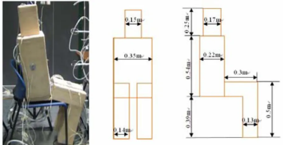
Concerning the body, the simulator is 1.6m height and the surface area is 1.68m² (mean value for a human body). A description of the human simulator is given at figure 4. Heating panels are placed inside the body and deliver 76W (typical value for a sat person). Eventually, the computer power is simulated by a lamp placed inside a box. The heat generated by this device is fixed to 40W.

Figure 7: Human simulator description (Yang et al., 2007).

As for the previous case, a SST k-ω model was used for RANS simulation. It should be noted that k-ω model has the advantage to simplify drastically near-wall treatment compared to a k-ε model. Indeed, it does not need any wall function thanks to a low-Reynolds correction.

(9)

9

The subgrid scale model for LES was a WALE model for the same reason as before.

Walls temperatures are supposed uniform and values for each wall are given in Yang et al. (2007). The temperature of the human body is not imposed but a constant heat flux is imposed (76W) equally distributed on the body surface. This hypothesis is not ideal because in the experimental case, the main part of the flux is emitted in the chest part (where the lamp is) and not in the legs. The error made by this approximation is supposed to be small. Concerning the computer, a constant flux of 40W is imposed on the whole surface.

The air velocity through the inlet is supposed to be uniform. This is also false but the approximation is supposed to have repercussions only near the inlet. The outlet is model by a uniform pressure distribution.

Concerning the discretization and convergence criterion, the parameters of the natural convection case were used.

As for the first case, meshes are different for the two modelling case: 1 050 000 tetrahedral cells for LES and 400 000 tetrahedral cells for RANS simulation. Mesh size were chosen such as results do not change if mesh size is increased.

5.2.6 Results

Figure 8 shows the air temperature repartition. It can be deduced from this image that there is two phenomena occurring: the natural convection due to the thermal loads (body and computer) and the forced convection due to the displacement ventilation. It will be interesting to see if CFD software can accurately model mixed convection. At first sight, it is possible to see that the upper part of the room is dominated by the natural convection cell and the bottom part is driven by the forced convection. This repartition is logical.

Figure 8: Air Temperature in the Median Plane.

It is interesting to focus on the zone between the legs of the simulated body. This zone is very hot due to the proximity of the two heated surface. Phenomena are probably strongly unstable and gradients important. It is not surprising to see that CFD software has some difficulty to

(10)

10

converge to a smooth solution. This phenomenon is also visible at Figure 9 (Pole P1) for the first column: results for air temperature and velocity are varying strongly.

The agreement between experimental and numerical data is also very good. The only problem concerns air velocity with RANS modelling. Indeed, the mean magnitude is good but results vary very quickly. The mean air temperature error is 0.25°C which is once very good given the range of temperature inside the room (8°C – 3% of error) for both RANS and LES. Concerning the air velocity error, the mean error is about 0.02m/s with both models. It proves that the mean magnitude found with the RANS technique is good.

Figure 9: Results of the Mixed Convection Case.

It is interesting to analyse the error on air temperature even if it is very small. The main part of the error is done in the inferior part (dominated by the forced convection). There are two explanations to this: the difficulty to correctly model a jet and the near-wall treatment. The first problem is inherent to CFD modelling and will probably last for a long time. Of course, this means that the operator needs experience while dealing with mechanical ventilation. Near-wall treatment is important and requires undoubtedly experience from the operator. There is no miracle solution and mesh refinement near wall implies more computing time and resources. A mid-way solution between LES and RANS modelling is to use DES.

(11)

11

This example proves the ability of CFD software to correctly model mixed convection. This case is more complicated than simply natural convection but it is possible to keep the mean error on air temperature below 5% of the range. Concerning air velocity, the prediction is good with an uncertainty of about 0.02m/s. With these two variables correctly described, it is possible to predict with accuracy occupant’s thermal comfort.

This case is very interesting because it shows that air temperature and velocity can be predicted very precisely in the vicinity of a human body and so comfort variables (Predicted Mean Vote – PMV – and Predicted Percentage Dissatisfied – PPD). It is also the occasion for the operator to get used to real situation because it is a typical office.

5.3 Case 3: Natural Ventilation Case

This case is a two rooms case. The experimental chamber is surrounded by a greater room that simulates external conditions. The two rooms are connected by an opened window measuring 0.90m x 0.99m. Note also that there is a 1500W baseboard heater inside the experimental chamber to intensify the natural convection.

Four poles were placed inside the experimental chamber in accordance with Figure 10. On each pole there are five air temperature and velocity sensors. One pole is also placed outside the experimental chamber but only poles P2 to P5 will be used in the followings. Indeed, the domain of interest is the experimental chamber.

Figure 10: Experimental Poles Positions (2003).

A RANS SST k-ω model is used for the same reason as before.

On the other hand, for the LES model, it was decided to innovate and to switch to a DES model. Indeed, in the paper of Jiang and Chen (2003), it is already proven that LES can accurately describe this case. So it is interesting to introduce DES modelling and its advantages. The aim of DES model is to conjugate RANS strength (calculation speed, near-wall treatment, etc.) and LES advantages (precision, turbulence modelling, etc.).

(12)

12

The model is constructed on the following principle: a RANS technique is used near wall while outside this zone, a LES technique is applied. Near-wall treatment is easier with RANS simulations and especially with a k-ω model thanks to the low-Reynolds correction. Moreover, the most complex and the smallest turbulent cells (which are close to the wall) are now taken into account by the RANS technique. This permits to increase the mesh and the time step and to keep LES everywhere else.

Walls of the experimental chamber are supposed adiabatic while the external walls of the facility are modelled by a uniform surface temperature (see Jiang and Chen, 2003).

Concerning the baseboard heater, a constant and uniform heat flux is imposed on the surface.

Once again parameters are the same.

DES mesh is made of 1 200 000 tetrahedral cells while for the RANS simulation a mesh of 700 000 tetrahedral cells was used.

5.3.6 Results

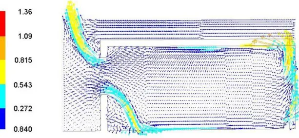
Results in the plane of the pole P2-P3-P5 is shown on Figure 11. It clearly indicates that the baseboard heater generates the convection. The air is escaping from the experimental chamber and directly goes to the ceiling of the facility where it gets cooler and goes down. Cool air enters the experimental chamber in the bottom of the window. This fresh air directly goes to the floor and goes near the baseboard.

Figure 11: Air Velocity Vectors in the plan P1-P5.

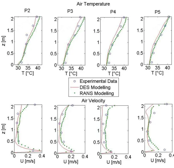
Figure 12 shows the comparison of the numerical and the experimental results. It clearly proves that once again CFD software is able to predict correctly air temperature. Gradients are also quite well captured.

Concerning air velocities, as before, results are not as good but mean value is good. It is impossible to know if the difference comes from difficulty to measure experimentally very low air velocities or if it is a CFD failing.

(13)

13

Figure 12: Results for the Natural Ventilation Case.

DES modelling is giving really interesting results. It permits to gain a lot of time compared to LES and results looks closer than with a RANS technique. The objectives of DES are achieved.

It is also interesting to check the value obtained for the air exchange rate. Indeed, this value is very important for air quality prediction. Experimentation gives a rate varying inside the range 6.75-7.92. Results with CFD software are 7.95 with RANS simulations, 7.7 with DES and 6.97 with LES (Jiang and Chen, 2003). So results are very good, especially for DES and LES. Note also that CFD is needed to have a good idea of this variable. Indeed, a previous study (Barbason et al., 2010) proved that multizone simulation overestimates the air exchange rate.

The paper of Jiang and Chen (2003) is also interesting because it focuses on a secondary variable (turbulent kinetic energy spectra). This is not done in this paper but the conclusion of Jiang and Chen is that LES (and probably DES) is the only way to have access to accurate results for secondary variables.

(14)

14

CFD is able to predict with accuracy natural ventilation. Every primary variable, ACH rate included, is correctly predicted. Once again, the operator can choose between RANS and LES techniques. Reliability in the results is guaranteed. Nevertheless, LES results gives better results providing to have required computing time and resources.

Concerning secondary variables, Jiang and Chen proved that the only way to model them correctly is to use a LES approach.

It should be noted that to converge to the good results with DES, DES model constants have evolved because results were not good in the first approach. So, even if DES gives better results, it is also because experimental results were known. For a preliminary design of a new building such results are not available. So the operator needs experience in DES modelling and there is still a risk to have wrong results.

6. CONCLUSION

Every operator should be aware of the impact of its choice and especially to understand the stakes of turbulence modelling. It is also important to make the choice in function of computing time and resources available.

LES, DES and RANS simulations give access to accurate results for primary variables which permit to predict occupant’s thermal comfort and air quality. As architects and building designers are generally interested only in these aspects, RANS technique is sufficient. Indeed, computing time and resources speak in favour of RANS simulations. However, results of LES simulations are better and give access to complementary data (secondary variables – turbulent aspects for example). These pieces of information are sometimes very interesting and necessary.

Eventually, the operator should know that numerical results can be wrong if LES parameters are not correctly chosen. Nevertheless, LES is able to model correctly every common situation in building physics. Without the slightest doubt, CFD will be more and more used and will provide always better results to help architects and building designers in their understanding of physical phenomena occurring in building physics.

ACKNOWLEDGEMENT

This research is a part of the SIMBA project. It is supported by the European Regional Development Fund (ERDF) and the Walloon Region.

REFERENCES

Barbason M., and Reiter S., 2010. About the choice of a turbulence model in building physics simulations. Proceedings of the 7th Conference on Indoor Air Quality, Ventilation and Energy Conservation in buildings (IAQVEC 2010), 1-8.

Barbason M., van Moeseke G., and Reiter S., 2010. A validation process for CFD use in building physics. Proceedings of the 7th Conference on Indoor Air Quality, Ventilation and Energy Conservation in buildings (IAQVEC 2010), 1-8.

Chen Q., and Srebric J., 2001. How to verify, validate, and report indoor environment modeling CFD analysis. ASHRAE RP-1133.

(15)

15

Cook M.J., and Lomas K.J., 1997. Guidance on the use of computational fluid dynamics for modelling buoyancy driven flows. Proceedings of the IBPSA Building Simulation ’97, 3, 57-72.

Hu J., Zuo W., and Chen Q., 2010. Impact of time-splitting schemes on the accuracy of FFD simulations. Proceedings of the 7th Conference on Indoor Air Quality, Ventilation and Energy Conservation in buildings (IAQVEC 2010), 1-8.

Jiang, Y., and Chen, Q., 2003. Buoyancy-driven single-sided natural ventilation in buildings with large openings. International Journal of Heat and Mass Transfer, 46, 973-988.

Jiang Y., Alloca C., and Chen Q., 2004. Validation of CFD simulations for natural ventilation. International Journal of Ventilation, 2(4), 359-370.

Kuznik F., Rusaouën G., and Brau J., 2007. Experimental and numerical study of a full scale ventilated enclosure: Comparison of four two equations closure turbulence models. Building and Environment, 42, 1043-1053.

Lampitella, P., 2009. The quality and reliability of large eddy simulation in a commercial CFD software. PhD Thesis, Second University of Naples, Naples, Italy.

Méndez C., San José J. F., Villafruela J. M., and Castro F., 2008. Optimization of a hospital room by means of CFD for more efficient ventilation. Energy and Buildings, 40, 849-854.

Menter F.R., 1994. Two-equation eddy-viscosity turbulence models for engineering applications. AIAA Journal, 32(8), 1598-1605.

Nicoud F., and Ducros F., 1999. Subgrid-Scale Stress Modelling Based on the Square of the Velocity Gradient Tensor. Flow, Turbulence, and Combustion, 62(3), 183-200.

Papakonstantinou K. A., Kiranoudis C. T., and Markatos N. C., 2000. Computational analysis of thermal comfort: the case of the archaeological museum of Athens. Applied Mathematical Modelling, 24, 477-494.

Tang D., and Robberechts B., 1989. Interzone convective heat transfer and air flow patterns. Report of Laboratory of Thermodynamics, University of Liege (Belgium).

Tang D., 1998. CFD modelling and experimental validation of air flow between spaces. Proceedings of the 6th International Conference on Air Distribution in Rooms – Roomvent 98, 2, 547-554.

Voigt L. K., 2000. Comparison of turbulence models for numerical calculation of airflow in an annex 20 room. Technical report, Danish Technical University of Lyngby.

Wang M., and Chen Q., 2010, Test of various turbulence models for airflow in enclosed environments. Proceedings of the 7th Conference on Indoor Air Quality, Ventilation and Energy Conservation in buildings (IAQVEC 2010), 1-8.

Yang C., Yang X., Xu Y., and Srebric J., 2007. Contaminant Disperson in personal displacement ventilation. Proceedings of the IBPSA Building Simulation 2007, 818-824.