HAL Id: hal-00841480
https://hal.archives-ouvertes.fr/hal-00841480
Submitted on 7 Jul 2013
HAL is a multi-disciplinary open access
archive for the deposit and dissemination of
sci-entific research documents, whether they are
pub-lished or not. The documents may come from
teaching and research institutions in France or
abroad, or from public or private research centers.
L’archive ouverte pluridisciplinaire HAL, est
destinée au dépôt et à la diffusion de documents
scientifiques de niveau recherche, publiés ou non,
émanant des établissements d’enseignement et de
recherche français ou étrangers, des laboratoires
publics ou privés.
Vector Lifting Schemes for Stereo Image Coding
Mounir Kaaniche, Amel Benazza-Benyahia, Béatrice Pesquet-Popescu,
Jean-Christophe Pesquet
To cite this version:
Mounir Kaaniche, Amel Benazza-Benyahia, Béatrice Pesquet-Popescu, Jean-Christophe Pesquet.
Vec-tor Lifting Schemes for Stereo Image Coding. IEEE Transactions on Image Processing, Institute of
Electrical and Electronics Engineers, 2009, 18 (11), pp.2463-2475. �hal-00841480�
Vector Lifting Schemes for Stereo Image Coding
M. Kaaniche, Student Member IEEE, A. Benazza-Benyahia, Member IEEE, B. Pesquet-Popescu, Senior
Member IEEE,
and J.- C. Pesquet, Senior Member IEEE
Abstract— Many research efforts have been devoted to the improvement of stereo image coding techniques for storage or transmission. In this paper, we are mainly interested in lossy-to-lossless coding schemes for stereo images allowing progressive reconstruction. The most commonly used approaches for stereo compression are based on disparity compensation techniques. The basic principle involved in this technique first consists of estimating the disparity map. Then, one image is considered as a reference and the other is predicted in order to generate a residual image. In this work, we propose a novel approach, based on Vector Lifting Schemes (VLS), which offers the advantage of generating two compact multiresolution representations of the left and the right views. We present two versions of this new scheme. A theoretical analysis of the performance of the considered VLS is also con-ducted. Experimental results indicate a significant improvement using the proposed structures compared with conventional methods.
I. INTRODUCTION
The principle of stereoscopic imaging systems consists of generating two images by recording two slightly different view angles of the same scene. By presenting the appropriate image of a stereo pair to the left/right eye, the viewer perceives the scene in three dimensions (3D). The recent advances in acqui-sition and display technologies have allowed the widespread use of stereovision in various application fields such as en-tertainment, medical surgical environments, tele-presence in videoconferences [1], computer vision and remote sensing [2]. For instance, today’s advances in satellite remote sensing technology provide the capability to collect Stereo Image (SI) pairs for several applications, such as cartography and urban planning. Satellite stereo images (such as those generated by IKONOS and SPOT5 sensors) are especially helpful to generate a digital elevation model which is a 3D representation of the topography of a given area [3]. The increasing interest in SIs has led to the constitution of image databases that require huge amounts of storage capacity. For example, the SPOT5 sensor covers areas of 60 Km × 60 Km at a resolution of 2.5 m and a single view requires more than 500 Megabytes. In addition to these stereo sensors, it is worth mentioning the Multi-angle Imaging SpectroRadiometer (MISR), which uses nine cameras to generate multiview data sets [4] at a data rate of 3.3 Mbps. Hence, the use of compression techniques is mandatory for image storage as well as for image transmission.
M. Kaaniche and B. Pesquet-Popescu are with the Ecole Nationale Sup´erieure des T´el´ecommunications de Paris, 37-39 rue Dareau 75014 Paris, France. E-mail: [email protected], [email protected]. A. Benazza-Benyahia is with the Ecole Sup´erieure des Com-munications de Tunis (SUP’COM-Tunis), 2083, Tunisia. E-mail: [email protected]. J.-C. Pesquet is with the Universit´e Paris-Est, Laboratoire d’Informatique Gaspard Monge, CNRS UMR 8049, 77454 Marne-la-Vall´ee, France. E-mail: [email protected].
Part of this work has been presented in [21].
To the best of our knowledge, the ongoing activity on stereo-scopic still image coding is mainly carried out independently of any standardization activity [5]. Consequently, different approaches have been reported concerning still image coding. The most simple ones consists of separately coding each view by using existing still image coders. However, the resulting data rates may remain too high for some practical stereoscopic systems. As the two images have similar content, they are highly correlated. Therefore, more efficient coding schemes have been designed to exploit the cross-view redundancies [6], [7]. This is usually achieved by first estimating the disparity field between the SI pair [8]. Then, one image is considered as a reference (say the left one) and the other image (target) is predicted by disparity-compensating the reference one. A prediction error image, called residual image, is thus generated. Finally, the disparity field, the reference image and the residual one are encoded [7], [9]. This approach is known as disparity compensation due to its similarity with motion compensation techniques which are popular for video coding [10]. The goal of this paper is to design a novel joint coding approach enabling a gradual and finally exact decoding of the stereo pairs. Our main contribution is that the proposed coding scheme does not generate any residual image, but directly two compact multiresolution representations of the left and right images by exploiting the cross-view redundancies via the available disparity field. Furthermore, the proposed scheme is intrinsically flexible, as it allows the designer to optimize the number of prediction filter taps as well as the other parameters of the multiscale operators. In this way, we build a joint coding scheme which is adapted to the content of the stereo pair. Another advantage of the proposed method is that it guarantees a perfect reconstruction of the stereo images.
The remainder of this paper is organized as follows. Sec-tionIIgives an overview of SI coding schemes based on dis-parity estimation and compensation techniques. In SectionIII, we propose a novel coding structure of which two examples are given. In Section IV, we conduct a theoretical analysis of the proposed schemes in terms of prediction efficiency. Section V describes how embedded binary streams can be produced to encode the resulting multiscale representations. Finally, in SectionVI, experimental results are given and some conclusions are drawn in Section VII.
II. STEREOIMAGECODING
Generally, the reported stereo image coding methods rely on Disparity Estimation techniques (DE) followed by Disparity Compensation (DC) as discussed below. As mentioned earlier, DE is a key issue for exploiting the cross-view redundancies. This problem has been extensively studied in computer vision
and surveys of the different DE techniques proposed in the literature can be found in [2], [11], [12]. Two main approaches, pixel-based or block-based, can be used to estimate the dispar-ity map. In what follows, we use a fixed size block matching DE, which consists of first partitioning the right image I(r) into nonoverlapping blocks of size bx× by. For each block, the objective is to find the most “similar” block within a given search area S in the left image I(l). The disparity vector v = (vx, vy) for a current block in I(r) minimizes a dissimilarity criterion D: (vx, vy)(mx, my) △ = arg min (vx,vy)∈S D(I(r)(m x, my), I(l)(mx+ vx, my+ vy)) (1) where (mx, my) are the spatial coordinates associated with the top leftmost pixel in the block. Very often, the Sum of Square Differences (SSD) or the Sum of Absolute Differences (SAD) is the selected criterion. It should be noted that in the ideal parallel-axis geometry, the displacement between the two views is restricted to the horizontal direction (vy = 0) and it takes positive values (vx ≥ 0). However, in practice, the matching point of any current point of I(r) is not always rigorously on the epipolar line because of the sensor noise, the discretization errors and the deviation from the pinhole camera model. As a consequence, a strip along the epipolar line is considered and all the points falling within this strip are considered as potential matching candidates to be paired with the current point. It is worth mentioning that several works aimed at improving this block-based DE, e.g. by using overlapped block DE with adaptive windows [13], [14]. Once the disparity vectors are generated, a disparity compensation can be performed: the target imageI(r) is predicted fromI(l) along the disparity vectors. Then, the Disparity Compensated Difference (DCD) I(e) is computed as follows:
I(e)(mx, my) △
= I(r)(mx, my) − I(l)(mx+ vx, my+ vy) (2) where the dependence on (mx, my) of vx and vy has been dropped for notation simplicity. Generally, the disparity vec-tors are losslessly encoded using DPCM followed by arith-metic encoding, whereas the reference and the residual images can be coded in different transform domains. Some works ap-ply a discrete cosine transform [9], [15]. However, more recent works have preferred the wavelet transform, in order to meet the scalability requirement. In [16], an efficient exploitation of the zerotree algorithm [17] is performed to shorten the embedded bitstreams of the wavelet coefficients of both the reference image and the DCD. In [18], both the estimation and the disparity compensation take place in the wavelet domain, the coding of the wavelet coefficients being performed through a Subspace Projection Technique (SPT). Furthermore, we should note also that Annex I of Part II of the JPEG2000 standard is dedicated to multi-component image coding [19]. A decorrelation of the spectral components may be performed prior to the wavelet transform. In our case, each view of the stereoscopic image can be seen as a single component. Unlike
the conventional methods, we propose a joint coding scheme that directly generates a pair of multiresolution representations of the left and the right images derived from a judicious lifting decomposition which will be described in the next section.
III. PROPOSED VECTOR LIFTING SCHEMES
A. Motivations
A novel approach that is based on a joint multiscale decomposition of I(l) and I(r) is developed in this section. It consists of coding the reference image I(l) in intra mode (purely spatial), whereas the other image is coded by exploit-ing cross-image redundancies via the available disparity map. The decomposition strategy is inspired from Vector Lifting Schemes (VLS) [20] and it has been briefly presented as a preliminary work in [21]. The main advantage of the proposed approach is that it does not explicitly generate a residual image, but two multiresolution representations ofI(l)andI(r). Two versions of the VLS will be described in the following.
B. VLS decompositions
The wavelet coefficients of an image are usually obtained by a dyadic filter bank structure [22]. If an exact recon-struction is required, lifting schemes are often employed, since they allow to generate integer-valued versions of the wavelet coefficients whatever the underlying decomposition operators are [23], [24]. For the sake of simplicity, a separable decomposition is considered in this paper. Therefore, it is enough to address the decomposition in one dimension. The corresponding analysis structure is shown in Fig. 2. More precisely, at each resolution levelj, the even and odd samples of the approximation (scaling) coefficients Ij(l)(mx, 2my), Ij(r)(mx, 2my), Ij(l)(mx, 2my + 1) and Ij(r)(mx, 2my + 1) of I(l) andI(r) respectively are the input coefficients of the lifting scheme. Furthermore, we denote by vj = (vx,j, vy,j)⊤ the available disparity vectors which are obtained by sampling and dividing by2j
the initial (full resolution) disparity vectors v= (vx, vy)⊤, since the dimensions of the subbands at the j-th resolution level correspond to j-the dimensions of j-the initial images divided by2j: vj(mx, my) = 1 2jv(2 jm x, 2jmy). (3)
It is important to note that (3) may yield non-integer values of the disparity vectors. Therefore, if the components of vj are integer-valued, for any given pixel(mx, my) in the right image corresponds a pixel in the disparity-compensated left image Ij(l)(mx+ vx,j(mx, my), my+ vy,j(mx, my)). Otherwise, the corresponding disparity-compensated intensity results from the usual bilinear interpolation. The objective of the vector lifting scheme is to simultaneously exploit the dependence existing betweenIj(l)andI
(r)
j by producing 2 kinds of outputs: the de-tail coefficients ed(l)j+1, ed(r)j+1 and the approximation ones eIj+1(l) , e
Ij+1(r) for both images. Similar lifting structures operating along the image columns allow us to generate the approximation coefficients Ij+1(l) and I
(r)
j+1, as well as the associated detail coefficients in the horizontal, vertical and diagonal directions
at the resolution level (j + 1).1 A wide range of nonlinear operators can be applied to reduce the intra and inter-image redundancies. However, for tractability purposes, we will only use combinations of shift operators, linear filters and rounding operations. For the reference imageI(l), the detail coefficients can be interpreted as intra-image prediction errors at resolution (j + 1) and expressed as:
e d(l)j+1(mx, my) = I (l) j (mx, 2my+ 1) − ⌊(P (l) j )⊤I (l) j ⌋ (4) where P(l)j = ³ p(l)j,k ´
k∈Pj(l) is the prediction weighting vector, I(l)j = ³Ij(l)(mx, 2my− 2k)
´
k∈Pj(l) is the reference vector containing the even samples used in the prediction step,Pj(l) is the support of the predictor of Ij(l)(mx, 2my + 1) and ⌊.⌋ is the integer-part operator. Then, at the update step, the approximation coefficients are computed as follows:
e Ij+1(l) (mx, my) = Ij(l)(mx, 2my) + ⌊(U(l)j ) ⊤ed(l) j+1⌋ (5) where U(l)j = ³ u(l)j,k´
k∈Uj(l) is the update weighting vector, e
d(l)j+1 = ³de(l)j+1(mx, my− k) ´
k∈Uj(l) is the reference vector containing the details coefficients used in the update step, and Uj(l) is the support of the update operator. The reversibility of the basic lifting scheme is ensured since the prediction in (4) only makes use of even indexed samples. The main difference between a vector lifting scheme and a basic one is that for the image I(r), the prediction of the odd sample Ij(r)(mx, 2my + 1) involves even samples from the same image and also neighbors of the matching sample taken from the reference image. For the sake of simplicity, the notation Ij(l)(mx+ vx,j(mx, my), my + vy,j(mx, my) − k) which corresponds to the compensated image on the neighbors of a given matching sample (mx, my), will be replaced by Ij(c)(mx, my, k). Thus, the detail signal ed(r)j+1will be expressed as: e d(r)j+1(mx, my) = I (r) j (mx, 2my+ 1) − ⌊(P (r) j ) ⊤I(r) j + (P(r,l)j ) ⊤I(c) j ⌋ (6) where P(r)j =³p(r)j,k ´ k∈Pj(r) (resp. P (r,l) j = ³ p(r,l)j,k ´ k∈Pj(r,l)) is the prediction weighting vector of the intra-image (resp. inter-images), I(r)j =³Ij(r)(mx, 2my− 2k)
´
k∈Pj(r) is the reference vector containing the even samples, I(c)j =
³
Ij(c)(mx, 2my+ 1, k)´
k∈Pj(r,l) is the vector containing the neighbors of the matching sample associated with the pixelIj(r)(mx, 2my+ 1) to be predicted, andPj(r)(resp.P
(r,l)
j ) is the spatial support of the intra-image (resp. inter-images) predictor. The update step for eIj+1(r) can be performed similarly to (5). The decomposition is iterated on the columns my of the resulting subbands,
1As we apply a separable decomposition, we denote by eI
jthe
approxima-tion coefficients after the first mono-dimensional processing at the jthlevel, and by Ijthe final approximation subband.
leading to 2 × 4 sub-images for the left and right images at each resolution level j and the decomposition is again repeated on the approximation sub-images over J resolution levels. It is worth pointing out that the disparity based vector lifting scheme is perfectly reversible and that it maps integers to integers. However, an appropriate choice of the involved prediction and update operators remains necessary in order to generate compact representations of (I(l), I(r)). To illustrate the ability of the considered vector lifting structure to produce a sparse representation, we provide a simple example (denoted by VLS-I) of the considered lifting structure. The image I(l) is first decomposed following the well-known integer-to-integer 5/3 scheme employed for the lossless mode of JPEG 2000 [23]. According to our notations, the spatial supports for the prediction and update operators are: Pj(l) = {−1, 0}, Uj(l)= {0, 1} and their related weights are: p
(l)
j,−1= p
(l) j,0= 12, u(l)j,0= u(l)j,1= 1
4. The hybrid intra-inter prediction step related to I(r) is then expressed via the following spatial supports: Pj(r)= {−1, 0}, P
(r,l)
j = {0}. In other words, the prediction mask contains the same spatial prediction indices as those used in the5/3 scheme and the co-located position in the left image. As the detail coefficients can be viewed as prediction errors, the prediction coefficients p(r)j,k and p
(r,l)
j,k can be optimized at each resolution level by solving the well-known Yule-Walker equations. Concerning the update step, it is possible to generalize the optimization procedure described in [25], [26] in order to adapt the underlying operators to the statistical properties of the input image. A straightforward alternative solution that we preferred in our experiments consisted of choosing the same update operator at all resolution levels, the update employed forI(r) being the same as the two-tap filter employed for I(l) in Eq (5).
C. An improved VLS
One of the potential drawbacks of the previous VLS-I structure is that it generates an update leakage effect, in the sense that the information coming from the left view, which is used for the prediction of the right one, is also used, through the update operator, to compute the approximation coefficients of the right view. An alternative solution is given by the predict-update-predict (P-U-P) lifting structure shown in Fig.3. The improved decomposition is described as follows:
e d(r)j+1(mx, my) = Ij(r)(mx, 2my+ 1) − ⌊(P(r)j ) ⊤I(r) j ⌋, (7) e Ij+1(r)(mx, my) = Ij(r)(mx, 2my) + ⌊(U(r)j ) ⊤de(r) j+1⌋, (8) ˇ d(r)j+1(mx, my) = ed (r) j+1(mx, my) − ⌊q⊤jeI (r) j+1 + (P(r,l)j ) ⊤I(c) j ⌋, (9) where notations similar to those used in Section III-B are used and qj = (qj,k)k∈Qj is the second intra-image predictor associated to the reference vector eI(r)j+1 = ³
e
Ij+1(r)(mx, my− k) ´
k∈Qj
. It is worth noting that a prediction and an update as in (7) and (8) (with the same weights) are applied to I(l). In addition, at the last resolution level
j = J, instead of directly coding the approximation IJ(r), we predict it from the approximation subband at the last level of the disparity-compensated image and only code the residual subbande(r)J given by:
e(r)J (mx, my) = IJ(r)(mx, my) − ⌊(P(r,l)J ) ⊤I(c) J ⌋ (10) where P(r,l)J =³p(r,l)J,k ´ k∈PJ(r,l) and I (c) J = ³ IJ(c)(mx, my, k) ´ k∈PJ(r,l). Let the coefficients qj,k and p(r,l)j,k (resp.p
(r,l)
J,k ) be optimized so as to minimize the variance of ˇd(r)j+1 (resp. e(r)J ) at each resolution levelj < J (resp. at the coarsest resolution level J). An interesting property of the proposed decomposition is the following: in the ideal situation corresponding toI(l) = I(r), the multiresolution representation ofI(r)reduces to zero under some constraints that we are going to define in the following. Indeed, in the ideal case whenI(l)= I(r), the disparity vectors are zero: (vx, vy) = (0, 0). Therefore, (9) becomes:
ˇ d(r)j+1(mx, my) = ed (r) j+1(mx, my) − ⌊q⊤jeI (r) j+1+ (P (r,l) j ) ⊤I(l) j ⌋ = Ij(r)(mx, 2my+ 1) − ⌊ X k∈Pj(r) p(r)j,kIj(r)(mx, 2my− 2k)⌋ − ⌊X k∈Qj qj,kIe (r) j+1(mx, my− k) + X k∈Pj(r,l) p(r,l)j,k Ij(l)(mx, 2my+ 1 − k)⌋. (11)
It is worth pointing out that the coefficients qj,k and p(r,l)j,k are optimized, at each decomposition level, by solving the Yule-Walker equations, the rounding operator being omitted. Thus, the detail coefficients ˇd(r)j+1(mx, my) can be viewed as the errors involved in the prediction of ed(r)j+1(mx, my) by the signal t(mx, my) = Pk∈Qjqj,kIej+1(r) (mx, my − k) +Pk∈P(r,l)
j
p(r,l)j,k Ij(l)(mx, 2my+ 1 − k). In this way, we can ensure that the detail coefficients of the right image
ˇ
d(r)j+1(mx, my) are zero if the prediction signal t(mx, my) is a linear combination of (at least) the same samples as those used by the reference signal ed(r)j+1(mx, my) to be predicted. This can be guaranteed provided that the support of the hybrid predictor Pj(r,l) satisfies the two following conditions:
(i) The first termIj(r)(mx, 2my+ 1) in the expression of ed(r)j+1(mx, my) in Eq. (7) can be found in the expression of the prediction signal t(mx, my) if 0 ∈ Pj(r,l).
(ii) The second term in the expression of ed(r)j+1(mx, my) involves the samples (Ij(r)(mx, 2my − 2k))k∈P(r)
j . These samples can be found in the expression of the prediction signalt(mx, my) if {2k + 1, k ∈ P
(r)
j } ⊂
Pj(r,l).
When the conditions (i) and (ii) are satisfied andIj(l)= I (r)
j ,
the decomposition of Ij(r) first provides a detail subband ˇ
d(r)j+1(mx, my) which is equal to zero and an approximation subband eIj+1(r) which is equal to that ofI
(l) j : eI
(r)
j+1(mx, my) = e
Ij+1(l) (mx, my). Then, while processing the image along the columns, the decomposition of eIj+1(r) generates in the same way a detail subband which is equal to zero and an approximation subbandIj+1(r) which is equal to that of eIj+1(l) :Ij+1(r) (mx, my) = Ij+1(l) (mx, my). Finally, the decomposition of ˇd(r)j+1 provides two null detail subbands since ˇd(r)j+1(mx, my) = 0. Conse-quently, the resulting multiresolution representation of Ij(r) based on the new scheme allows us to generate an approx-imation subband which is identical to that of Ij(l) and three detail subbands equal to zero. Since at each resolution level the approximation subbands ofIj(r)andI
(l)
j are equal, the residual sub-image e(r)J in (10) becomes null if0 ∈ P
(r,l)
J . Therefore, the P-U-P decomposition satisfies the property of cancelling the values of the wavelet coefficients of the multiresolution representation ofI(r)provided that{0}∪{2k+1, k ∈ P(r)
j } ⊂
Pj(r,l), whenj < J, and 0 ∈ P (r,l)
J . This is a desirable property of the considered decomposition in order to get a consistent joint representation ofI(l) andI(r). In contrast, this property does not hold for VLS-I.
Finally, as a supporting example, we design a scheme, which will be denoted in the following by VLS-II, by adding a prediction stage to the conventional 5/3 lifting structure. This amounts to choose Pj(r) = {−1, 0}, U (r) j = {0, 1}, and p(r)j,−1 = p (r) j,0 = 12, u (r) j,0 = u (r)
j,1 = 14, while the last prediction stage is performed by setting Qj = {−1, 0}, and Pj(r,l)= {−3, . . . , 3} for j ∈ {0, . . . , J −1} and P
(r,l) J = {0}. The coefficientsqj,k andp
(r,l)
j,k are determined by solving the Yule-Walker equations (still omitting the rounding operations) and imposing again the symmetry properties:qj,−1= qj,0and p(r,l)j,k = p(r,l)j,−k (which allows us to obtain linear phase filters often considered as desirable for image coding [27]).
IV. THEORETICAL ANALYSIS
In this section, we perform a theoretical analysis of the performances of VLS-I and VLS-II in terms of prediction efficiency, which is directly related to the coding efficiency [28], [29]. Firstly, we give the explicit expressions of the optimal prediction coefficients as well as the variance of detail signals for the two schemes. Then, we confirm that the prediction error variance of VLS-II is smaller than the one of VLS-I.
A. Notations
In the following, we will develop our analysis in the case of 1D signals, since we have considered a separable scheme. More precisely, let (mx, my) be a given pixel, we consider
the pair of 1D signals defined for alln ∈ Z by: i(r)j (n) = I (r) j (mx, n) i(l)j (n) = Ij(l)(mx+ vx,j(mx, 2my+ 1), n + vy,j(mx, 2my+ 1)). (12) We assume that, at a given resolution level j, these signals satisfy the following symmetric linear statistical model:
(
i(r)j (n) = αjaj(n) + βjbj(n) i(l)j (n) = βjaj(n) + αjbj(n)
(13) where (αj, βj) ∈ R2 such that α2j + β2j = 1, and aj and bj are two stationary random processes which are mutually independent. For the sake of simplicity, we assume that they are zero-mean (which is always verified for wavelets coefficients) and they have the same autocorrelation function Rj withRj(0) > 0. Then, it is easy to show that:
Ehi(r)j (n)i (r) j (n − k) i = Ehi(l)j (n)i (l) j (n − k) i = Rj(k), (14) Ehi(r)j (n)i (l) j (n − k) i = sjRj(k) (15) where sj △ = sin(2θj) and θj △ = arg(αj+ ıβj) (with ı2 = −1). At this point, it is worth noticing that the spatial similari-ties between the samples of i(r)j (or i
(l)
j ) are related to the autocorrelation function Rj. The factorθj controls the cross-redundancies between the samples of i(r)j andi(l)j .
B. Minimum prediction error variance of VLS-I
By considering the support and the weights of the predic-tion operator involved in VLS-I (still omitting the rounding operators), the detail signal ed(r)j+1(n) is expressed as follows:
e d(r)j+1(n) =i (r) j (2n + 1) − p (r) j,0 ³ i(r)j (2n) + i (r) j (2n + 2) ´ − p(r,l)j,0 i (l) j (2n + 1). (16) Thus, ed(r)j+1(n) can be viewed as the error in the predic-tion of i(r)j (2n + 1) by the multivariate reference signal ij(n) △ =³i(r)j (2n) + i (r) j (2n + 2), i (l) j (2n + 1) ´⊤ . The predic-tion weight vector pj = (p
(r) j,0, p
(r,l)
j,0 )⊤ satisfies the normal equations: E£ij(n)ij(n)⊤ ¤ pj= E h i(r)j (2n + 1)ij(n) i . (17) Hence, the optimal weights can be deduced as follows:
( p(r)j,0 = γ1,j(θj)Rj(0)Rj(1)(s2j− 1) p(r,l)j,0 = γ1,j(θj)sj ³ 2Rj(1)2− Rj(0)2− Rj(0)Rj(2) ´ (18) where γ1,j(θj) △ =¡2s2 jRj(1)2− Rj(0)2− Rj(0)Rj(2) ¢−1 . Consequently, the minimum value ε1,j of the prediction error
variance achieved by VLS-I is: ε1,j(Rj, θj) =E h i(r)j (2n + 1) 2i− p⊤ jE h i(r)j (2n + 1)ij(n) i =γ1,j(θj) cos2(2θj)Rj(0) ³ 2Rj(1)2− Rj(0)2 − Rj(0)Rj(2) ´ . (19)
C. Minimum prediction error variance of VLS-II
Considering now VLS-II (still omitting the rounding oper-ators), the detail signal ˇd(r)j+1(n) is given by:
ˇ d(r)j+1(n) = i (r) j (2n + 1) − 1 2 ³ i(r)j (2n) + i (r) j (2n + 2) ´ − qj,0 ³ ei(r) j+1(n) + ei (r) j+1(n + 1) ´ − p(r,l)j,0 i (l) j (2n + 1) − 3 X k=1 p(r,l)j,k ³ i(l)j (2n + 1 − k) + i (l) j (2n + 1 + k) ´ (20) where, as shown by (8), the signal ei(r)j+1(n) can be expressed as: ei(r) j+1(n) = i (r) j (2n) + 1 4 ³ e d(r)j+1(n − 1) + ed(r)j+1(n)´ = 1 4 ³ 3i(r)j (2n) + i(r)j (2n + 1) + i(r)j (2n − 1)´ −1 8 ³ i(r)j (2n − 2) + i (r) j (2n + 2) ´ . (21)
Therefore, it can be checked that: ˇ dj+1(n) = rj(n) − qj,0uj(n) − p (r,l) j,0 i (l) j (2n + 1) − 3 X k=1 p(r,l)j,k ³ i(l)j (2n + 1 − k) + i (l) j (2n + 1 + k) ´ (22) where rj(n) △ =i(r)j (2n + 1) − 1 2 ³ i(r)j (2n) + i (r) j (2n + 2) ´ , (23) uj(n) △ =1 2i (r) j (2n + 1) + 5 8 ³ i(r)j (2n) + i (r) j (2n + 2) ´ +1 4 ³ i(r)j (2n − 1) + i (r) j (2n + 3) ´ −1 8 ³ i(r)j (2n − 2) + i (r) j (2n + 4) ´ . (24)
From (22), ˇd(r)j+1(n) can be viewed as the error in the prediction of rj(n) by the reference samples grouped into the vector ˜rj(n) given by: ˜rj(n) △ =³uj(n), i(l)j (2n + 1), i (l) j (2n) + i (l) j (2n + 2), i(l)j (2n − 1) + i (l) j (2n + 3), i (l) j (2n − 2) + i (l) j (2n + 4) ´⊤ . (25) The vector pj = (qj,0, p(r,l)j,0 , p (r,l) j,1 , p (r,l) j,2 , p (r,l) j,3 )⊤ is found by minimizing the variance of ˇd(r)j+1(n). Consequently, the following set of normal equations Γjpj= cj must be solved where Γj = E
£
˜rj(n)˜rj(n)⊤ ¤
and cj = E [rj(n)˜rj(n)]. Once the auto-correlation matrix Γjand the cross-correlation vector
cjare determined, the optimal weights are obtained as follows: qj,0= − 4γ2,j ³ Rj(0) − 4Rj(1) + 4Rj(3) − Rj(4) ´ , (26) p(r,l)j,0 =γ2,jsj ³ 40Rj(0) + 48Rj(1) + 31Rj(2) + 20Rj(3) − 8Rj(4) − 4Rj(5) + Rj(6) ´ , (27) p(r,l)j,1 = − γ2,jsj ³ 33Rj(0) + 76Rj(1) + 31Rj(2) − 8Rj(3) − Rj(4) − 4Rj(5) + Rj(6) ´ /2, (28) p(r,l)j,2 =γ2,jsj ³ Rj(0) − 4Rj(1) + 4Rj(3) − Rj(4) ´ , (29) p(r,l)j,3 = − γ2,jsj ³ Rj(0) − 4Rj(1) + 4Rj(3) − Rj(4) ´ /2, (30) where γ2,j = ³ 38Rj(0) + 56Rj(1) + 31Rj(2) + 12Rj(3) − 6Rj(4) − 4Rj(5) + Rj(6) ´−1
. Finally, the minimal value of the variance ε2,j of the prediction error generated by VLS-II is: ε2,j(Rj, θj) = E £ rj2(n) ¤ − p⊤jE [rj(n)˜rj(n)] = 1 2γ2,jcos 2(2θ j) ³ 113Rj(0)2− 240Rj(1)2+ 31Rj(2)2 − 16Rj(3)2− Rj(4)2− 4Rj(1)Rj(6) + 28Rj(0)Rj(3) − 16Rj(0)Rj(4) + 131Rj(0)Rj(2) − 4Rj(2)Rj(5) + 3Rj(0)Rj(6) − 16Rj(1)Rj(3) + 16Rj(1)Rj(4) − 68Rj(1)Rj(2) + 16Rj(1)Rj(5) + 12Rj(2)Rj(3) + Rj(2)Rj(6) + 8Rj(3)Rj(4) + 24Rj(0)Rj(1) − 6Rj(2)Rj(4) − 12Rj(0)Rj(5) ´ . (31) D. Discussion
It should be noticed that the expressions of ε1,j and ε2,j are not restricted to a particular form of the autocorrelation function Rj, and so they are valid for any second-order stationary process. Furthermore, it is interesting to note that, unlike ε1,j, ε2,j is separable in Rj and θj. In order to emphasize the advantages of VLS-I and VLS-II, we will consider a simple multivariate random process model driven by two autoregressive processes of order 1, aj(n) and bj(n) in (13). In this particular case, the autocorrelation function is given by:
∀k ∈ Z, Rj(k) = σj2ρ |k|
j (32)
where ρj ∈ [−1, 1] is the correlation factor. Therefore, the variances ε1,j andε2,j of the prediction errors reduce to:
ε1,j(Rj, θj) =σ2jγ˜1,j(θj) cos2(2θj)(ρ2j− 1), (33) ε2,j(Rj, θj) = 1 2σ 2 jγ˜2,jcos2(2θj)(1 − ρj)(3ρ4j− 16ρ 3 j + 4ρ2j+ 24ρj+ 113), (34) where˜γ1,j(θj) = (2s2jρ2j− ρj2− 1)−1 andγ˜2,j = (ρ5j− 5ρ4j− ρ3 j+ 13ρ2j+ 18ρj+ 38)−1.
Furthermore, we can check that the variance of the intra prediction error generated by the 5/3 transform as indicated
by (23) is given by: Ehrj(n)2
i =1
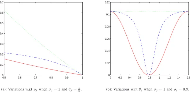
2(3 − ρj)(1 − ρj). (35) Fig. 4(a) shows the variations of Ehrj(n)2
i
, ε1,j and ε2,j with respect to ρj for a given value of θj. Thus, by taking into account the spatial redundancies (controlled by ρj), the variance ε1,j is smaller than E
h rj(n)2
i
. Lower values of the prediction error variance ε2,j are further achieved by the VLS-II transform for any value ofρj. We are also interested in comparing the variations of these three prediction errors with respect to θj for a given value of ρj, as depicted by Fig. 4(b). It can be noted that VLS-II gives also the best results by exploiting the inter-image redundancies (controlled by θj). This study has clearly shown the benefit that can be drawn from the use of VLS-II compared to VLS-I. This is explained by the proposed P-U-P structure in which the cross-view redundancies are exploited in the additional prediction step in order to avoid injecting the information coming from the reference image in the approximation of the target image.
V. EMBEDDED CODING OF STEREO IMAGES
A. Coding techniques
After applying a VLS to a stereo image pair, the generated coefficients must be encoded. However, the coding scheme should enable quality scalability for progressive reconstruction purposes. This is basically achieved by sending the coefficients in decreasing order of their importance. In other words, the most significant ones are first encoded at a reduced accuracy. So, a first approximation image is produced, which is further gradually refined by decoding the least significant coefficients. To this end, several scalable codecs have been developed [17], [30], [31], [32]. The main advantage of these embedded codecs is that the encoder can terminate the encoding at any point, thereby allowing a target bitrate to be exactly met. Similarly, the decoder can also stop decoding at any point resulting in the image that would have been produced at the rate corre-sponding to the truncated bitstream. In our experiments, we have employed the JPEG2000 codec, which yields excellent performance in terms of compression efficiency and quality scalability.
B. Transmission cost of the prediction coefficients
The prediction coefficients involved in the proposed VLS decompositions have to be transmitted to the decoder in order to proceed to the inverse transform with perfect reconstruction of the stereo pairs. The prediction weights correspond to an amount of op = 3 L J floating point coefficients, where L is the number of prediction weights in the VLS andJ represents the number of resolution levels (the factor 3 stems from the fact that one horizontal prediction and two vertical predictions, one in the low-pass horizontal subband and the other in the high-pass horizontal subband, are performed). These weights are stored on 32 bits, inducing a negligible increase of the overall bitrate. More precisely, for a stereo pair of sizeNx× Ny, the transmission cost of the prediction coefficients will
increase the bitrate achieved by VLS-I and VLS-II, by op
2NxNy bits per pixel. For example, whenNx= Ny= 512 and J = 2, the gain will be decreased by 0.0007 bpp (resp. 0.0018 bpp) in the case of VLS-I (resp. VLS-II) which is a very small fraction of the whole data bitrate.
VI. EXPERIMENTAL RESULTS
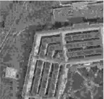
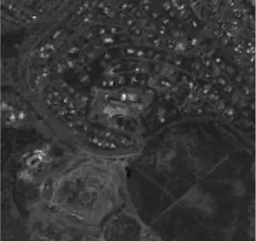
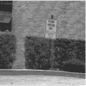
Simulations have been carried out on 6 image pairs of size 512 × 512 which have been extracted from a SPOT5 scene. The full scene, which corresponds to an urban zone, is shown in Fig. 1 and the six image pairs are represented in white squares. We have also used 4 pairs of natural stereo images (“fruit”, “pentagon”, “shrub” and “birch”) downloaded from 2 and 3. It should be noted that some stereo images have significant illumination variations between the views. For this reason, DC is performed by applying to the original SI the reversible remapping technique based on sorting permutations introduced in [33]. This preprocessing step is often used to improve the coding efficiency of pairs of images [34]. The disparity map is computed using a block-matching technique with a 8 × 8 block size and a search area that depends on the acquisition of the stereo pair (+50 pixels in the horizontal direction and ±2 in the vertical direction for SPOT5 stereo images, and +30 pixels in the horizontal direction and ±4 in the vertical direction for natural stereo images). The SSD is the chosen matching criterion. The resulting disparity vectors are losslessly encoded using a median prediction and DPCM with arithmetic encoding. In order to show the benefit of the joint coding by VLS, we compare VLS-I and VLS-II decompositions carried out over J = 2 resolution levels with some representative SI wavelet-based coding methods: • The first one is the baseline coder which consists of coding the left image I(l) and the DC-residual I(e) with a 5/3 transform [16]. In the following, this method will be designated by scheme B.
• The second one is the subspace projection technique in the wavelet domain (SPT-WT) proposed by Jiang et al. [18]. This method consists of applying the DE and DC steps in the wavelet domain. More precisely, the method starts by applying the 5/3 transform to the original SI pair. We denote by {a(r)J , (d(r,o)j )1≤j≤J, o ∈ {1, 2, 3}} (resp. {a(l)J , (d
(l,o)
j )1≤j≤J, o ∈ {1, 2, 3}}) the resulting
approxima-tion and detail subbands for the right (resp. left) image. A block-based DE is performed between the corresponding sub-bands(a(r)J , a (l) J ) and (d (r,o) J , d (r,o)
J ). Then, a DC of each block of the image subbands is carried out, leading to the predicted subbands{ˆa(r)J , ˆd
(r,o)
j , o ∈ {1, 2, 3}}. Finally, the computation of the DCD is obtained by projecting each block of the approx-imation subband of the target image a(r)j onto the subspace S = span{ˆa(r)J , ˆd
(r,o)
J , o ∈ {1, 2, 3}}, yielding the projection ˇ
a(r)J = α0ˆa(r)J + P3
o=1αodˆ(r,o)J where (α0, α1, α2, α3) are computed by a least squares approach. In our experiments, and in order to ensure a lossless reconstruction, we have encoded a
2http://vasc.ri.cmu.edu/idb/html/stereo/index.html 3http://vasc.ri.cmu.edu/idb/html/jisct/
rounded version ofˆa(r)j . Consequently, the approximation sub-band of the residual image is defined bya(e)J = a
(r) J − ⌊ˇa
(r) J ⌋, whereas the other detail subbands are simply computed as: d(e,o)j = d
(r,o)
j − ˆd
(r,o)
j o ∈ {1, 2, 3}.
• We have also tested a version of JPEG2000 (Annex I of Part II) dedicated to multicomponent images. It consists first of a decorrelation of the SI pair. Note that this decorrelation step must use a reversible transform in order to exactly recover the original SI pair. As a result, a pair ( ˜I, I(e)) is produced by using a variation of the Haar transform [35]:
I(e)(m x, my) = I(r)(mx, my) − I(l)(mx+ vx, my+ vy), ˜ I(mx+ vx, my+ vy) = ⌊(I(l)(mx+ vx, my+ vy) +I(r)(m x, my))/2⌋ if(mx+ vx, my+ vy) ∈ S, ˜ I(mx, my) = I(l)(mx, my) if (mx, my) 6∈ S. (36) whereS is the set of connected pixels in the left image. Then, the 5/3 transform is separately applied to I(e) and ˜I. This method will be designated in the following by scheme C. The compression measure is given by the final bitrates of the multiresolution representations. Let us denote by R(v),R(l), R(r) andR(e), respectively, the bitrate of the disparity vectors v and of the imagesI(l),I(r)andI(e). For the methods based on the coding of the residual image, we have computed the following average bitrate:
Rav = R
(l)+ R(e)+ R(v)
2 (37)
while the average bitrate for the proposed decompositions is given by:
Rav =R
(l)+ R(r)+ R(v)
2 . (38)
It can be noticed that the average coding cost R(v) of the losslessly encoded disparity vectors is around 0.07 bpp. Table I provides the final bitrates obtained in a lossless context by applying the JPEG2000 codec used only as an entropy codec on the produced subbands. Our simulations indicate that VLS-I results in an average gain of about 0.1 bpp over conventional methods. If we now compare the performance of VLS-II to those provided by VLS-I, our experiments show that VLS-II leads to a further improvement of about 0.1 bpp.
We have also tested the performance of our methods when applied as a lossy codec. In this case, the improved VLS are also compared in terms of Peak-Signal-to-Noise Ratio (PSNR) given by: PSNR = 10 log10 ³ 2552 (MSE(l)+ MSE(r))/2 ´ (39) where MSE(l) and MSE(r) respectively correspond to the mean squared error of the left and right images reconstructed at the rates R(l) and R(r). We also used the SSIM quality metrics, which is based on models of visual perceptions, to evaluate the reconstruction quality of each compression method [36]. We are first interested in studying the evolution of the PSNR versus the bitrates achieved by VLS-I, VLS-II, the conventional schemes B and C, and the independent SI coder. In order to decode the SI pair, two alternatives can
be envisaged. The most basic one consists of firstly decoding exactly the reference image. Then, the target image is decoded by using the original left image and the disparity vectors. However, in order to minimize the latency at the decoder side and to achieve the transmission of both images for a given bandwidth, we choose to simultaneously decode the SI pair. In other words, the decoding of the target image I(r) at a specified bitrate R(r) is achieved by using the decoded left image I(l) at a bitrate R(l) without waiting for the final decoding of the reference image.
• More precisely, for the coding scheme B, the reconstructed target image I(r) is obtained by using the reconstructed left image I(l) and the residual image I(e), decoded respectively atR(l) andR(e): I(r)(mx, my) = I (e) (mx, my)+I (l) (mx+vx, my+vy). (40) Then, by comparing the original imagesI(l) andI(r) with the reconstructed ones I(l) andI(r), we can evaluate the quality of reconstruction of the SI pair at the average bitrate defined by (37).
• Concerning the proposed methods, the reference image is de-coded at different bitrates in the same way as in the previously mentioned methods. Then, the right image is decoded at some bitrateR(r) by using the reference image decoded at a bitrate R(l). Thus, we still evaluate the quality of reconstruction of the SI pair at the average bitrate given by (38). Figs.5and6show the scalability in quality with this reconstruction procedure by displaying the variations of the PSNR versus the bitrate for the SIs pair “shrub” and “spot5-6”, using JPEG2000 as an entropy codec. These plots show that schemes B and C (based on the coding of the residual image) outperform the independent decomposition scheme, especially at low bitrates. VLS-I performs more poorly than these schemes at low bitrates but beyond some bitrate it is more performant. Finally, VLS-II outperforms all the schemes and improves the PSNR by at least 0.4 dB at high bitrate and the difference becomes much more important at low bitrates. Figs. 7 and 8 display a zoom applied on the reconstructed target image of the SI pairs “pentagon” and “spot5-5” for scheme B and VLS-II. We notice that the coding of the residual image leads to blocking artifacts at low bitrates. This problem is significantly reduced by resorting to VLS decompositions. Fig. 9 illustrates the reconstructed right image of the “shrub” pair at the decoder side corresponding to a progressive reconstruction. The quality of these images is compared both in terms of PSNR and SSIM. The difference in PSNR (resp. SSIM) between VLS-I and VLS-II ranges from 1.5 dB to 2 dB (resp. 0.05 to 0.1). Finally, we propose to compare the different schemes in terms of execution time. TableIIpresents the encoding and decoding time of a Matlab implementation of the tested methods, at 0.2 bpp, for two stereo images of size 512 × 512. Simulations are carried out by using an Intel Core 2 (3 GHz) computer. We can note that the proposed methods VLS-I and VLS-II require respectively an additional average time of about 1.1 and 1.3 seconds compared to the residual image coding based method (scheme B). However, this difference in execution time is compensated by the good compression performance of the
proposed VLS.
VII. CONCLUSIONS AND PERSPECTIVES
In this paper, we have presented a new technique for lossy-to-lossless compression of stereo image pairs. In order to take advantage of the correlations between the two images, we have proposed two schemes based on the vector lifting concept. Unlike conventional methods which generate a residual image to encode the stereo pair, the proposed schemes use a joint multiscale decomposition directly applied to the left and the right views. They exploit the intra and inter-image redundan-cies by using the estimated disparity map between the two views. Furthermore, the proposed decompositions guarantee the perfect reconstruction of the original stereo images. It is worth pointing out that these decompositions are also adapted to the content of the images. A theoretical analysis in terms of prediction error variance was conducted in order to show the benefits of the underlying VLS structure. Experimental results, carried out on a set of remote sensing and natural stereoscopic images, have indicated the good performance of the VLS over the conventional approaches in terms of bitrate and quality of reconstruction. In future work, we plan to improve the proposed decomposition by better taking into account the effect of occlusions. Also, an extension of the proposed scheme to multiview/video coding is currently envisaged.
REFERENCES
[1] D. Tzovaras, I. Kompatsiaris and M. G. Strintzis, “3D object articulation and motion estimation in model-based stereoscopic videoconference image sequence analysis and coding,” Image Communication Journal, vol. 14, no. 10, pp. 817-840, August 1999.
[2] M. Z. Brown, D. Burschka and G. D. Hager, “Advances in compu-tational stereo,” IEEE Transactions on Pattern Analysis and Machine
Intelligence, vol. 25, no. 8, pp. 993-1008, August 2003.
[3] K. Tsutsui, S. Rokugawa, H. Nakagawa, S. Miyazaki, C.-T. Cheng, T. Shiraishi and S.-D. Yang, “Detection and volume estimation of large-scale landslides based on elevation-change analysis using DEMs ex-tracted from high-resolution satellite stereo imagery,” IEEE Transactions
on Geoscience and Remote Sensing, vol. 45, no. 6, pp. 1681-1696, June 2007.
[4] G. W. Bothwell, E. G. Hansen, R. E. Vargo and K. C. Miller, “The multi-angle imaging spectroradiometer science data system, its products, tools, and performance,” IEEE Transactions on Geoscience and Remote
Sensing, no. 7, vol. 40, pp. 1467-1476, July 2002.
[5] R. Lau, S. Ince and J. Konrad, “Compression of still multiview images for 3-D automultiscopic spatially-multiplexed displays,” SPIE
Confer-ence on Stereoscopic Displays & Virtual reality Systems,vol. 6490, pp. 0O1-0O9, San-Jose, CA, USA, 28 January- February 1, 2007.
[6] M. E. Lukacs, “Predictive coding of multi-viewpoint image sets,” IEEE
International Conference on Acoustics, Speech and Signal Processing, vol. 11, pp. 521-524, Tokyo, Japan, April 1986.
[7] M. G. Perkins, “Data compression of stereo pairs,” IEEE Transactions
on Communications, vol. 40, no. 4, pp. 684-696, April 1992.
[8] N. Grammalidis and M. G. Strintzis, “Disparity and occlusion estimation in multiocular systems and their coding for the communication of multiview image sequences,” IEEE Transactions on Circuits and Systems
for Video Technology, vol. 8, no. 3, pp. 328-344, June 1998.
[9] W. Woo and A. Ortega, “Stereo image compression based on disparity field segmentation,” SPIE Conference on Visual Communications and
Image Processing, vol. 3024, pp. 391-402, San Jose, California, February 1997.
[10] S. Wang and H. Chen, “An improved algorithm of motion compensation MPEG video compression,” International Vehicle Electronics
Confer-ence, vol. 1, pp. 261-264, Changchun, China, September 1999.
[11] V. R. Dhond and J. K. Aggarwal, “Structure from stereo - a review,”
IEEE Transactions on Systems, Man, and Cybernetics, vol. 19, no. 6, pp. 1489-1510, November 1989.
[12] D. Scharstein and R. Szeliski, “A taxonomy and evaluation of dense two-frames stereo correspondance algorithms,” International Journal of
Computer Vision, vol. 47, no. 1, pp. 7-42, June 2002.
[13] W. Woo and A. Ortega, “Overlapped block disparity compensation with adaptive windows for stereo image coding,” IEEE Transactions on
Circuits and Systems for Video Technology, vol. 10, no. 2, pp. 194-200, March 2000.
[14] S. Sodagari and E. Dubois, “Variable-block size disparity estimation in stereoscopic imagery,” IEEE Canadian Conference on Electrical and
Computer Engineering, vol. 3, pp. 2047-2049, Montreal, Canada, May 2003.
[15] H. Aydinoglu and M. Hayes, “Stereo image coding,” International
Symposium on Circuits and Systems, vol. I, pp. 247-250, Washington, USA, April 1995.
[16] N. V. Boulgouris and M. G. Strintzis, “A family of wavelet-based stereo image coders,” IEEE Transactions on Circuits and Systems for Video
Technology, vol. 12, no. 10, pp. 898-903, October 2002.
[17] J. M. Shapiro, “Embedded image coding using zerotrees of wavelet coefficients,” IEEE Transactions on Signal Processing, vol. 41, no. 12, pp. 3445-3462, December 1993.
[18] Q. Jiang, J. J. Lee and M. H. Hayes, “A wavelet based stereo image coding algorithm,” Proceedings of the IEEE International Conference
on Acoustics, Speech and Signal Processing, vol. 6, pp. 3157-3160, Phoenix, Arizona, USA, March 1999.
[19] D. Taubman and M. Marcellin, JPEG2000: Image Compression
Funda-mentals, Standards and Practice, Kluwer Academic Publisher, 2004.
[20] A. Benazza-Benyahia, J.-C. Pesquet and M. Hamdi, “Vector lifting schemes for lossless coding and progressive archival of multispectral images,” IEEE Transactions on Geoscience and Remote Sensing, vol. 40, no. 9, pp. 2011-2024, September 2002.
[21] M. Kaaniche, A. Benazza-Benyahia, J.-C. Pesquet and B. Pesquet-Popescu, “Lifting schemes for joint coding of stereoscopic pairs of satellite images,” European Signal and Image Processing Conference, pp. 981-984, Pozn´an, Poland, September 2007.
[22] S. G. Mallat, A wavelet tour of signal processing, Academic Press, San Diego, 1998.
[23] W. Sweldens, “The lifting scheme: a new philosophy in biorthogonal wavelet constructions,” In Wavelet Applications in Signal and Image
Processing III, SPIE, San-Diego, CA, USA, 2569, pp. 68-79, Septem-ber 1995.
[24] F. J. Hampson and J.-C. Pesquet, “A nonlinear subband decomposition with perfect reconstruction,” IEEE International Conference on
Acous-tics, Speech, and Signal Processing, vol. 3, pp. 1523-1526, Atlanta, GA, USA, 7-10 May 1996.
[25] A. Gouze, M. Antonini, M. Barlaud and B. Macq, “Design of signal-adapted multidimensional lifting schemes for lossy coding,” IEEE
Trans-actions on Image Processing, vol. 13, no. 12, pp. 1589-1603, December 2004
[26] B. Pesquet-Popescu, “Two-stage adaptive filter bank”, first filling date 1999/07/27, official filling number 99401919.8, European patent number EP1119911.
[27] B. Belzer, J.-M. Lina and J. Villasenor, “Complex, linear-phase filters for efficient image coding,” IEEE Transactions on Acoustics, Speech,
and Signal Processing, vol. 43, no. 10, pp. 2425-2427, October 1995.
[28] A. Gersho and R. M. Gray, Vector Quantization and Signal Compression. Norwell, MA: Kluwer, 1993.
[29] N. S. Jayant and P. Noll, Digital Coding of Waveforms. Englewood Cliffs, N.J: Prentice-Hall, 1984.
[30] A. Said and W. A. Pearlman, “A new fast and efficient image codec based on set partitionning in hierarchical trees,” IEEE Transactions on
Circuits and Systems for Video Technology, vol. 6, pp. 243-250, June 1996.
[31] D. Taubman, “High performance scalable image compression with EBCOT,” IEEE Transactions on Image Processing, vol. 9, no. 7, pp. 1158-1170, July 2000.
[32] S.-T. Hsiang and J. W. Woods, “Embedded image coding using zer-oblocks of subband/wavelet coefficients and context modeling,” IEEE
International Symposium on Circuits and Systems, vol. 3, pp. 662-665, Geneva, Switzerland, May 2000.
[33] Z. Arnavut and S. Narumalani, “Application of permutations to lossless compression of multispectral thematic mapper images,” Optical
Engi-neering, vol. 35, no. 12, pp. 3442-3448, 1996.
[34] A. Benazza-Benyahia and J.-C. Pesquet, “Vector-lifting schemes based on sorting techniques for lossless compression of multispectral images,”
SPIE Conference on Mathematics of Data/Image Coding, Compression and Encryption IV, with Applications, vol. 4793, pp. 42-51, Seattle, WA, USA, July 7-11, 2002.
[35] B. Pesquet-Popescu and V. Bottreau, “Three-dimensional lifting schemes for motion compensated video compression,” IEEE International
Con-ference on Acoustics, Speech, and Signal Processing, vol. 3, pp. 1793-1796, Salt Lake City, UT, May 2001.
[36] Z. Wang, A. C. Bovik, H. R. Sheikh and E. P. Simoncelli, “Image quality assessment: From error visibility to structural similarity,” IEEE
Transactions on Image Processing, vol. 13, no. 4, pp. 600-612, April 2004.
LIST OFFIGURES
1 Original SI pair “spot5”: the left and right images. . . 10
2 Principle of the VLS-I decomposition. . . 11
3 Principle of the VLS-II decomposition. . . 11
4 Prediction efficiency:E[r2j(n)] (in dotted line), ε1,j(Rj, θj) (in dashed line), ε2,j(Rj, θj) (in solid line). . . 12
5 PSNR (in dB) versus the bitrate (bpp) after JPEG 2000 encoding for the SI pair “shrub”. . . 12
6 PSNR (in dB) versus the bitrate (bpp) after JPEG 2000 encoding for the SI pair “spot5-6”. . . 13
7 Reconstructed target imageI(r) of the “pentagon” pair at 0.2 bpp: (a) scheme B; (b) VLS-II. . . . . 14
8 Reconstructed target imageI(r) of the “spot5-5” pair at 0.13 bpp: (a) scheme B; (b) VLS-II. . . . 15
9 Reconstructed target imageI(r) of the “shrub” pair at different bitrates: left column: VLS-I; right column VLS-II. 16 LIST OFTABLES I Performance of SI wavelet-based lossless codecs in terms of average bitrate (in bpp) using JPEG2000. . . 10
II Execution time of the proposed methods (in seconds). . . 12
Fig. 1. Original SI pair “spot5”: the left and right images.
TABLE I
PERFORMANCE OFSIWAVELET-BASED LOSSLESS CODECS IN TERMS OF AVERAGE BITRATE(IN BPP)USINGJPEG2000.
Image scheme B SPT-WT scheme C VLS-I VLS-II
spot5-1 3.63 3.59 3.58 3.49 3.35 spot5-2 3.85 3.80 3.78 3.67 3.53 spot5-3 4.27 4.21 4.24 4.03 3.93 spot5-4 4.22 4.18 4.21 4.05 3.92 spot5-5 3.91 3.87 3.89 3.80 3.73 spot5-6 3.89 3.84 3.81 3.73 3.63 fruit 4.05 3.99 3.97 3.78 3.72 shrub 3.73 3.69 3.69 3.81 3.63 birch 4.52 4.49 4.47 4.44 4.37 pentagon 5.37 5.32 5.20 5.12 5.04 Average 4.14 4.09 4.08 3.99 3.88
+ + + + − + + − Ij(l)(mx,2my) split P(l)j U(l)j Ij(l)(mx,2my+ 1) de(l) j+1(mx, my) e Ij+1(l) (mx, my) DE DC vj= (vx,j, vy,j) e Ij+1(r)(mx, my) Ij(r)(mx,2my) U(r)j split I(r)j (mx, my) e d(r)j+1(mx, my) Ij(l)(mx, my) Ij(r)(mx,2my+ 1) P(r,l)j P(r)j
Fig. 2. Principle of the VLS-I decomposition.
+ + + − + + − + − + Q(r)j Ij(l)(mx,2my) split P(l)j U (l) j Ij(l)(mx,2my+ 1) de(l) j+1(mx, my) e Ij+1(l) (mx, my) DE DC vj= (vx,j, vy,j) Ij(r)(mx,2my) U(r)j split Ij(r)(mx, my) Ij(l)(mx, my) Ij(r)(mx,2my+ 1) P(r,l)j P(r)j e I(r)j+1(mx, my) ˇ d(r)j+1(mx, my) e d(r)j+1(mx, my)
0.5 0.6 0.7 0.8 0.9 1 0 0.1 0.2 0.3 0.4 0.5 0.6 0.7 0 0.2 0.4 0.6 0.8 1 1.2 1.4 1.6 0 0.02 0.04 0.06 0.08 0.1 0.12
(a): Variations w.r.t ρj when σj= 1and θj=π6. (b): Variations w.r.t θjwhen σj= 1and ρj= 0.9.
Fig. 4. Prediction efficiency:E[rj2(n)] (in dotted line), ε1,j(Rj, θj) (in dashed line), ε2,j(Rj, θj) (in solid line).
TABLE II
EXECUTION TIME OF THE PROPOSED METHODS(IN SECONDS).
Image independent scheme scheme B VLS-I VLS-II
encoding decoding encoding decoding encoding decoding encoding decoding
spot5-6 0.57 0.15 0.83 0.49 2.29 1.20 2.44 1.46 fruit 0.55 0.15 0.84 0.50 2.31 1.25 2.58 1.48 0.2 0.25 0.3 0.35 0.4 0.45 0.5 0.55 0.6 29 30 31 32 33 34 35 36 37 38 Bitrate (bpp) PSNR (dB) Independent scheme C scheme B VLS−I VLS−II
0.15 0.2 0.25 0.3 0.35 0.4 0.45 0.5 27 28 29 30 31 32 33 34 35 Bitrate (bpp) PSNR (dB) Independent scheme C scheme B VLS−I VLS−II
(a): PSNR=25.40 dB, SSIM=0.59
(b): PSNR=26.16 dB, SSIM=0.67
(a): PSNR=30.03 dB, SSIM=0.80
(b): PSNR=31.48 dB, SSIM=0.83
Bitrate=0.15 bpp, PSNR=27.61 dB, SSIM=0.67 Bitrate=0.15 bpp, PSNR=29.04 dB, SSIM=0.76
Bitrate=0.2 bpp, PSNR=29.7 dB, SSIM=0.77 Bitrate=0.2 bpp, PSNR=31.45 dB, SSIM=0.83