HAL Id: hal-02087766
https://hal-mines-albi.archives-ouvertes.fr/hal-02087766
Submitted on 3 Apr 2019
HAL is a multi-disciplinary open access
archive for the deposit and dissemination of
sci-entific research documents, whether they are
pub-lished or not. The documents may come from
teaching and research institutions in France or
abroad, or from public or private research centers.
L’archive ouverte pluridisciplinaire HAL, est
destinée au dépôt et à la diffusion de documents
scientifiques de niveau recherche, publiés ou non,
émanant des établissements d’enseignement et de
recherche français ou étrangers, des laboratoires
publics ou privés.
Optimisation of the concurrent product and process
configuration: an approach to reduce computation time
with an experimental evaluation
Paul Pitiot, Luis Garces Monge, Michel Aldanondo, Élise Vareilles, Paul
Gaborit
To cite this version:
Paul Pitiot, Luis Garces Monge, Michel Aldanondo, Élise Vareilles, Paul Gaborit. Optimisation of
the concurrent product and process configuration: an approach to reduce computation time with an
experimental evaluation. International Journal of Production Research, Taylor & Francis, 2020, 58
(2), pp.631-647. �10.1080/00207543.2019.1598598�. �hal-02087766�
Optimisation of the concurrent product and process configuration: an approach to reduce
computation time with an experimental evaluation
Paul Pitiota,b, Luis Garces Mongea,c, Michel Aldanondoa∗, Elise Vareillesaand Paul Gaborita
aCentre Génie Industriel, Institut Mines Telecom, Mines Albi, Albi, France;bInstitut d’ingénierie informatique de Limoges, Rodez,
France;cInstituto Tecnológico de Costa Rica, Cartago, Costa Rica
Concurrent configuration of a product and its associated production process is a challenging problem in customer/supplier relations dealing with customisable or configurable products. It gathers in a single model multiple choices and constraints which come simultaneously from products (choices of components or functionalities), from processes (choices of resources and quantities) and from their mutual interrelations. Considering this problem as a Constraint Satisfaction Problem (CSP), the aim of this article is to improve its optimisation, while considering multiple objectives. Using an existing evolutionary optimisation algorithm as a basis, we propose an approach that reduces the computation time required for optimisation. The idea is first to quickly compute a rough Pareto of solutions, then ask the user to select an area of interest, and finally to launch a second computation on this restricted area. After an introduction to the problem, the approach is explained and the algorithm adaptations are presented. Then various computation experiments results demonstrate that computation times are significantly reduced while keeping the optimality level.
Keywords: product configuration; process configuration; configuration optimization; evolutionary algorithms; experimentations
1. Introduction
This section recalls the basics of the concurrent product and process configuration problem, then shows how it can be efficiently supported by constraint-based approaches. The optimisation problem is then introduced and the need to improve optimisation is highlighted.
1.1. Concurrent product and process configuration problem
Many authors, such as (Mittal and Frayman1989; Sabin and Weigel1998; Felfernig et al.2014) agree that product config-uration is a specific kind of design activity where the definition of a customised product is achieved by adapting a generic product model to customer requirements. The definition of the configured product is, essentially, a bill of materials (set of components), frequently completed by a set of properties.
Process configuration has been the object of far fewer studies. However, some authors have proposed extending the ideas of product configuration towards process configuration (Schierholt2001; Zheng et al.2008; Mayer et al.2011; Wang, Zhong, and Zhang2017). They consider that process configuration consists in defining a specific customised process from a generic process model, relevant to a configured product and, in some cases, to customer requirements. The definition of the configured process is a set of production operations (gathering key resources with a given quantity and a duration), linked by precedence constraints.
As product and process configurations are frequently interdependent, some authors (Campagna and Formisano2013; Zhang, Vareilles, and Aldanondo2013; Karppinen, Seppänenand, and Huiskonen2014) have proposed combining them in a single problem called ‘Concurrent Product and Process Configuration’ (CPPC).
1.2. Concurrent product and process configuration problem as a constraints problem
Authors (Hotz et al.2014; Zheng et al.2017) have suggested different techniques for modeling and solving configuration problems. (Hotz et al. 2014) discuss and compare a variety of approaches: constraint-based and rule-based techniques,
feature models, case-based reasoning, unified modeling language (UML), description logic and ontology. While UML, description logic and ontology are more appropriate in dealing with the hierarchical or structuring aspects of configuration problems, rule- and constraint-based approaches are more useful in taking into account interrelations or constraints between configuration entities. As these interrelations or constraints are a key specificity of the configuration problem, (a config-uration problem with low interrelations or constraints is not a hard problem to solve and to optimise), constraint-based approaches are strongly favored by many authors. It can be noted, however, that ontology, UML and feature modeling take constraints or rules into account in their frameworks in order to model the interrelations or constraints of configurable products. Consequently, key authors in this field, such as (Mittal and Frayman1989; Sabin and Freuder1996; Fleischanderl et al.1998; Mailharro1998or Junker2006), have shown that the product configuration problem can be efficiently modeled and solved when considered as a constraint satisfaction problem (CSP) (Montanari1974). In terms of process planning and configuration (Koubarakis2006; Bartak, Salido, and Rossi2010; Wang, Zhong, and Zhang2017) have also shown that constraint-based approaches are well suited for modeling and solving.
In accordance with these authors and works of (Aldanondo and Vareilles2008; Zhang, Vareilles, and Aldanondo2013), we consider the CPPC problem as a single CSP that combines the product and process configuration problems. Therefore, we assume that it is possible to create a generic CSP model that is able to represent all the diversity of product and process. An instantiation of this generic model corresponds to a configured product with a relevant configured process.
1.3. CPPC optimisation problem and industrial issues
In some previous works (Pitiot et al.2013), we showed how it was possible to associate interactive configuration and con-figuration optimisation. In a first step, interactive concon-figuration is used to process the customer’s non-negotiable elementary requirements one at a time (requirements that must be formally respected and that cannot be changed). During this first step, after inputting each elementary requirement, constraint propagation mechanisms (Bessiere2006) allow invalid possi-bilities to be pruned, thus reducing the solutions space. Then, in a second step, the remaining negotiable requirements are considered (requirements where the customer does not have strong expectations and that can be assigned by the configura-tor). These are then processed using a searching process (Van Beek2006) that optimises the problem criteria (optimisation techniques and related works will be discussed in the next section). It is important to remember that the size of the problem we are seeking to optimise increases when the quantity of elementary requirements processed during interactive configura-tion decreases. For this second step, (Pitiot et al.2013) proposed an evolutionary algorithm (CFB-EA: Constraint Filtering Based – Evolutionary Algorithm), that shows the result as a Pareto front with respect to the problem optimisation criteria. This proposal was evaluated and compared with other optimisation techniques in (Pitiot, Aldanondo, and Vareilles2014) and shows computation times with an order of magnitude between one and ten hours.
Competition between companies requires them to provide solutions for their customers that optimise key figures (per-formance, cost, delivery date . . . ), and to do so as well and as quickly as possible. Of course, these two issues may involve very different considerations, since configuration situations range:
• from cases costing around a thousand euros up to situations involving millions of euros,
• from business relations that are either business to customer (B2C) or business to business (B2B).
In B2C, configuration techniques can be used to configure: personal computers costing 1–4 ke, kitchens ranging from 10 to 20 ke, cars from 20–80 ke, or sailing boats from 200 to 800 ke. For these B2C situations, it is usually clear that although the customer may be willing, for example, to wait a day for some optimisation to a boat, (s)he will hope to get results in just a few hours for a car, and in less than an hour for a kitchen or a computer. As this kind of selling is frequently achieved face to face, with customers who are not fully driven by rational concerns, solutions optimisation with many ‘what if’ issues requires computation times that should be as low as possible in order to meet any kind of customer request, almost on demand.
B2B situations, on the other hand, may involve, for example, machine-tools with a value of 50–200 ke, cranes costing 200–800 ke, private planes ranging from 2 to 10 Me or a plant facility of 5–20 Me. For these B2B situations, given the high cost and the fact that customer demand is rather more rational, it is not a problem to wait one day for optimisation results. The concern is more on the optimisation side, which requires:
• effective optimisation, meaning, for example, that if a 0.1% energy efficiency bonus can be achieved, the opti-misation system should find it. Thus the optiopti-misation approach should find a solution very close to the optimal one,
• more than two criteria, meaning that in addition to cost and cycle time, more and more often, criteria relevant to quality (Konstantas et al.2018), technical performance (efficiency, power, space . . . ) or sustainability like carbon footprint (Tang, Wang, and Ullah2017) should be taken into account, which will enlarge the optimisation space.
However, even if optimisation is the main expectation, the ability to optimise different solutions always requires short computation times.
It can be therefore drawn that these two situations, B2C and B2B, drive expectations of low computation times while maintaining the level of optimality of the solution. For the sake of clarity, we assume only two conflicting criteria: cost and cycle time. As CFB-EA is based on SPEA-2, no more than four criteria should be considered, which is largely sufficient for configuration problems.
Consequently, the goal of this article is to propose an approach that allows lower computation times while preserving the optimality of the solution. The remainder of the paper is organised as follows: in Section 2, with an optimisation survey, we re-visit the CFB-EA optimisation algorithm and then present and justify the approach that reduces computation time. In Section 3, we show the results of experiments on various problems, we discuss these results and make recommendations for parameter tuning that triggers the second optimisation stage.
2. Optimisation problem and time reduction proposal
In this section we provide a brief overview of the constraint optimisation problem using Evolutionary Algorithms (EA), and recall the one we suggest using (CFB-EA). Next, we propose a deeper review of possible options that could improve the EA and reduce computation time. We then present our proposal for reducing CFB-EA computation times. The section ends with a discussion on algorithm tuning parameters and the advantages and limitations of the algorithm.
2.1. CPPC optimisation with evolutionary algorithms and CFB-EA
There are several specificities to configuration problems, such as: (a) the problem size, which can vary greatly (with solution spaces from 103up to 1020), (b) the size of the problem to optimise, which depends on the amount of elementary
require-ments to be processed before the optimisation is launched, (c) the constraints, which are rather low (the goal of companies is to sell products and to propose as many solutions as possible, which means that problems are most of the times not over-constrained), (d) multi-criteria optimisation is most often necessary.
According to these specificities, some works have investigated configuration optimisation using case-based reasoning (Tseng, Chang, and Chang2005) or Stackelberg game theory (Du Gang and Mo2014), but most of the published material considers metaheuristics. Due to their population-based search, their multi-objective aspect and their genericity, metaheuris-tics like particle swarm optimisation (PSO) (Yadav et al.2008) or Evolutionary Algorithms (EA) (Wei, Fan, and Li2014; Dou, Zong, and Li 2016; Tang, Wang, and Ullah2017) are logically suitable for use in configuration optimisation. We clearly position our contribution in this work stream.
EAs were initially proposed for very large and unconstrained solution spaces (Coello Coello, Lamont, and Van Veld-huizen2007). They have been adapted by many authors in order to handle constraints and can be organised according to the following six kinds of approaches (Mezura-Montes and Coello Coello2011). Penalty function and stochastic ranking that reduce or penalise fitness value according to constraint violation. Epsilon constraint method and multi-objective that consider that the number of violated constraints has to be minimised. Feasibility rules, based on fitness value and con-straint violation level, that compare competing individuals. Special operators that deal only with feasible solutions thanks to repairing methods or preservation of feasibility.
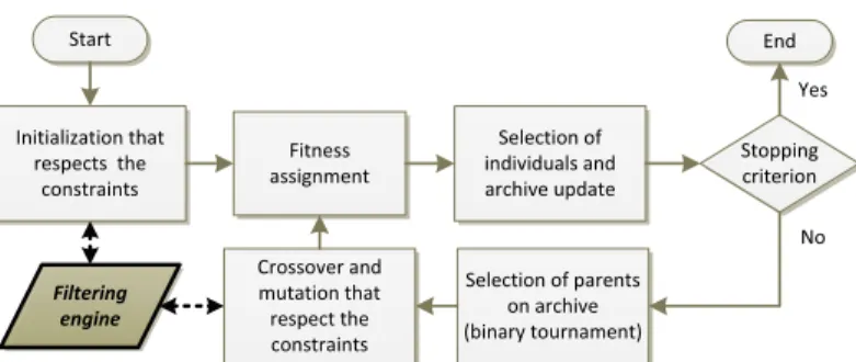
The CFB-EA algorithm we use belongs to the last kind of approach, which allows only feasible solutions in the archive. It is based on SPEA2 (Zitzler, Laumanns, and Thiele2001). The main ideas of SPEA2 are (a) the evaluation of a solution takes Pareto-dominance and the local density of solutions into account, (b) a set of the best and most diversified solutions are preserved in a separate archive, (c) there is a binary tournament in the archive to select parents for a crossover. In order to define CFB-EA, SPEA2 is updated with the addition of some constraint filtering that prunes the search space and prevents inconsistent solutions in the population during a) the initial population generation process, (b) the crossover and mutation process. Six parameters are required: size of the archive, size of the population, number of generations or any stopping criterion, crossover probability for individual selection, mutation probabilities for individual and gene selections. The CFB-EA algorithm is presented in Figure1in bold dark grey, with initial SPEA2 in light grey.
2.2. Possible improvements to the EA and computation time reductions
Experiments were conducted on the previous CFB-EA algorithm and compared to a Feasibility Rule algorithm and a Branch-and-bound (Pitiot, Aldanondo, and Vareilles2014). They were carried out using different problem sizes, from 105to 1016
solutions, and different constraint levels, with a ‘constrained solutions/unconstrained solutions’ ratio from 10−1 to 10−5. Logically, Branch-and-bound were discarded when solution space was over 106 with lower constrained problems or a
Figure 1. CFB-EA algorithm (Pitiot et al.2013).
constraint level higher than 10−2. CFB-EA and Feasibility rules were rather similar and computation time ranged between
2000 and 50,000 s, mainly in correlation with the problem size. This computation time was obtained with one CPU core, and the time could be divided by the number of used CPU cores to obtain the real computation time, thanks to the CFB-EA parallelisation possibilities of filtering engines.
As previously said, if waiting for one and, in some cases, more than ten hours of computation time may not be a problem in some situations, reducing computation time undoubtedly allows companies to be more reactive when deal-ing with a customer. Therefore, reducdeal-ing this computation time is the goal of this article for the CFB-EA algorithm and, more generally, for any EA algorithm that handles constraints. The CFB-EA algorithm shows a conventional behavior similar to most population-based optimisation approaches and most EAs: after an initial fast improvement (due to the fitness function that maximises solution dispersion on the Pareto front), performance stagnates before slowly coming closer to optimal values. A challenging aim is thus to find a way to avoid the previous stagnation sub-step. Given this purpose, two kinds of approaches, both of which are multi-stage, can be investigated. The first stage is almost always an EA, while the second stage can be either a similar EA or another technique, which is most often a Stochastic Local Search (SLS).
SLS algorithms (Hoos and Stützle2004) move from solution to solution in the search space by applying local changes until they find a supposed optimal solution or reach a time bound. In multi-objective contexts, the idea of mixing population-based approaches with an SLS algorithm is to benefit from both the quick and global improvements of the first EA and then use the SLS algorithm to improve search around found solutions. It leads to a well-converged and diversified final result (Blot, Kessaci, and Jourdan 2018). While our current proposals do not follow these ideas, they are clearly on our list of future research works.
The idea around EA-based multi-stage optimisation is to avoid tackling the whole problem size and complexity in a single shot. Two kinds of ideas can be found in the literature. The first ones try to reduce the number of criteria in a single optimisation shot with some kind of criteria distribution or association to different optimisation stages. The second ones try to reduce the size of solution spaces in a single optimisation shot with some kind of solution space decomposition and allocation to optimisation stages. For example, (Ascione et al.2016) distribute optimisation criteria in a three-stage optimisation approach in a study of energy retrofitting of hospital buildings. A similar approach can be seen in (Hamdy, Hasan, and Siren2013), also for building optimisation. Dealing more with solution space decomposition (Ji, Yu, and Zhang
2017) suggest using feasibility rules to quickly find a valid part of the solution space, then, once a solution is found, the investigated solution space is expended thanks to coevolution. Of course, approaches mixing criteria and solution space distribution can be found.
Some authors consider a large number of stages and speak of interactive methods (López Jaimes and Coello Coello
2013). These methods collect user preferences and give the possibility for the user to be active during the solution search process. This gives the user the opportunity to learn about the problem while exploring the available solutions (Miettinen, Ruiz, and Wierzbicki2008). This idea has been exploited in scalarization-based methods, such as (Linder, Lindkvist, and Sjoberg2012) or (Monz et al.2008). It has also been used with an evolutionary algorithm (Sinha et al.2014; Bechikh et al.
2015). Both approaches have some drawbacks, depending on the size and complexity of the problem (nature and number of objective functions). Three types of specifying preference information were identified by (Miettinen, Ruiz, and Wierzbicki
2008): trade-off information, reference points and classification of objective functions. Our approach follows the idea of trade-off information by delimiting an area in the search space. But it does not belong to the interactive method class, in the sense that it only interacts once with the user.
Figure 2. Proposed two-stage optimisation process.
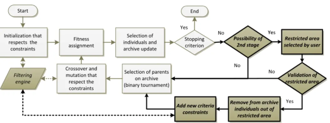
Figure 3. CFB-EA+ algorithm.
2.3. A proposal to reduce computation time for the CPPC problem: CFB-EA+
Within previous non-interactive methods, the partitioning of criteria or solution spaces and their affectation to a different optimisation two-stage means that before launching the optimisation, the user needs to have a priori preferences about the importance of the criteria, as well as knowledge of the solution space areas to investigate. As CFB-EA allows all criteria to be considered over the whole solution space, a key idea of the proposal is to avoid the need for these a priori blind preferences by showing the user a first Pareto of solutions that consider the whole problem. Then, given this Pareto knowledge, the user can decide on how to compromise between criteria and solution space.
Consequently, our proposal, called CFB-EA+ , mixes both solution space and criteria partitions but only when knowing a little about the solution space. The idea is to launch a first optimisation stage on the whole solutions space while taking into account all criteria, and to stop this process once a first ‘raw’ Pareto front can be identified at a time called switching time (ST). This Pareto result is shown to the customer in order for him/her, knowing the first general tendency of optimal compromise solutions space, to select a multi-criteria restricted area matching his/her criteria expectations.
A key point of CFB-EA+ is that optimisation criteria must be formalised as a numerical constraint that can be prop-agated. These numerical constraints are added to the CPPC configuration constraint model. Therefore, each assignment of any variable of the CPPC problem propagates towards a criteria value. Conversely, for our second optimisation stage, these numerical constraints are bounded with maximum values that correspond to the restricted area that fits customer expec-tations. Consequently, the two CFB-EA steps that are subject to constraint filtering (Section 2.1), individuals crossover and individuals mutation, respect these criteria bounds. As a result, the proposed second stage of the CFB-EA+ generates individuals that respect customer criteria restriction expectations.
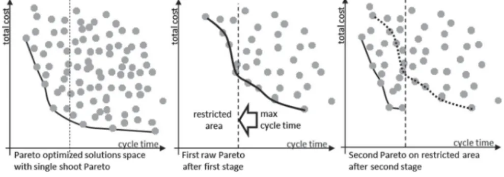
This two-stage optimisation process is illustrated in Figure2. On the left, the conventional single-stage optimisation that takes a long time. In the center at the switching time, a first raw Pareto, resulting from the first-stage optimisation on the whole solution space, that allows customer preferences to be captured (here the restricted area matching customer expectations is a maximum cycle time). On the right, the final Pareto on the previously restricted area.
The CFB-EA algorithm described in Figure1is updated as follows. Following the stopping criterion test step: (1) a switching time test is added, if the user is satisfied with the raw Pareto and has decided on a restricted area to investigate, (2) criteria constraints are inputted, (3) archive individuals that do not respect criteria constraints are removed, (4) criteria constraints are added to the filtering engine. The resulting CFBEA+ flowchart is shown in Figure3, with new steps in bold dark grey. The problem of the tuning of the switching time test will be addressed in the evaluation section at the end of Section (3.2).
Figure 4. Different elementary requirements: different solution spaces.
2.4. Interests and limits of CFB-EA+ The three following interests can be underlined.
Firstly, globally our idea corresponds to some kind of criteria ordering, but in this case, ordering is declared once a global tendency of solutions distribution with respect to criteria is known by the user. This means that CFB-EA+ avoids the ‘blind choice’ about criteria of other two-stage optimisation approaches that rely on a priori criteria ranking.
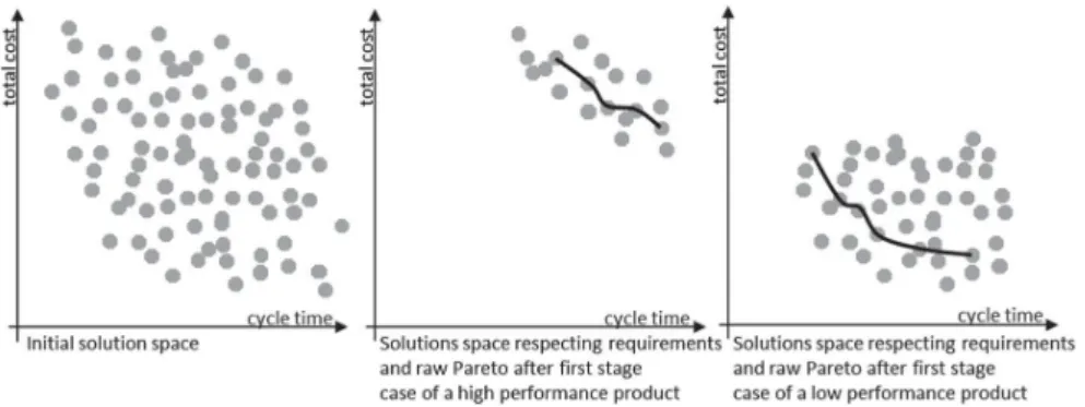
Secondly, the first optimisation stage is identical to CFB-EA, but the second one does not restart from scratch. In fact, it benefits from the first-stage individuals that respect the restricted area and that are systematically included in the initial population of the second optimisation stage. Thus there is no loss of computation time between the two optimisation stages. Thirdly, we have seen in Section 1.3 that, depending on the quantity of elementary requirements, the size of the problem to optimise can vary. Furthermore, according to the content of these elementary requirements (high or low product perfor-mance, for example, that essentially drives cost and cycle time), the requirement-respecting solution space that needs to be optimised can be clearly located in a different space area. This is shown in Figure4, where two kinds of requirements are shown, namely high and low product performance. As CFB-EA+ provides a general tendency before asking for criteria preference, any kind of customer requirements can be easily handled even if the interesting solution locations are very different.
Two limitations must be discussed.
The first limitation concerns the second stage of CFB-EA+ that can work only if each criterion can be formalised as a numerical constraint supporting filtering in any direction. When a numerical constraint can be written with a mathematical formula, f(x1, x2 . . .xn) (= > < ) 0, bound consistency proposed by (Lhomme1993) and interval arithmetic (Moore1966)
will guarantee that filtering techniques operate correctly, as long as the following conditions are fulfilled: • constraint expressed as (1) can be projected on any variable xi, meaning that a function fiexists as (2),
f (x1, x2. . .xn)= 0 (1)
xi= fi(x1, x2. . .xi−1, xi+1, . . . xn), (2)
• each projections fiis continuous and monotonous.
This is not a problem for simple computation but it can be delicate in some cases, as for example in energy-efficiency computations that have complex criterion computation that can’t be projected.
The second limitation concerns backtracking. As constraint filtering is not powerful or strong enough, when the restricted area corresponds to too hard constraints, the constraint filtering process of the two CFB-EA specific steps (individuals crossover and individuals mutation) can reach inconsistencies. By this, we mean that no solution remains for a configuration CSP variable during crossover or mutation. Thus, some backtrack processes are necessary to repair the solution. As this can also occur with CFB-EA, such a mechanism has been included in CFB-EA. But if without optimisation, the backtrack is not frequent at all, with optimisation and criteria constraints that are stronger, the optimisation process can spend a long time on backtracking. The experimentations of Section 3 will show that backtrack is from 10 to 40 times more frequent with CFB-EA+ .
2.5. Tuning CFB-EA+ parameters
In order to use CFB-EA+ , some recommendations relevant to the tuning of two parameters must be proposed. We first define and discuss the tuning parameters then propose some recommendations that will be validated according to the result
Figure 5. Different restricted areas for second the optimisation stage.
of the last experimentation section. The two parameters are the ‘switching time’ between the two optimisation stage and the ‘restricted area’ matching customer expectations when reducing optimisation search space.
About the switching time:
• With a too early switching time, the first optimisation stage might be unable to provide a rough Pareto sufficiently detailed to allow capturing a suitable restricted area matching customer expectations.
• At the opposite, with a too late switching time, the first optimisation stage will be very close to the optimal value and the computation time reduction will be rather low.
About the restricted area matching customer expectations:
• With a too large restricted area, the second optimisation stage will have a large solution space to investigate and, as before, the computation time reduction will be rather low.
• At the opposite, with a too small one, additional constraints on objectives will be stronger and thus many backtracks will be necessary to get individuals, reducing the convergence time.
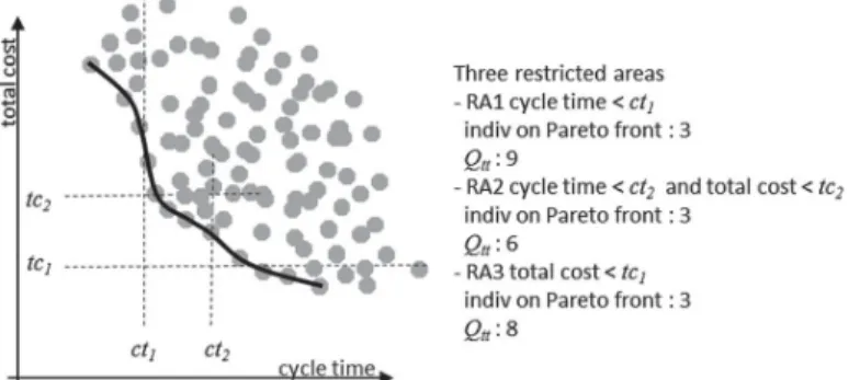
These two tuning parameters are more or less linked. Let us first consider the restricted area. Once the switching time is reached, the raw Pareto front is shown to the user and the idea is to ask him/her, knowing current criteria values, about a solution tendency. By solution tendency, we mean for two criteria to indicate either a preference on a single criterion or a compromise between the two criteria. This provides three criteria tendencies for reducing the search space and relevant restricted areas (RA 1, RA 2 and RA3), as shown in Figure5:
• RA 1 with single criterion cycle time < ct1,
• RA2 with compromise between cycle time < ct2and total cost < tc2,
• RA3 with single criterion total cost < tc1.
Thus as a suggestion, the raw Pareto front could be divided into three parts containing a same number of individuals (for example 1/4 of Pareto front that gathers 3 or 4 points each in Figure5). This is an order of magnitude suggestion and of course, it is possible to deviate from this solution according to customer expectations. Once this restricted area has been defined, another key-point linked to both parameters is the quantity of individuals existing in the selected area (noted Qtt) at
the switching time. If it is too low, it may result in a lack of diversity that will lead to local optimal convergence. This value will be quantified according to further experimentations. If it is not, this means that the switching time is too early and that the first optimisation stage must be continued or that the size of the constrained area should be increased.
3. Experimental evaluation of CFB-EA+
We will first deal with the experimentation metrics. Then we describe our main experimentations plan, present the associated result and discuss them. Then we propose some recommendations for using and tuning CFB-EA+ . Then with a larger model, we discuss scalability issues.
3.1. Metrics for experiments
As we want to characterise the optimisation computation time, we shall compute and follow the evolution, with respect to computation time, of the hypervolume HV metric defined by (Zitzler and Thiele1998). This measures the hypervolume
Figure 6. Hypervolume with the two criteria time and cost (Pitiot, Aldanondo, and Vareilles2014).
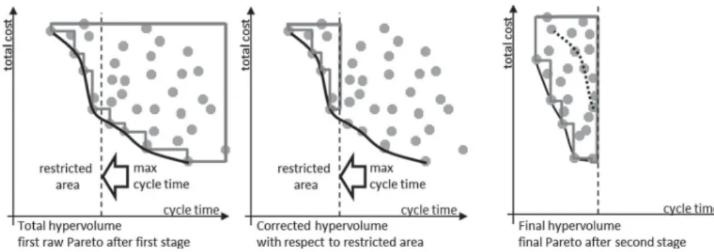
Figure 7. Hypervolume computation for CFB-EA+ .
dominated by a set of individuals, as shown in Figure6, where two criteria are considered and the HV is the surface inside the grey solid line. HV is maximum when solutions are most diversified on the Pareto front.
Given this definition, when evaluating CFB-EA+ we must correct the value of the hypervolume with respect to the switching time (ST) between the two optimisation stages and the associated restricted area. This means that once the two-stage optimisation is over when plotting the HV versus computation time:
• before switching time, we consider a corrected hypervolume as shown in the center of Figure7, which means that we discard all individuals outside the restricted area when computing HV,
• after switching time, as the constraints corresponding to the restricted area are respected by any individual, HV is unchanged, as shown on the right of Figure7.
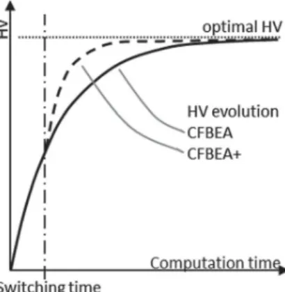
In order to be able to compare CFB-EA with CFB-EA+ on a given restricted area, the hypervolume relevant to CFB-EA will be computed with the CFB-EA+ mode used before switching time, meaning that HV computation will not consider individuals outside the restricted area. Thus, before switching time the HV time evolution is formally similar for both algorithms, then after switching time a different behavior should be observable, as shown in Figure8.
The main experimentations in order to compare CFB-EA and CFB-EA+ will be achieved with one main problem size. Then a larger problem will be considered to show the scalability of the proposal. By problem size, we mean the number of variables (n) where the customer can express an elementary requirement and the average number of possible values (p) for each. When constraints are not considered, the solution space size equals pn. When constraints are considered, the solution
space is reduced with respect to the constraint level, the ratio of the number of constrained solutions (c) divided by the number of unconstrained solutions (u). One should be aware that a high level corresponds to a low constrained problem. Thus constrained solution space size equals pn* c/u.
3.2. Experiments and results: comparing CFB-EA and CFB-EA+
These comparisons are made on a main problem that considers 30 variables (n= 30) with 6 values (p = 6). These 30 configuration variables correspond to 24 product variables (three sub-systems of 13, 6 and 5 configuration variables) and 6 process variables (three production operations of 2 configuration variables). Configuration constraints link between 2 and 4 variables and for each constraint, the ratio c/u is between 0.01 and 0.6. The goal of this section is to compare the computation times and the final hypervolume values of CFB-EA+ and CFB-EA. In order to avoid case dependency, the problems used
Figure 8. Comparing the HV evolution of CFB-EA+ and CFB-EA.
in these experiments are drawn from an analysis of CPPC problems (Pitiot et al.2016). This analysis is based on the notions of generic product modules, generic process operations, configuration patterns, and constraint patterns. It allows various CPPC problems to be generated.
3.2.1. Experimentation plans
First, CFB-EA reference results are obtained as follows:
(1) the CFB-EA algorithm is launched 10 times with a time bound of 9000 s,
(2) the average values of the first (HVfirst) and final (HVfinal) hypervolume are computed, (3) the average time to reach HVfinal is also noted. It might be below 9000 s.
It is important to note that these previous values consider the whole CFB-EA solution space. Then, considering the Pareto front associated with the previous HVfinal, and in order to achieve comparisons with CFB-EA+ :
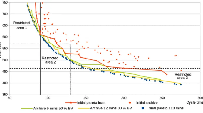
(4) three restricted areas (RA) illustrated in Figure9are defined as:
• RA1: cycle time < ctmax, ctmaxdefined with 25% individuals on Pareto front,
• RA2: cycle time < ctmed& total cost < tcmeddefined with 25% individuals on Pareto front
• RA3: total cost < tcmax, tcmaxdefined with 25% individuals on Pareto front.
(5) and for each restricted area:
• the corrected area hypervolume of CFB-EA (noted Hypervolume best value or (BV) in the results tables) is computed,
• the time to reach 95%, 99%, 99.9% and 100% of previous CFB-EA best value is also computed.
For each of these times and HV values, an average and a relative standard deviation (RSD) are provided. It can be seen in Figure9that in 12 min the Pareto front gives a good idea of possible potential compromises.
In order to avoid absolute values for switching times, the analysis is conducted with three switching times related to different levels of Hypervolume for each previously defined restricted area. These three switching times correspond to a HV value of 70, 80 and 90% of (HVfinal– HVfirst). They correspond roughly to 466, 800 and 1160 s. Each of these times is
associated with a number of individuals for each restricted area (Qttnoted ‘Qtt ind area’ in the tables of results), that have
been generated since the first computation and that are in the restricted area, including, of course, those that belong to the Pareto front.
For each couple (restricted area, switching time), CFB-EA+ is launched ten times with the same time bound of 9000 s, and the following values are recorded:
• the average of the previous number of individuals (Qtt),
• the times when the hypervolume reaches 95%, 99%, 99.9% and 100% of the hypervolume best value (BV) of CFB-EA,
Figure 9. Four restricted areas for CFB-EA+ .
As before, both the average and the RSD are provided for these times and HV values. These results are compared to the results provided by CFB-EA on the same restricted area with a gap percentage, 100 * [value (CFB-EA) – value (CFB-EA+ )] / value (CFB-EA).
Having conducted CFB-EA optimisation with various problem sizes, we came to the conclusion that the adequate size of the archive is 100, adequate population size is 150, appropriate crossover probability for individual selection is 0.8, and mutation probabilities for individual and gene selections should be set respectively at 0.5 and 0.1.
3.2.2. CFB-EA and CFB-EA+ comparison results and discussions
The hypervolume evolutions are shown and computation times are compared for the three restricted areas.
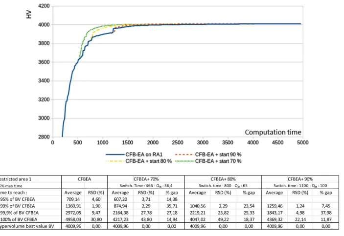
3.2.2.1. Restricted area 1, cycle time constraint. Figure10shows the hypervolume evolution on a graph with a table that details the computation times.
For any switching time and any time target (95%, 99%, 99.9%, and 100% and BV ) CFB-EA+ computation times are always lower, with a gap between 7% and 38%. For CFB-EA+ , as switching time 80% (800 s.) and 90% (1100 s.) are higher than CFB-EA time to reach 95% of BV CFB-EA (607 s.), there is no computation time comparison. It can be noticed that each of the ten runs reaches the hypervolume best value (BV 4009.96 with RSD= 0). Furthermore, even if CFB-EA + take more time to build individuals (CFB-EA+ backtrack rate by an individual is around 4.25%, while CFB-EA backtrack rate is close to 0.4%), it reaches BV more quickly.
3.2.2.2. Restricted area 2, compromise on cycle time and total cost constraint. Results are shown in Figure11.
These results show some interesting behavior. This restricted area is the most highly constrained one. The backtrack rate by an individual is around 17% (more than 40 times more than CFB-EA). It also has the lowest quantity of individuals from the first stage (respectively 20.4, 51.8 and 88.4). That leads to, with early switching times (70% and 80%) CFB-EA+ is unable to reach 99.9% and 100% of CFB-EA best value. However, those final values are very close to the hypervolume best value and they are reached very early. Moreover, all other values show lower computation times with gaps between 14% and 37%. Even if individuals are more difficult to obtain, due to backtracking, CFB-EA+ outperform CFB-EA. The keypoint would be to avoid the lack of diversity in the initial population that leads to local optimal for some cases of the earliest switching time.
Figure 10. Comparison CFB-EA+ with CFB-EA on restricted area 1.
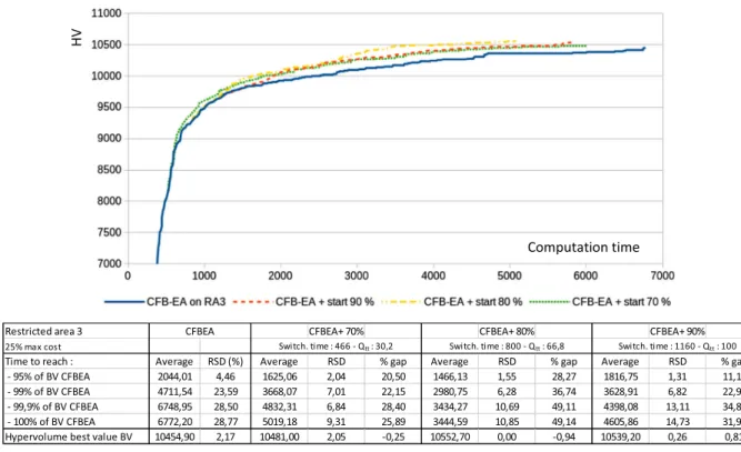
Figure 12. Comparison CFB-EA+ with CFB-EA on restricted area 3.
3.2.2.3. Restricted area 3, total cost constraint. Results are shown in Figure12.
For this restricted area, the tendency is similar. The backtrack rate by an individual is around 1,7%. The CFB-EA+ computation times are still always better than CFB-EA with values between 11% and 49%. The highest decreases are obtained with the intermediate switching time (80%) that also provides the best hypervolume value (10552.70).
3.2.2.4. Global results comparison. Table1gathers all computation time reductions as a percentage decrease with respect to various combinations of restricted areas and switching times.
When globally comparing all optimisation computation times, we obtain 30 times gaps: 10 with RA1, 8 with RA2 and 12 with RA3. The average of these 30 gaps is 27.05%, meaning that CFB-EA+ allows a significant reduction in computation time.
When comparing reductions with respect to restricted areas, the average gap of RA1 is 21.68%, while RA2 is 29.19% and RA3 is 30.09%, meaning that CFB-EA+ computation time reductions are a little higher when restricted areas are more constrained by total cost.
When considering only the time required to obtain the best hypervolume value (100% of BV CFB-EA), CFB-EA+ is always better than CFB-EA, with an average gap around 26% (excluding restricted area 2 with 70% and 80% switching time). This result, close to the global one (27.05), shows that significant computation time reductions are obtained with CFB-EA+ without any reduction of optimality level of the solutions.
When taking into account the different switching times, average gaps are as follows: CFB-EA+ 70%: 25.87%, CFB-EA+ 80%: 33.39% and CFB-EA + 90%: 22.93%. This means that the highest computation time reductions are provided with the intermediate switching time associated with a hypervolume equal to 80% of (HVfinal – HVfirst).
As previously mentioned, the quantity of individuals respecting the restricted area at the switching time (Qtt noted
‘Qtt ind area’ in the tables of results) at the beginning of the second CFB-EA+ optimisation stage must be considered as a switching time condition to avoid local optimums. Considering Table1, we suggest a minimum quantity of 60 for all restricted areas. This quantity of individuals will be the basis for our tuning recommendation. Of course, this quantity is roughly related to the size of the archive, which is 100 in previous experiments.
Table 1. Time reductions with respect to restricted areas and switching times.
CFBEA+ 70% CFBEA+ 80% CFBEA+ 90% % Gap average Computation times comparisons Switch. time: 325 s Switch. time: 800 s Switch. time: 1100 s wrt restricted area Restricted area 1: 25% max time Qtt: 36,4 Qtt: 65 Qtt: 100
Time to reach: % gap % gap % gap 95% of BV CFBEA 14,38
99% of BV CFBEA 35,71 23,54 7,45 All times to reach 99,9% of BV CFBEA 27,18 25,33 37,98 21,68 100% of BV CFBEA 14,94 18,37 11,87 15,06 % Gap average (Rest. area and
Swithching time)
23.05 22.41 19,10
Restricted area 2: 25% max time and max cost
Qtt: 20,4 Qtt: 51,8 Qtt: 88,4 Time to reach: % gap % gap % gap
95% of BV CFBEA 33,39 32,64 14,06
99% of BV CFBEA 36,15 37,36 32,22 All times to reach
99,9% of BV CFBEA 19,73 29,19
100% of BV CFBEA 28,01 28,01
% Gap average (Rest. area and Swithching time)
34,77 35,00 23,51
Restricted area 3: 25% max cost Qtt: 30,2 Qtt: 66,8 Qtt: 100 Time to reach: % gap % gap % gap
95% of BV CFBEA 20,50 28,27 11,12
99% of BV CFBEA 22,15 36,74 22,98 All times to reach 99,9% of BV CFBEA 28,40 49,11 34,83 30,09 100% of BV CFBEA 25,89 49,14 31,99 35,67 % Gap average (Rest. area and
Swithching time)
24,23 40,81 25,23
% Gap average wrt swithching time
25,87 33,39 22,93 % Gap avearge global 27,05
3.3. CFB-EA+ tuning recommendation for switching time and restricted area
The recommendation process works in the following way: once the first CFB-EA+ optimisation stage is launched on the whole solution space, at each loop, the possibility for a CFB-EA+ second stage initialisation is checked as follows:
• the individuals of the Pareto front are analyzed, and the constraints associated with each restricted area are computed, with respect to a 25% minimising of each criterion and 25% of central compromise of the two criteria, • the quantity of individuals included in each restricted area since the beginning of the CFB-EA + stage is calculated, • for each restricted area:
• if this quantity of individuals is smaller, the CFB-EA + first stage carries on,
• if this quantity of individuals is larger than 60 (given the archive is around 100 in our case), the process proposes to the user to launch the second CFB-EA+ optimisation stage,
• if the user is not satisfied by the proposed restricted area, CFB-EA first stage carries on,
• if the user is satisfied by the proposed restricted area, he can either validate the proposed restricted area or slightly modify it, as long as the minimum quantity is respected.
This recommendation will be used for optimising the larger problem of the next section. The initial CFB-EA+ algorithm shown in Figure3Section 2.3 is updated and gives the final CFB-EA+ algorithm that works as illustrated in Figure13. 3.4. Experiments with a much larger model and scalability issues
In order to deal with scalability issues, we consider now a CPPC problem of 60 variables (n= 60), with a similar number of values (p= 6) and constraint c/u ratio (between 0.01 and 0.6 for each constraint). The sixty configuration variables correspond to 46 product variables (one main subsystem of 22 variables plus four small subsystems of 6 variables) and 14 process variables (7 production operations). The archive size is larger, 150 (instead of 100), and the number of individuals that triggered the CFB-EA+ second stage initialisation possibility is set to 100 for all restricted area. The resulting switching times are, for RA1: 13736, for RA2: 7835 and for RA3: 8901. Figure14shows the hypervolume evolution for each restricted area with tables showing computer time reductions.
Figure 13. CFB-EA+ algorithm including the tuning process.
Figure 14. Comparison CFB-EA+ / CFB-EA with a larger model.
These curves and time reductions show that CFB-EA+ still works fine with larger problems. Furthermore, it can be noticed that the computation time reductions are globally larger with this 60-variables model (around 54%) compared to the 30-variables model described in the previous section (around 27%). This leads us to the conclusion that the interest of CFB-EA+ is greater when the size of the problem is larger. This size depends on the size of the initial CPPC problem but also on the quantity of elementary requirements provided by the customer. A large CPPC problem with a large quantity of elementary requirements can lead to a small problem to optimise. Thus, for our interactive configuration problem, if requirements are very detailed and cover almost all configuration variables, our recommendation would be to just use the CFB-EA single-stage approach and not CFB-EA+ .
4. Conclusions
The aim of this article was to reduce the optimisation computation time of a multi-criteria Concurrent Product and Process Configuration problem.
First the CPPC problem and the way to model it as a constrained satisfaction problem were recalled. Then optimisation was introduced with a brief survey of existing approaches and the existing CFB-EA algorithm recalled. Different approaches for reducing EA algorithm computation times were discussed and our proposal, CFB-EA+ described.
The key idea of CFB-EA+ is to avoid processing the whole solution space, but also to avoid a priori ordering of criteria and problem variables. The idea is to quickly compute in a first stage a first solution Pareto front and, in the knowledge of
this solution, to suggest some restricted areas to the user which will be subject to further enforced investigations in a second stage. As the CPPC problem and its optimisation criteria are modeled as a constraint satisfaction problem, this requires the identification and inclusion of the constraints corresponding to the restricted area to the first optimisation stage model in order to obtain the second stage optimisation model.
The following questions were addressed: does CFB-EA+ significantly reduce computation time? how can the CFB-EA+ switching-time and restricted-area tuning parameters be adjusted? does CFB-EA + work well with larger models?
With regard to computation time reductions, a low-constrained model of 30 configurable variables was used for exper-iments with various switching times and restricted areas. Without any parameter classification, a decrease in the order of magnitude of 30% of computation time can be expected. It has also been noted that this improvement is obtained without any decrease of the optimality level of the solutions.
For tuning the CFB-EA+ parameters, previous experiments have confirmed that the largest reductions in computation time were obtained with an intermediate switching time. But as a switching time associated with a small restricted area could lead to an over-constrained problem or a lack of diversity in the initial population, the quantity of individuals in a given restricted area has been preferred as a necessary tuning parameter. Given these results, we have proposed an updated version of CFB-EA+ that enables to suggest to the user switching times associated with a restricted area with respect to a criterion tendency (cost constraint, duration constraint, compromise between the two criteria). Further works must be undertaken in order to refine parameter tuning according to user criteria tendency, model size, model constraint level, and archive size.
In answer to the question of whether CFB-EA+ works well on a larger scale, a model gathering 60 variables with char-acteristics similar to the previous one was also considered. Experiments confirmed previous computation time reductions and show even better results for a larger model.
These conclusions clearly show the interests of the CFB-EA+ approach in reducing optimisation computation times. Furthermore, considering company expectations, and especially in B2C configuration situations, the possibility of showing a first Pareto Front in less than 15 min, and thus providing an idea of the solution space distribution will undoubtedly serve to keep the customer’s attention focused on the configuration solution possibilities. By viewing this Pareto, the customer can express a well-founded expectation of his criteria preferences and therefore feel greater satisfaction. For B2B situations, the contribution is a little different, as the customer usually has to wait for an optimal solution, which takes quite a long time. Here, even if this computation time is significantly reduced, it is possible to provide the customer with partial solution-space tendencies in a relatively short time, thus limiting the search for optimal space regions.
These results have been obtained thanks to six assumptions or limitations: a discrete definition domain for configuration variables, a production process as a sequence of operations, two conflicting criteria, an infinite capacity of the resources for process configuration, optimisation criteria formalised as a numerical constraints and a low backtracking need. The first three assumptions are not strong constraints; they were just made for the simplicity of the models and associated computa-tions. Infinite capacity of the resource in process configuration is not a hard hypothesis, because most companies launching production in a ‘configuration to order mode’ are flexible enough to adapt their capacities according to the demand. At the opposite, optimisation criteria must be formalised as numerical constraints supporting filtering in any direction. This is the key requirement and the single strong limitation of the contribution of this paper. If this is not the case, it is not possible to launch the second optimisation stage, as area restrictions formalised with constraints will not be able to prune individual optimisation candidates. The last limitation, backtracking, exists in any constrained problem optimisation: when constraints become heavier, it is harder to find solutions.
In terms of future work, we have already mentioned CFB-EA+ parameter tuning and coupling CFB-EA with stochastic local search. As this article has addressed two-criteria problems, we think that moving to three criteria should also be inves-tigated. A delicate issue here may be to express the constraints that characterise three-dimensional restricted areas. The last work perspective concerns the possibility of using the CFB-EA+ key idea, two similar optimisation stages differentiated by the addition of criteria constraints on the problem, with other multi-evolutionary algorithms. For this last question, we have good confidence that the proposed idea should work fine with any multi-objective and constrained evolutionary algorithms.
Disclosure statement
No potential conflict of interest was reported by the authors.
References
Aldanondo, M., and E. Vareilles. 2008. “Configuration for Mass Customization: How to Extend Product Configuration towards Requirements and Process Configuration.” Journal of Intelligent Manufacturing 19 (5): 521–535.
Ascione, F., N. Bianco, C. De Stasio, G. Mauro, and G. Vanoli. 2016. “Multi-stage and Multi-objective Optimization for Energy Retrofitting a Developed Hospital Reference Building: A New Approach to Assess Cost-optimality.” Applied Energy 174: 37–68.
Bartak, R., M. A. Salido, and F. Rossi. 2010. “Constraint Satisfaction Techniques in Planning and Scheduling.” Journal of Intelligent
Manufacturing 21 (1): 5–15.
Bechikh, S., M. Kessentini, L. B. Said, and K. Ghedira. 2015. “Preference Incorporation in Evolutionary Multiobjective Optimization: A Survey of the State-of-the-art.” Advances in Computers 98: 141–207.
Bessiere, C. 2006. “Constraint Propagation.” Chap. 3 in Handbook of Constraint Programming, edited by Francesca Rossi, Peter van Beek, and Toby Walsh, 29–70. Amsterdam: Elsevier.
Blot, A., M. Kessaci, and L. Jourdan. 2018. “Survey and Unification of Local Search Techniques in Metaheuristics for Multi-objective Combinatorial Optimization.” Journal of Heuristics 24 (6): 853–877.
Campagna, D., and A. Formisano. 2013. “Product and Production Process Modeling and Configuration.” Fundamenta Informaticae 124 (4): 403–425.
Coello Coello, Carlos A., Gary B. Lamont, and David A. Van Veldhuizen. 2007. Evolutionary Algorithms for Solving Multi-objective
Problems (Genetic and Evolutionary Computation Series). New York: Springer.
Dou, R., C. Zong, and M. Li. 2016. “An Interactive Genetic Algorithm with the Interval Arithmetic Based on Hesitation and its Application to Achieve Customer Collaborative Product Configuration Design.” Applied Soft Computing Journal 38 (1): 384–394. Du Gang, Jiao Roger J., and Chen Mo. 2014. “Joint Optimization of Product Family Configuration and Scaling Design by Stackelberg
Game.” European Journal of Operational Research 232 (2): 330–341.
Felfernig, A., L. Hotz, C. Baglay, and J. Tiihonen. 2014. Knowledge-based Configuration from Research to Business Cases. Amsterdam: Morgan Kaufmann.
Fleischanderl, G., G. Friedrich, A. Haselböck, H. Schreiner, and M. Stumptner. 1998. “Configuring Large Systems Using Generative Constraint Satisfaction.” IEEE Intelligent Systems 13 (4): 59–68.
Hamdy, M., A. Hasan, and K. Siren. 2013. “A Multi-stage Optimization Method for Cost-optimal and Nearly-zero-energy Building Solutions in Line with the EPBD-recast 2010.” Energy and Buildings 56: 189–203.
Hoos, H., and T. Stützle. 2004. Stochastic Local Search-foundations and Applications. San Francisco, CA: Morgan Kaufmann.
Hotz, L., A. Felfernig, M. Stumptner, A. Ryabokon, C. Bagley, and K. Wolter. 2014. “Configuration Knowledge Representation and Reasoning.” Chap. 6 in Knowledge-based Configuration from Research to Business Cases, edited by Alexander Felfernig, Lothar Hotz, Claire Bagley, and Juha Tiihonen, 41–72. Amsterdam: Morgan Kaufmann.
Ji, J. Y., W. J. Yu, and J. Zhang. 2017. “A Two-stage Coevolution Approach for Constrained Optimization.” Proceedings of the Genetic and Evolutionary Computation Conference Companion, GECCO’17, Berlin, Germany, July 15–19, 167–168.
Junker, U. 2006. “Configuration.” Chap. 24 in Handbook of Constraint Programming, edited by Francesca Rossi, Peter van Beek, and Toby Walsh, 835–875. Amsterdam: Elsevier.
Karppinen, H., K. Seppänenand, and J. Huiskonen. 2014. “Identifying Product and Process Configuration Requirements in a Decentralised Service Delivery System.” International Journal of Services and Operations Management 17 (3): 294–310.
Konstantas, D., S. Ioannidis, V. S. Kouikoglou, and E. Grigoroudis. 2018. “Linking Product Quality and Customer Behavior for Perfor-mance Analysis and Optimization of Make-to-order Manufacturing Systems.” International Journal of Advanced Manufacturing
Technology 95 (1–4): 587–596.
Koubarakis, M. 2006. “Temporal CSPs.” Chap. 19 in Handbook of Constraint Programming, edited by Francesca Rossi, Peter van Beek, and Toby Walsh, 663–697. Amsterdam: Elsevier.
Lhomme, O. 1993. “Consistency Techniques for Numerical CSPs.” Proceedings of the International Joint Conference on Artificial
Intelligence IJCAI 93: 232–238.
Linder, J., S. Lindkvist, and J. Sjoberg. 2012. “Two Step Framework for Interactive Multi-objective Optimization.” Technical Report LiTH-ISY-R-3043, Department of Electrical Engineering, Linkoping University.
López Jaimes, A., and C. Coello Coello. 2013. “Interactive Approaches Applied to Multiobjective Evolutionary Algorithms.” Chap. 8 in
Multicriteria Decision Aid and Artificial Intelligence: Links, Theory and Applications, edited by Michael Doumpos and Evangelos
Grigoroudis, 191–208. West Sussex: Wiley-Blackwell.
Mailharro, D. 1998. “A Classification and Constraint-based Framework for Configuration.” Artificial Intelligence for Engineering Design,
Analysis and Manufacturing 12 (4): 383–397.
Mayer, W., M. Stumptner, P. Killisperger, and G. Grossmann. 2011. “A Declarative Framework for Work Process Configuration.” Artificial
Intelligence for Engineering Design, Analysis and Manufacturing 25 (2): 143–162.
Mezura-Montes, E., and C. Coello Coello. 2011. “Constraint-handling in Nature-inspired Numerical Optimization: Past, Present and Future.” Swarm and Evolutionary Computation 1 (4): 173–194.
Miettinen, K., F. Ruiz, and A. P. Wierzbicki. 2008. “Introduction to Multiobjective Optimization: Interactive Approaches.” In
Multiob-jective Optimization. Lecture Notes in Computer Science, Vol. 5252, edited by J. Branke, K. Deb, K. Miettinen, and R. Słowi´nski,
27–57. Berlin: Springer.
Mittal, S., and F. Frayman. 1989. “Towards a Generic Model of Configuration Tasks.” Proceedings of the Eleventh International Joint
Conference on Artificial Intelligence 2: 1395–1401.
Montanari, U. 1974. “Networks of Constraints: Fundamental Properties and Application to Picture Processing.” Information Sciences 7: 95–132.
Monz, M., K. Küfer, T. Bortfeld, and C. Thieke. 2008. “Pareto Navigation: Algorithmic Foundation of Interactive Multi-criteria IMRT Planning.” Physics in Medicine and Biology 53: 985–998.
Moore, Ramon E. 1966. Interval Analysis. Englewood Cliffs, NJ: Prentice Hall.
Pitiot, P., M. Aldanondo, and E. Vareilles. 2014. “Concurrent Product Configuration and Process Planning: Some Optimization Experimental Results.” Computers in Industry 65 (4): 610–621.
Pitiot, P., M. Aldanondo, E. Vareilles, P. Gaborit, M. Djefel, and S. Carbonnel. 2013. “Concurrent Product Configuration and Process Planning, towards an Approach Combining Interactivity and Optimality.” International Journal of Production Research 51 (2): 524–541.
Pitiot, P., L. Garcés Monge, E. Vareilles, and M. Aldanondo. 2016. “Benchmark for Configuration and Planning Optimization Problems: Proposition of a Generic Model.” Proceedings of the 18th International Configuration Workshop (within CP 2016 Conference), Toulouse, France, 89–96.
Sabin, D., and E. Freuder. 1996. “Configuration as Composite Constraint Satisfaction.” Proceedings of the AAAI 1996 Workshop on Configuration, 28–36. AAAI Press.
Sabin, D., and R. Weigel. 1998. “Product Configuration Frameworks – a Survey.” IEEE Intelligent Systems 13 (4): 42–49.
Schierholt, K. 2001. “Process Configuration: Combining the Principles of Product Configuration and Process Planning.” Artificial
Intelligence for Engineering Design, Analysis and Manufacturing 15 (5): 411–424.
Sinha, A., P. Korhonen, J. Wallenius, and K. Deb. 2014. “An Interactive Evolutionary Multi-objective Optimization Algorithm with a Limited Number of Decision Maker Calls.” European Journal of Operational Research 233 (3): 674–688.
Tang, D., Q. Wang, and I. Ullah. 2017. “Optimisation of Product Configuration in Consideration of Customer Satisfaction and Low Carbon.” International Journal of Production Research 55 (12): 3349–3373.
Tseng, H., C. Chang, and S. Chang. 2005. “Applying Case-based Reasoning for Product Configuration in Mass Customization Environments.” Expert Systems with Applications 29 (4): 913–925.
Van Beek, P. 2006. “Backtracking Search Algorithms.” Chap. 4 in Handbook of Constraint Programming, edited by Francesca Rossi, Peter van Beek, and Toby Walsh, 85–134. Amsterdam: Elsevier.
Wang, L., S. S. Zhong, and Y. J. Zhang. 2017. “Process Configuration Based on Generative Constraint Satisfaction Problem.” Journal of
Intelligent Manufacturing 28: 945–957.
Wei, W., W. Fan, and Z. Li. 2014. “Multi-objective Optimization and Evaluation Method of Modular Product Configuration Design Scheme.” International Journal of Advanced Manufacturing Technology 75 (9–12): 1527–1536.
Yadav, S. R., Y. Dashora, R. Shankar, F. Chan, and M. Tiwari. 2008. “An Interactive Particle Swarm Optimisation for Selecting a Product Family and Designing its Supply Chain.” International Journal of Computer Applications in Technology 31 (3/4): 168–186. Zhang, L., E. Vareilles, and M. Aldanondo. 2013. “Generic Bill of Functions, Materials, and Operations for SAP 2 Configuration.”
International Journal of Production Research 51 (2): 465–478.
Zheng, L. Y., H. F. Dong, P. Vichare, A. Nassehi, and S. T. Newman. 2008. “Systematic Modeling and Reusing of Process Knowledge for Rapid Process Configuration.” Robotics and Computer-Integrated Manufacturing 24 (6): 763–772.
Zheng, P., X. Xu, S. Yu, and C. Liu. 2017. “Personalized Product Configuration Framework in an Adaptable Open Architecture Product Platform.” Journal of Manufacturing Systems 43: 422–435.
Zitzler, E., M. Laumanns, and L. Thiele. 2001. “SPEA2: Improving the Strength Pareto Evolutionary Algorithm.” Technical Report 103, Computer Engineering and Communication Networks Lab (TIK). Swiss Federal Institute of Technology (ETH), Zurich.
Zitzler, E., and L. Thiele. 1998. “Multiobjective Optimization Using Evolutionary Algorithms – A Comparative Case Study.” In Parallel
Problem Solving from Nature – PPSN V. PPSN 1998. Lecture Notes in Computer Science, Vol. 1498, edited by A. E. Eiben, T. Bäck,