HAL Id: hal-00822973
https://hal.inria.fr/hal-00822973
Submitted on 28 Jun 2016
HAL is a multi-disciplinary open access
archive for the deposit and dissemination of
sci-entific research documents, whether they are
pub-lished or not. The documents may come from
teaching and research institutions in France or
abroad, or from public or private research centers.
L’archive ouverte pluridisciplinaire HAL, est
destinée au dépôt et à la diffusion de documents
scientifiques de niveau recherche, publiés ou non,
émanant des établissements d’enseignement et de
recherche français ou étrangers, des laboratoires
publics ou privés.
Handling Partitioning Skew in MapReduce using LEEN
Shadi Ibrahim, Hai Jin, Lu Lu, Bingsheng He, Gabriel Antoniu, Song Wu
To cite this version:
Shadi Ibrahim, Hai Jin, Lu Lu, Bingsheng He, Gabriel Antoniu, et al.. Handling Partitioning Skew in
MapReduce using LEEN. Peer-to-Peer Networking and Applications, Springer, 2013. �hal-00822973�
(will be inserted by the editor)
Handling Partitioning Skew in MapReduce using
LEEN
Shadi Ibrahim⋆ · Hai Jin · Lu Lu ·
Bingsheng He · Gabriel Antoniu · Song
Wu
Received: date / Accepted: date
Abstract MapReduce is emerging as a prominent tool for big data process-ing. Data locality is a key feature in MapReduce that is extensively leveraged in data-intensive cloud systems: it avoids network saturation when processing large amounts of data by co-allocating computation and data storage, partic-ularly for the map phase. However, our studies with Hadoop, a widely used MapReduce implementation, demonstrate that the presence of partitioning
skew1 causes a huge amount of data transfer during the shuffle phase and
leads to significant unfairness on the reduce input among different data nodes. As a result, the applications severe performance degradation due to the long data transfer during the shuffle phase along with the computation skew, par-ticularly in reduce phase.
In this paper, we develop a novel algorithm named LEEN for locality-aware and fairness-locality-aware key partitioning in MapReduce. LEEN embraces an asynchronous map and reduce scheme. All buffered intermediate keys are
par-⋆ corresponding author
Shadi Ibrahim, Gabriel Antoniu INRIA Rennes-Bretagne Atlantique Rennes, France
E-mail:{shadi.ibrahim, gabriel.antoniu}@inria.fr Hai Jin, Lu Lu, Song Wu
Cluster and Grid Computing Lab
Services Computing Technology and System Lab Huazhong University of Science and Technology Wuhan, China
E-mail: [email protected] Bingsheng He
School of Computer Engineering
Nanyang Technological University Singapore E-mail: [email protected]
1 Partitioning skew refers to the case when a variation in either the intermediate keys’
titioned according to their frequencies and the fairness of the expected data distribution after the shuffle phase. We have integrated LEEN into Hadoop. Our experiments demonstrate that LEEN can efficiently achieve higher local-ity and reduce the amount of shuffled data. More importantly, LEEN guar-antees fair distribution of the reduce inputs. As a result, LEEN achieves a performance improvement of up to 45% on different workloads.
Keywords MapReduce · Hadoop · cloud computing · skew partitioning ·
intermediate data;
1 Introduction
MapReduce [1], due to its remarkable features in simplicity, fault tolerance, and scalability, is by far the most successful realization of data intensive cloud computing platforms[2]. It is often advocated as an easy-to-use, efficient and reliable replacement for the traditional programming model of moving the data to the cloud[3]. Many implementations have been developed in different programming languages for various purposes [4][5][6]. The popular open source implementation of MapReduce, Hadoop [7], was developed primarily by Yahoo, where it processes hundreds of terabytes of data on tens of thousands of nodes [8], and is now used by other companies, including Facebook, Amazon, Last.fm, and the New York Times [9].
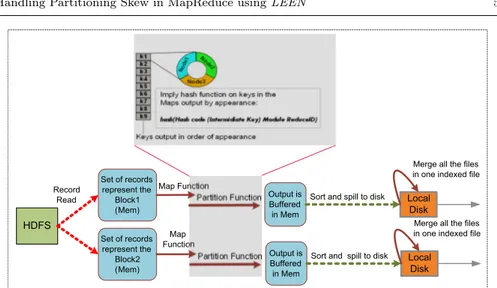
The MapReduce system runs on top of the Google File System (GFS) [10], within which data is loaded, partitioned into chunks, and each chunk replicated across multiple machines. Data processing is co-located with data storage: when a file needs to be processed, the job scheduler consults a storage metadata service to get the host node for each chunk, and then schedules a “map” process on that node, so that data locality is exploited efficiently. The map function processes a data chunk into key/value pairs, on which a hash partitioning function is performed, on the appearance of each intermediate key produced by any running map within the MapReduce system:
hash (hash code (Intermediate-Keys) module ReduceID)
The hashing results are stored in memory buffers, before spilling the in-termediate data (index file and data file) to the local disk [11]. In the reduce stage, a reducer takes a partition as input, and performs the reduce function on the partition (such as aggregation). Naturally, how the hash partitions are stored among machines affects the network traffic, and the balance of the hash partition size is an important indicator for load balancing among reducers.
In this work, we address the problem of how to efficiently partition the intermediate keys to decrease the amount of shuffled data, and guarantee fair distribution of the reducers’ inputs, resulting in improving the overall perfor-mance. While, the current Hadoop’s hash partitioning works well when the keys are equally appeared and uniformly stored in the data nodes, with the presence of partitioning skew, the blindly hash-partitioning is inadequate and can lead to:
1. Network congestion caused by the huge amount of shuffled data, (for exam-ple, in wordcount application, the intermediate data are 1.7 times greater in size than the maps input, thus tackling the network congestion by locality-aware map executions in MapReduce systems is not enough);
2. unfairness of reducers’ inputs; and finally
3. severe performance degradation [12] (i.e. the variance of reducers’ inputs, in turn, causes a variation in the execution time of reduce tasks, resulting in longer response time of the whole job, as the job’s response time is dominated by the slowest reduce instance).
Recent research has reported on the existence of partitioning skew in many MapReduce applications [12][13][14], but none of the current MapReduce im-plementations have overlooked the data skew issue[15]. Accordingly, in the presence of partitioning skew, the existing shuffle strategy encounters the prob-lems of long intermediate data shuffle time and noticeable network overhead. To overcome the network congestion during the shuffle phase, we propose to expose the locality-aware concept to the reduce task; However, locality-aware reduce execution might not be able to outperform the native MapReduce due to the penalties of unfairness of data distribution after the shuffle phase, result-ing in reduce computation skew. To remedy this deficiency, we have developed an innovative approach to significantly reduce data transfer while balancing the data distribution among data nodes.
Recognizing that the network congestion and unfairness distribution of reducers’ inputs, we seek to reduce the transferred data during the shuffle phase, as well as achieving a more balanced system. We develop an algorithm, locality-aware and fairness-aware key partitioning (LEEN ), to save the net-work bandwidth dissipation during the shuffle phase of the MapReduce job along with balancing the reducers’ inputs. LEEN is conducive to improve the data locality of the MapReduce execution efficiency by the virtue of the asynchronous map and reduce scheme, thereby having more control on the keys distribution in each data node. LEEN keeps track of the frequencies of buffered keys hosted by each data node. In doing so, LEEN efficiently moves buffered intermediate keys to the destination considering the location of the high frequencies along with fair distribution of reducers’ inputs. To quan-tify the locality, data distribution and performance of LEEN, we conduct a comprehensive performance evaluation study using LEEN in Hadoop 0.21.0. Our experimental results demonstrate that LEEN interestingly can efficiently achieve higher locality, and balance data distribution after the shuffle phase. In addition, LEEN performs well across several metrics, with different parti-tioning skew degrees, which contribute to the performance improvement up to 45%.
LEEN is generally applicable to other applications with data partitioning and this will result in guaranteed resource load balancing with a small overhead due to the asynchronous design. The main focus of this paper and the primary usage for LEEN is on MapReduce applications where partitions skew exists (e.g., many scientific applications [12][13][14][16] and graph applications [17]).
We summarize the contributions of our paper as follows:
– An in-depth study on the source of partitioning skew in MapReduce and its impacts on application performance.
– A natural extension of the data-aware execution by the native MapReduce model to the reduce task.
– A novel algorithm to explore the data locality and fairness distribution of intermediate data during and after the shuffle phase, to reduce network congestion and achieve acceptable data distribution fairness.
– Practical insight and solution to the problems of network congestion and reduce computation skew, caused by the partitioning skew, in emerging Cloud.
The rest of this paper is organized as follows. Section 2 briefly introduces MapReduce and Hadoop, and illustrates the recent partitioning strategy used in Hadoop. The partitioning skew issue is explored and empirically analyzed in sections 3. The design and implementation of the LEEN approach is discussed in section 4. Section 5 details the performance evaluation. Section 6 discusses the related works. Finally, we conclude the paper and propose our future work in section 7.
2 Background
In this section, we briefly introduce the MapReduce model and its widely used implementation, Hadoop. Then we briefly zoom on the workflow of job execution in Hadoop introducing side by side the map, reduce and partition functions.
2.1 MapReduce Model
The MapReduce [1] abstraction is inspired by the Map and Reduce functions, which are commonly used in functional languages such as Lisp. Users express the computation using two functions, map and reduce, which can be carried out on subsets of the data in a highly parallel manner. The runtime system is responsible for parallelizing and fault handling.
The steps of the process are as follows:
– The input is read (typically from a distributed file system) and broken up into key/value pairs. The key identifies the subset of data, and the value will have computation performed on it. The map function maps this data into sets of key/value pairs that can be distributed to different processors. – The pairs are partitioned into groups for processing, and are sorted ac-cording to their key as they arrive for reduction. The key/value pairs are reduced, once for each unique key in the sorted list, to produce a combined result.
Node 1 No de 2 Node3 k1 k2 k3 k4 k5 k6 k7 k8 k9
Keys output in order of appearance Imply hash function on keys in the Maps output by appearance:
hash(Hash code (Intermidiate Key) Module ReduceID)
HDFS Set of records represent the Block1 (Mem) Set of records represent the Block2 (Mem) Output is Buffered in Mem Local Disk Record Read Map Function
Partition Function Sort and spill to disk
Merge all the files in one indexed file
Output is Buffered in Mem Local Disk Map Function
Sort and spill to disk
Merge all the files in one indexed file Partition Function
Fig. 1 The workflow of the two phases in MapReduce job: the map phase and reduce phase
2.2 Hadoop
Hadoop [7] is a java open source implementation of MapReduce sponsored by Yahoo! The Hadoop project is a collection of various subprojects for re-liable, scalable distributed computing. The two fundamental subprojects are the Hadoop MapReduce framework and the HDFS. HDFS is a distributed file system that provides high throughput access to application data [7]. It is in-spired by the GFS. HDFS has master/slave architecture. The master server, called NameNode, splits files into blocks and distributes them across the clus-ter with replications for fault tolerance. It holds all metadata information about stored files. The HDFS slaves, the actual store of the data blocks called DataNodes, serve read/write requests from clients and propagate replication tasks as directed by the NameNode.
The Hadoop MapReduce is a software framework for distributed processing of large data sets on compute clusters [7]. It runs on the top of the HDFS. Thus data processing is collocated with data storage. It also has master/slave archi-tecture. The master, called Job Tracker (JT), is responsible of : (a) Querying the NameNode for the block locations, (b) considering the information re-trieved by the NameNode, JT schedule the tasks on the slaves, called Task Trackers (TT), and (c) monitoring the success and failures of the tasks.
2.3 Zoom on job execution in Hadoop
The MapReduce program is divided into two phases, map and reduce. For the map side, it starts by reading the records in the Map process, then the map function processes a data chunk into key/value pairs, on which the hash partitioning function is performed as shown in Fig 1. This intermediate result,
Node1 1 1 1 2 2 2 3 3 3 4 4 4 5 5 5 6 6 6 Node2 Node3 Key 1 Key 6 Key 5 Key 4 Key 3 Key 2
Best Case Worst Case
21 21 21
We assume balance map execution
(a) Keys’ Frequencies Variation
Node1 Node2 Node3 Key 1 Key 6 Key 5 Key 4 Key 3 Key 2
Best Case Worst Case
12 12 12 We assume balance map execution 4 1 1 1 4 1 1 1 4 3 2 1 1 3 2 2 1 3
(b) Inconsistency in Key’s Distribution Fig. 2 Motivational Example: demonstrates the worst and best partitioning scenarios when applying the current blindly key partitioning in MapReduce in the presence of Par-titioning skew. The keys are ordered by their appearance while each value represents the frequency of the key in the data node.
refereed as record, is stored with its associate partition in the buffer memory (100 MB for each map by default). If the buffered data reaches the buffer threshold (80% of the total size), the intermediate data will be sorted according to the partition number and then by key and spilled to the local disk as an index file and a data file. All files will be then merged as one final indexed file -by indexed we mean indexed according to the partition number that represents the target reduce. The reduce case is starting as soon as the intermediate indexed files are fetched to the local disk; the files from multiple local map outputs will be written at the same time (by default five pipes will be available for the different nodes). The files will be buffered in the memory in a “shuffle buffer”; when the shuffle buffer reaches a threshold the files will be redirected to the local disk, then the different files will be merged according to the user specific application, and merged files from the shuffle buffer will be tailed in the local disk. Finally the merged data will be passed to the reduce function and then the output will be written to the HDFS or elsewhere according to the user specific application.
3 Partitioning Skew in MapReduce
The outputs of map tasks are distributed among reduce tasks via hash par-titioning. The default hash-partitioning, however, is designed to guarantee evenly distribution of keys amongst the different data nodes, that is, if we have n data nodes and k different keys then the number of keys which will be partitioned to each data node isk
n, regardless of the frequencies of each distinct key (usually the number of records are associated with one key). The default hash-partitioning therefore is only adequate when the number of records asso-ciated with each key are relatively equal and the key’s records are uniformly distrusted amongst data nodes.
However, in the presence of partitioning skew the hash-partitioning as-sumption will break and therefore reduce-skew and network congestion can arise in practice[13][14][12] [18]. As we earlier stated the partition skew phe-nomena refereed to the case when the keys’ frequencies vary and/or the key’s records among data node are not uniformly distributed. Consider the two ex-amples which represent each factor separately:
– Keys’ Frequencies Variation: Although the partitioning function perfectly distributes keys across reducers, some reducers may still be assigned more data simply because the key groups they are assigned to contain signifi-cantly more values. Fig 2-a presents the first example considering three data nodes and six keys. We vary keys frequencies to 3, 6, 9, 12, 15, and18 records per key, accordingly using the blindly hash-partitioning which is based on the sequence of the keys appearance during the map phase, the distribution of reducers’ inputs will vary between the best partitioning: 21 records for each reducer, and the worst case partitioning: the input of the reducers in node1, node2, and node3 will be 9, 21 and 33 records respec-tively. Despite that in both cases the number of keys assigned to each data node is the same, two keys per node in our example.
Accordingly reduce-skew will occur, in our example, node3 will finish its reduce nearly four times slower than node1; consequently, heavy reduce execution on some nodes. Thus performance experiences degradation (i.e. waiting the last subtask to be finished), and less resource utilization (i.e. node1 will be idle while node3 is overloaded). [18] and [12] have demon-strated the existence of this phoneme in some biological applications, for example, [12] has demonstrated that because of the keys’ frequencies vari-ation, in CloudBurst [18] applicvari-ation, some reducers will finish their task four times longer than other reduces.
– Inconsistency in Key’s Distribution: As a second example, even when the keys have the same frequencies and therefore the partitioning function per-fectly distributes keys across reducers – all reducers inputs are relatively equal –. But, however, the blind hash-partitioning may lead to high network congestion, especially when the key’s recodes are not uniformly distributed among data nodes. Fig 2-b presents the second example considering three data nodes and six keys. All keys have the same frequents, 6 records per key but the key’s distribution is inconsistent among the nodes. Applying the blindly hash-partitioning will result with evenly reducers’s inputs, but the data transfer, in contrast with the total map output during the shuf-fle phase will vary from 41.6%1, in the best case, to 83.3% in the worst case. Accordingly network congestion during the shuffle phase is strongly depending on the hash-partitioning.
However, in the case of partitioning skew, when both factors, keys’ fre-quencies variation and inconsistency in key’s distribution, will occur the blind hash-partitioning may result will both skew-reduce and network congestion as demonstrated in section 5.
1 This value represents the ratio = transf erred data during shuf f le map phase output
Table 1 MapReduce Applications’ Classification
Map Only MapReduce with
Combiner
MapReduce without Combiner
Single Record Multi record
Distributed Grep
Wordcount Distributed Sort Wordcount without
Com-biner, Count of URL Access Fre-quency Graph processing [21], Machine Learning [20], Scientific application [18][16][19]
3.1 Partitioning Skew in MapReduce Applications
MapReduce has been applied widely in various fields including data- and compute- intensive applications, machine learning, and multi-core program-ming. In this sub-section we intend to classify the MapReduce application in term of skewed intermediate data.
A typical MapReduce application includes four main functions: map, re-duce, combiner and shuffle functions. Accordingly we could classify MapRduce applications in respect to the main applied function in these applications into: map-oriented, combiner-oriented, map/reduce-oriented , shuffle-oriented as shown in table 1.
– Map-oriented. The map function is the main function in the application, while the reduce function is only an identity function. An example of this type of applications is the Distributed Grep application2.
– Combiner-oriented. The combiner function is applied in such applica-tions. The combiner performs as a map-based pre-reducer which
signifi-cantly reduces the network congestion as in wordcount3 applications and
Count of URL Access Frequency4.
– Map/Reduce-oriented. These applications are typical map and reduce jobs where no combine can be applied. Also in this type of applications, all the keys is associated with only one unique value as in distributed Sort5. – Shuffle-oriented. In these applications both map and reduce functions
are applied. However, they differ from the previous application in that multi record are associated with the same key and they differ from the second type in that no combiner could be used. Here when the map output is shuffled to the reducer, this may cause a network bottleneck. There is a wide range of applications in this category as graph processing, machine learning and scientific application [18][12][16][19][20]. It is important to note that many optimizations could be applied in this category.
2 http://wiki.apache.org/hadoop/Grep
3 http://wiki.apache.org/hadoop/WordCount
4 http://code.google.com/intl/fr/edu/parallel/mapreduce-tutorial.html
1e+00 1e+02 1e+04 1e+06 1e+08 0. 0 0. 2 0. 4 0. 6 0. 8 1. 0
Keys Frequencies Variation
Key Frequency
CDF
Fig. 3 Experiment Setup: CDF of the Keys’ frequencies. The key frequencies vary from 60 to 79860000 records per key.
3.2 Empirical Study on Partitioning Skew in Hadoop
In this section we empirically demonstrate the impacts of the partition skew on MapReduce applications. For simplicity, we mimic the first type of partitioning skew, frequencies variation, which was in practise in some real applications. We use wordcount benchmark but after disabling the combiner function. 3.2.1 Experimental environment
Our experimental hardware consists of a cluster with four nodes. Each node is equipped with four quad-core 2.33GHz Xeon processors, 24GB of memory and 1TB of disk, runs RHEL5 with kernel 2.6.22, and is connected with 1GB Ethernet. In order to extend our testbed, we use a virtualized environment, using Xen [22]. In the virtualized environment, one virtual machine (VM) was deployed on one physical machine (PM) to act as master node (Namenode). We also deployed two VMs on each of the three left PM, reaching a cluster size of 6 data nodes. Each virtual machine is configured with 1 CPU and 1GB memory.
All results described in this paper are obtained using Hadoop-0.21.0. In order to show the case of partitioning skew, we perform the wordcount applications without combiner function. Moreover, we have used up to 100 different keys reaching an input data size of 6GB: representing different words with the same length (to avoid variation in values size), with different frequen-cies as shown in Fig. 3 (we vary the keys frequenfrequen-cies between 60 to 79860000
Nodes Data Movement Nodes rank Data size (MB) 0 1000 2000 3000 4000
Local (unmoved) Data Transferred Data OUT Transferred Data IN
(a) Data movement during shuffle phase: al-though the number of keys per reducer task is the same, the data transferred in and out vary in accordance to the number of records per key. Reduce Inputs Reducers rank Data size (MB) 0 500 1000 2000 3000 Local data Transferred Data
(b) The data distribution of reducers inputs: even though all reduce tasks receive the same number of keys, the size of reducers inputs varies from 340MB to 3401MB.
Fig. 4 The size of data transferred from and into the data nodes during the copy phase and the data distribution of reducers inputs: when performing wordcount application on 6GB of data after disabling the combiners
records), and uniform key distribution between nodes: if a key frequency is 60, then each data node is hosting 10 records of this key.
3.2.2 Major Results
As we mentioned earlier, the current partition function blindly partitions the keys to the available reducers: it ignores the keys’ frequencies variation and their distribution. This in turn will lead to skewed reducers inputs and also reduce computation skew. As shown in Fig 4-a, although the keys are uni-formly distributed between the nodes (the data locality of shuffled keys is fixed
to 1n, where n is the number of nodes “16%”), we observe a huge amount of
data transfer during the shuffle phase (almost 14.7GB) which is by far greater than the input data (6GB). This supports our motivation on shuffled data being an important source of network saturation in MapReduce applications. Moreover, we observe an imbalanced network traffic among the different data nodes: some nodes will suffer heavy network traffic while low traffic in other nodes.
Moreover, the data distribution of reducers inputs is totally imbalanced: it ranges from 340MB to 3401MB as shown in Fig 4-b, which in turn will result in a reduce computation skew as shown in Fig 5. As the minimum size of reducer input (node1) is almost 10% compared to the maximum one (node6), this will result with misuse of the system resources: for example one node1 will finish processing the reduce function nearly nine times faster than node6
(node1 finishes the reduce function in 33 seconds while node6 finishes in 231 second). Accordingly some nodes will be heavily overloaded while other nodes are idle.
As a result the application experiences performance degradation: waiting for the last task to be completed.
4 LEEN: Locality-awarE and fairness-awarE key partitioNing To address the partitioning skew problem and limit its adversary’s impacts in MapReduce: Network saturation and imbalanced reduce execution, in this section we propose a new key partitioning approach that exposes data locality to the reduce phase while maintaining fair distribution among the reducers’ inputs. We first discuss the asynchronous map and reduce scheme (Section 4.1), later we discuss in details the LEEN algorithm (Section 4.2) and finally we describe the implementation of LEEN in Hadoop (Section 4.3).
4.1 Asynchronous Map and Reduce
In Hadoop several maps and reduces are concurrently running on each data node (two of each by default) to overlap computation and data transfer. While in LEEN, in order to keep a track on all the intermediate keys’ frequencies and key’s distributions, we propose to use asynchronous map and reduce schemes, which is a trade-off between improving the data locality along with fair distri-bution and concurrent MapReduce, (concurrent execution of map phase and
Reduce Funtions: Latency Distribution
Reducers Rank Latency (Sec) 0 50 100 150 200 250
Fig. 5 Reducers function latency: there is a factor of nine difference in latency between the fastest and the slowest reduce functions which is due to the reducers inputs skew.
reduce phase). Although, this trade-off seemed to bring a little overhead due to the unutilized network during the map phase, but it can fasten the map execution because the complete I/O disk resources will be reserved to the map tasks. For example, the average execution time of map tasks when using the asynchronous MapReduce was 26 seconds while it is 32 seconds in the native Hadoop. Moreover, the speedup of map executions can be increased by re-serving more memory for buffered maps within the data node. This will be beneficial, especially in the Cloud, when the executing unit is a VM with a small memory size (e.g. In Amazon EC2 [23], the small instance has 1GB of virtual memory). In our scheme, when the map function is applied on input record, similar to the current MapReduce, a partition function will be applied on the intermediate key in the buffer memory by their appearance in the maps output, but the partition number represents a unique ID which is the KeyID:
hash (hash code (Intermediate-Keys) module KeyID)
Thus, the intermediate data will be written to the disk as an index file and data file, each file represents one key, accompanied by a metadata file, DataNode-Keys Frequency Table, which include the number of the records in each file, represent the key frequency. Finally, when all the Maps are done all the meta-data files will be aggregated by the Job Tracker then the keys will be parti-tioned to the different data nodes according to the LEEN algorithm.
4.2 LEEN algorithm
In this section, we present our LEEN algorithm for locality-aware and fairness-aware key partitioning in MapReduce. In order to effectively partition a given data set of K keys, distributed on N data nodes, obviously, we need to find the best solution in a space of KN of possible solutions, which is too large to explore. Therefore, in LEEN, we use a heuristic method to find the best node for partitioning a specific key, then we move on to the second key. Therefore, it is important that keys are sorted. LEEN is intending to provide a solution which provides a close to optimal tradeoff between data locality and reducers’ input fairness, that is, to provide a solution where the locality of the keys partitioning achieve maximum value while keeping in mind the best fairness of reducers’ input (smallest variation). Thus the solution achieves minimum value of the F airness
Locality. Locality is the sum of keys frequencies in the nodes — which are partitioned to — to the total keys frequencies.
LocalityLEEN = !K i=1F K j i !K i=1F Ki (1)
Where F Kij indicate the frequency of key ki in the data node nj, if ki parti-tioned to nj, and F K
i represents the total frequency of key ki, which is the sum of the frequencies of ki in all the data nodes: F Ki =!nodesj=1 F Kij. And
the locality in our system will be bounded by: !K i=1min1≤j≤nF K j i !K i=1F Ki < LocalityLEEN < !K i=1max1≤j≤nF K j i !M i=1F Ki (2) Fairness is the variation of the reducers’ inputs. In MapReduce systems, the response time is dominated by the slowest sub-task, in our case the slowest reduce task, therefore, in terms of performance score the fairness of LEEN can be presented by the extra data of the maximum reducers’ inputs to the average, called overload data, refereed as Doverload:
Doverload = max(Reducers input)− Mean = max(HostedDataNKj)− Mean (3) Where HostedDataNKj is the data hosted in node nj after partitioning all the K keys. HostedDataNij= ⎧ ⎪ ⎪ ⎪ ⎪ ⎨ ⎪ ⎪ ⎪ ⎪ ⎩
SumKNj , the intial value
HostedDataNi−1j + (F Ki− F Kij) , ki is partitioned to nj
HostedDataNij−1− F Kij , ki is not partitioned
to nj
(4)
Where SumKNj represents the sum of the all keys frequencies within that
data node nj: SumKNj =!Keys
i=1 F K j
i. When processing keys in LEEN, it is important that the keys are sorted. Thus we sort the keys according to their
F airness
Locality values. As keys with small value will have less impact on the global F airness
Locality, therefore, we sort the keys in descending order according to their Fairness-locality value, refereed as FLK.
F LKi =
F airness in distribution of Ki amongst data nodes
Best Locality (5)
The fairness of the key distribution is presented by using the standard devia-tion of this key and refereed as DevKi.
DevKi= & !n j=1(F K j i − Mean)2 N (6)
Where F Kij indicate the frequency of key ki in the data node nj, and Mean represents the mean of F Kij values. Obviously, the best locality indicate
par-titioning ki to the data node nj which has the maximum frequencies. F LKi
can be formulated as:
F LKi=
DevKi
max1≤j≤nF Kij
Initially, the hosted data on each node is set to their initial values, with the assumption of equal maps outputs, the initial value of hosted data on each node are equal and can be presented asthe number of datanodestotal data . For a specific key in order to achieve the best locality, we select the node with maximum frequency, therefore, we sort the nodes in descending order according to their F Kij(s). Then we compare the current node with the next node (second maximum frequency). If the Fairness-Score, which is the variation of the expected hosted data among all the data nodes if this key will be partitioned to this node, of the second node is better than the current one, it is accepted. LEEN recursively tries the next lower node. The node is determined when the new node fairness-score is worse than the current one. After selecting the node, it moves on to the next key and calculates the new values of hosted data in the different data nodes HostedDataNij. The fairness-Score is defined as:
F airness− Scoreji = & !n j=1(HosteddataN j i − Mean)2 N (8)
It is very important that our heuristic method has running time at most
K × N. In general, the overhead of the LEEN algorithm is negligible at
small/medium scale (for example, in our experiments, the overhead of LEEN when partitioning 1000 keys to 30 VMs was beyond 1 second). However, to deal with large scale problems we introduce the concept of Virtual Key (VK), this will be discussed further in section 4.3.
The complete algorithm is represented in Algorithm 1.
Algorithm 1: LEEN Algorithm
Input: K: set of Keys and N: the number of data nodes;
Description: perform partition function on a set of keys, with different frequencies to different data nodes. The keys are sorted in descending order according to their F LKivalues.
Output: partition (ki, nj);
for ki∈ K do
process the nodes according to their F Kij.
j← 0;
while F airness− ScoreNij> F airness− ScoreN j+1 i do j← j + 1; end partition (ki, nj) for nj∈ N do Calculate HostedDataNij end end
Job Tracker Job in Progress VK Distribution Matrix Partition List LEEN Algorithm Task
Tracker Tracker Task
Task Tracker Map Task LEEN Shuffle Server Se q u e n tia l Sc a n Map Task Reduce Task Map Task VK0 . VK1 Output Output Heartbeat Reduce Task Assignment
Heartbeat Heartbeat Data Data Data Register Channel VKs VKs Frequencies List Partition List PL PL Partition List
Fig. 6 LEEN Architecture
4.3 LEEN -Hadoop Implementation
The LEEN core scheduling algorithm is implemented in the
cn.edu.hust.grid.leen package. Adopting Hadoop to work with LEEN requires modifications to the Hadoop source code. The changes relate to expose the key frequency statistics and manage the shuffle I/O as shown in Fig 6.
In particular, in the Task Tracker, we change the job partition number from the reduce task number to the virtual key number6; therefore making the default hash partition function grouping the records that have the same virtual key into the same partition. Then the collect() method records the numbers of key-value pairs for each virtual key. After the Job Tracker marks a map task successfully completed, the Task Tracker will send the key frequency statistic to the JobTracker associated with the task completion report. In addition, we modified the Job Tracker to adopt with LEEN scheduling behaviors. In particular, to collect the virtual key frequencies of each map task from the task completion report; consequently, when the map phase finishes, all the necessary information is aggregated to form a key distribution matrix as the input of LEEN -Algorithm class, and then the doAlgorithm() method is invoked to
6 In order to make our system scalable in term of keys number and cluster scale, that to
minimize the overhead brought by LEEN algorithm, we use the concept Virtual Key (VK) which may in turn be composed of multiple keys. VK is a configurable parameter which can be set by the system administrator.
Table 2 Test Sets Used in the Experiments
6VMs 1 6VMs 2 30VMs
Nodes number 6VMs 6VMS 30VMs
Data Size 6GB 6GB 7.5GB
Keys frequencies variation 207% 44% 116%
Key distribution variation (average ) 0% 206% 130%
Locality Range 16% 1-69% 1-16%
generate the final partition list. This list will be wrapped along with the current Task Tracker list of the Hadoop cluster and sent out to all Task Trackers later. Moreover, the LEEN -Hadoop implementation has two important compo-nents for shuffle I/O management:
1. LEEN Fetcher manages the shuffle communication of the reducers. The original shuffle class uses several fetcher threads controlled by
ShuffleSchedulerto fetch map outputs from Task Trackers. We modified
it to launch one LeenFetcher thread per Task Tracker to register itself to and receive intermediate data from the associated Task Tracker. Consider-ing that the reduce task does not need to share system memory space with map tasks, the most merging work is performed inside the shuffle memory buffer.
2. LEEN Shuffle Server that replaces the original http-based
MapOutputServlet. After all the LeenFetcher threads register their communication channels to the LeenShuffleServer, it will start the shuffle process. It aggregates random disk I/O operations into sequential I/O, thus shuffle manager of Task Tracker sequentially reads map output files and pushes each VK partition to the associated reduce task according to the partition list one by one
5 Performance Evaluation 5.1 Experiments Setup
LEEN can be applied to Hadoop at different versions. LEEN is currently built in Hadoop-0.18.0 (as presented in our previous work [24]) and Hadoop-0.21.0. Our experimental hardware consists of a cluster with seven nodes. Each node is equipped with four quad-core 2.33GHz Xeon processors, 24GB of memory and 1TB of disk, runs RHEL5 with kernel 2.6.22, and is connected with 1GB Ethernet. We evaluate LEEN performance in two virtual clusters: on 6VM cluster — similar to the one described in section 3.2 — and on 30VM virtual cluster: one virtual machine (VM) was deployed on one physical machine (PM) to act as the master node (Namenode). We also deploy five VMs on each of the six left PMs, reaching a cluster size of 30 data nodes. All virtual machines are configured with 1 CPU and 1GB memory.
We conduct our experiments with native Hadoop-0.21.0 and then with LEEN. In our experiments using the keys’ frequencies variation and the key’s
distribution are very important parameters in the motivation of the LEEN design. While, the keys’ frequencies variation will obviously cause variation of the data distribution of reducers’ inputs, the variation in the key’s distribution will affect the amount of data transferred during the shuffle phase. To control the keys’ frequencies variation and the variation of each key distribution, we modify the existing textwriter code in Hadoop for generating the input data into the HDFS (the number of generated keys varies from 100 to 1000 keys), and we get three different test sets shown in Table 2. We use primarily the wordcount workload without combiner function as a testing workload.
5.2 Data Locality in LEEN
We first compare the data locality of reducers’ inputs in both native Hadoop and LEEN. As shown in Fig 7, for the first test set (6VM 1), both LEEN and native Hadoop achieve the maximum possible locality (16%). This can be explained due to the uniform distribution of each key among the data nodes (Key distribution variation =0%). Here the data locality is depending
on the number of data nodes (Locality = 1
N umberof datanodes). For the other two test sets, LEEN achieves a higher locality than native Hadoop: the data localities are 55% and 12.5% in LEEN while they are 11.75% and 2.5% in Native Hadoop. While the data locality varies in Hadoop in accordance to the sequence of the key’s processing (different run of the same workload may result with different data locality), the data locality in LEEN is the same for the same workload it is proportional to the key’s variation and varies in accordance to the keys’ frequencies variation (LEEN is designed to achieve close to optimal tradeoff between data locality and balanced distribution of reducers’ inputs).
As a result of the higher data locality in LEEN, the total data transferred in the shuffle phase is reduced by 49% (from 15.6GB to 7.9GB) for the test set (6VMs 2) and reduced by 10/5 (from 21GB to 19GB) for the test set (30VMs).
5.3 Data Distribution of Reducers’ Inputs in LEEN
We compare the data distribution of reducers’ inputs in both native Hadoop and LEEN. We use two metrics to measure the balance of map tasks distribu-tion [25]:
– The coefficient of variation:
cv = stdev
mean× 100% (9)
– The max-min ratio:
M in− Max Ratio = min1≤i≤nReduceInputi
max1≤j≤nReduceInputj × 100%
6VMs 1 6VMs 2 30VMs 0 20 40 60 80
Shuffle phase: Data locality
Test Set
Locality (%)
Native Hadoop LEEN
Fig. 7 Data locality in LEEN against native Hadoop with different experiments setup: the light gray rectangles represent the locality boundaries that could be achieved in each test(It is calculated using the Locality LEEN boundaries defined in section 4.2) Table 3 Variation of reducers’ inputs amongst different nodes for LEEN against native Hadoop
cv Min-Max Ratio
Hadoop LEEN Hadoop LEEN
6VMs 1 73% 7% 200% 20%
6VMs 2 23% 13% 100% 33%
30VMs 81% 15% 290% 35%
Table 3 shows the variation in the data distribution of reducers’ inputs. We can see that the variation is significant in native Hadoop compared to LEEN. For example, for the test set (6VMs 1), LEEN achieves 10 times better fairness in the reducers’ input than native Hadoop: the co-efficient of variation is almost 73% and the min-max ratio is 200% in native Hadoop while they are 7% and 20% in LEEN, respectively.
5.4 Latency of the MapReduce Jobs in LEEN
Regarding the latency of the whole job, we observe that, in the presence of the partitioning skew, LEEN outperforms native Hadoop in all the test sets, with improvement of up to 45%. Moreover the performance improvements of LEEN over native Hadoop varies according to the two aforementioned factors along with two another important factors which we are going to investigate in the future: computing capacity of the nodes which can affect the execution
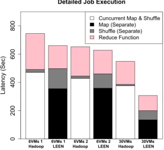
Detailed Job Execution Latency (Sec) 0 200 400 600 800
Cuncurrent Map & Shuffle Map (Separate) Shuffle (Separate) Reduce Function 6VMs 1 Hadoop 6VMs 1 LEEN 6VMs 2 Hadoop 6VMs 2 LEEN 30VMs Hadoop 30VMs LEEN
Fig. 8 Detailed performance of each stage in LEEN against native Hadoop for the three test sets
time of reduce tasks, and network latency which can affect the time to shuffle the intermediate data among the different data nodes.
For the test set (6VM 1), LEEN outperforms native Hadoop by 11.3%: Although the latency of the first two phases — map phase and shuffle phase — in native Hadoop is lower than LEEN (by only 9 seconds ), which can be explained due to the advantage of the concurrent execution of the map phase and the reduce phase (it is worth to note that it was expected that native Hadoop outperforms LEEN for the first two phases, especially that they transfer the same amount of data, but surprisingly the latency of these two phases were almost the same, which can be explained due to the map-skew [12] and the unfairness in the shuffled data between the nodes). However, the better fairness in reducers’ inputs data between nodes in LEEN results in balanced reduce functions executions, which in turn makes all reducers finish almost at the same time (the time taken by the best reduce function is 150 seconds and the time taken by the worst reduce function is 168 seconds). On the other hand, in native Hadoop, the skew reduce computation is very high and this results with longer execution time of the job: some nodes will be heavy loaded while other nodes are idles ( the time taken by the best reduce function is 33 seconds and the time taken by the worst reduce function is 231 seconds).
For the test set (6VM 2), LEEN speeds up native Hadoop by 4%: The latency of the first two phases — map phase and shuffle phase — in native
Hadoop is almost the same as in LEEN (less by only 14 seconds ), which can be explained due to higher locality in LEEN and thus the smaller transferred shuffled data. Similar to test set 1, the better fairness in reducers’ inputs data between nodes in LEEN results in balanced reduce functions executions and thus lower latency.
As we can see in Fig 8, the latency in native Hadoop in test set (6VMs 2) is lower that the one in test set (6VMs 1), although they both achieve almost the same locality. This can be explained due to the better fairness in data distribution of reducers’ inputs. On the other hand, the latency in LEEN in test set (6VMs 2) is lower that the one in test set (6VMs 1), although the fairness in data distribution of reducers’ inputs is better in test set (6VMs 1). This is due to the almost 40% reduction in data transfer that is achieved by LEEN in test set (6VMs 1).
For the test set (30VMs), LEEN outperforms native Hadoop by 45%: LEEN achieves a higher locality than in native Hadoop and thus a smaller transferred shuffled data than native Hadoop. LEEN also achieves better fair-ness in reducers’ inputs between nodes than in native Hadooop which in turn results in balanced reduce functions executions, all reducers therefore finish almost at the same time as shown in Fig 9-d (the time taken by the best reduce function is 40 seconds and the time taken by the worst reduce function is 55 seconds). On the other hand, in native Hadoop, skew reduce computation is very high as shown in Fig 9-c and this results with longer execution time of the job: some nodes will be heavy loaded while other nodes are idles ( the time taken by the best reduce function is 3 seconds and the time taken by the worst reduce function is 150 seconds).
5.5 Influence on load balancing
Finally in this subsection, we compare the system load balancing in LEEN against native Hadoop. As we stated earlier, LEEN is designed to mitigate the reduce computation skew through fair distribution of data among reducers: LEEN reduces the reduce computations variation by almost 85% compared to native Hadoop (from 90% to 13%). This results with balancing the load between reducers and lower latency in contrast to native Hadoop as shown in Fig 8-c and Fig 8-d.
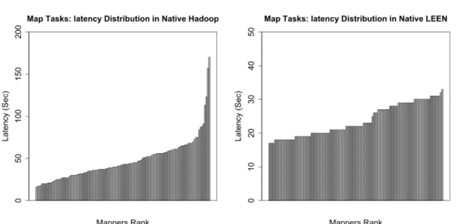
As shown in Fig 8-a, in native Hadoop, even though all map tasks receive the same amount of data, the slowest task takes more than 170 seconds while the fastest one completes in 16 seconds. However, in LEEN the executions of map tasks vary only by 19% as shown in 8-b: the slowest task takes more than 58 seconds while the fastest one completes in 40 seconds. This is because of the asynchronous map and reduce scheme: we start the shuffle phase after all maps are completed so here the complete I/O disk resources will be reserved to the map tasks, while in native Hadoop map tasks and reduce tasks will compete for the disk resources and this varies according the distribution of the keys during partitioning as well.
Map Tasks: latency Distribution in Native Hadoop Mappers Rank Latency (Sec) 0 50 100 150 200
(a) Running time of map tasks in native Hadoop
Map Tasks: latency Distribution in Native LEEN
Mappers Rank Latency (Sec) 0 10 20 30 40 50
(b) Running time of map tasks in LEEN
Reduce Functions: Latency Distribution in Hadoop
Reducers Rank Latency (Sec) 0 50 100 150
(c) Running time of reduce computations in native Hadoop
Reduce Functions: Latency Distribution in LEEN
Reducers Rank Latency (Sec) 0 10 20 30 40 50 60
(d) Running time of reduce computations in LEEN
Fig. 9 Load balancing: distrbution of the tasks run time for both map tasks and reduce comutation foe the test set 30VMs
It is important to mention that this load balancing in LEEN comes at the cost of fully resource utilization: the network resources are not used during map phase and the cpu usage is not utilized during the shuffle phase. We are going to investigate some techniques to overlap the map and the shuffle phase while preserving the same keys design in LEEN in the future.
6 Related Work
MapReduce has attracted much attention in the past few years. Some re-search has been dedicated to adopting MapReduce in different environments such as multi-core [6], graphics processors (GPU)s [5], and virtual machines
[26][27]. Many works on improving MapReduce performance has been intro-duced through locality-execution in the map phase [28][29], tuning the sched-ulers at OS-kernel [30]. Many case studies have demonstrated efficient usage of MapReduce for many applications including scientific applications [16][31] [32][33], machine learning applications [20][34] and graph analysis [35][36].
There have been few studies on minimizing the network congestion by data-aware reduction. Sangwon et al. have proposed pre-fetching and pre-shuffling schemes for shared MapReduce computation environments [37]. While the pre-fetching scheme exploits data locality by assigning the tasks to the nearest node to blocks, the pre-shuffling scheme significantly reduces the network overhead required to shuffle key-value pairs. Like LEEN, the pre-shuffling scheme tries to provide data-aware partitioning over the intermediate data, by looking over the input splits before the map phase begins and predicts the target reducer where the key-value pairs of the intermediate output are partitioned into a local node, thus, the expected data are assigned to a map task near the future reducer before the execution of the mapper. LEEN has a different approach: By separating the map and reduce phase and by completely scanning the keys’ frequencies table generating after map tasks, LEEN partitions the keys to achieve the best locality while guaranteeing near optimal balanced reducers’ inputs.Chen et al. have proposed Locality Aware Reduce Scheduling (LARS), which de-signed specifically to minimize the data transfer in their proposed grid-enabled MapReduce framework, called USSOP [38]. However, USSOP, due to the heterogeneity of grid nodes in terms of computation power, varies the data size of map tasks, thus, assigning map tasks associated with different data size to the workers according to their computation capacity. Obviously, this will cause a variation in the map outputs. Master node will defer the assignment of reduces to the grid nodes until all maps are done and then using LARS algorithm, that is, nodes with largest region size will be assigned reduces (all the intermediate data are hashed and stored as regions, one region may contain different keys). Thus, LARS avoids transferring large regions out. Despite that LEEN and LARS are targeting different environments, a key difference between LEEN and LARS is that LEEN provides nearly optimal locality on intermediate data along with balancing reducers’ computation in homogenous MapReduce systems.
Unfortunately, the current MapReduce implementations have overlooked the skew issue [15], which is a big challenge to achieve successful scale-up in a parallel query systems [39]. However, few studies have reported on the data skew impacts on MapReduce-based systems[13][40]. Qiu et al. have reported on the skew problems in some bioinformatics applications [13], and have discussed potential solutions towards the skew problems through implementing those applications using Cloud technologies. Lin analyzed the skewed running time of MapReduce tasks, maps and reduces, caused by the Zipfian distribution of the input and intermediate data, respectively [14].
Recent studies have proposed solutions to mitigate the skew problem MapRe-duce [41][42][43]. Gufler et al. have proposed to mitigate reMapRe-duce-skew by schedul-ing the keys to the reduce tasks based on cost model. Their solution uses
Top-Cluster to capture the data skew in MapReduce and accordingly identifies its most relevant subset for cost estimation. LEEN approaches the same prob-lem, which is computation skew among different reducers caused by the unfair distribution of reduces’ inputs, but LEEN also aims at reducing the network congestion by improving the locality of reducers’ inputs. Kwon et al. have pro-posed SkewReduce, to overcome the computation skew in MapReduce-based system where the running time of different partitions depends on the input size as well as the data values [42][44]. At the heart of SkewReduce, an optimizer is parameterized by user-defined cost function to determine how best to par-tition the input data to minimize computational skew. In later work, Kown et al. have proposed SkewTune [44]. SkewTune is a system that dynamically mit-igates skew which results from both: the uneven distribution of data and also uneven cost of data processing. LEEN approaches the same problem, which is computation skew among different reducers caused by the unfair distribution of reduces’ inputs, while assuming all values have the same size, and keeping in mind reduce the network congestion by improving the locality of reducers’ inputs. However, extending LEEN to the case when different values vary in size is ongoing work in our group.
7 Conclusions
Locality and fairness in data partitioning is an important performance fac-tor for MapReduce. In this paper, we have developed an algorithm named LEEN for locality-aware and fairness-aware key partitioning to save the net-work bandwidth dissipation during the shuffle phase of MapReduce caused by partitioning skew for some applications. LEEN is effective in improving the data locality of the MapReduce execution efficiency by the asynchronous map and reduce scheme, with a full control on the keys distribution among different data nodes. LEEN keeps track of the frequencies of buffered keys hosted by each data node. LEEN achieves both fair data distribution and performance under moderate and large keys’ frequencies variations. To quan-tify the data distribution and performance of LEEN, we conduct a compre-hensive performance evaluation study using Hadoop-0.21.0 with and without LEEN support. Our experimental results demonstrate that LEEN efficiently achieves higher locality, and balances data distribution after the shuffle phase. As a result,LEEN outperforms the native Hadoop by up to 45% in overall performance for different applications in the Cloud.
In considering future work, we are interested in adopting LEEN to the query optimization techniques [45][46] for query-level load balancing and fair-ness. As a long-term agenda, we are interested in providing a comprehensive study on the monetary cost of LEEN in contrast with Hadoop considering different pricing schemes (for example the as-you-go scheme and the pay-as-you-consume scheme[47]), knowing that LEEN always guarantees resource load balancing at the cost of concurrent resource access.
Acknowledgment
This work is supported by NSF of China under grant No.61232008, 61133008 and 61073024, the National 863 Hi-Tech Research and Development Pro-gram under grant 2013AA01A213, the Outstanding Youth Foundation of Hubei Province under Grant No.2011CDA086, the National Science & Tech-nology Pillar Program of China under grant No.2012BAH14F02, the Inter-disciplinary Strategic Competitive Fund of Nanyang Technological University 2011 No.M58020029, and the ANR MapReduce grant (ANR-10-SEGI-001). This work was done in the context of the H´em´era INRIA Large Wingspan-Project (see http://www.grid5000.fr/mediawiki/index.php/Hemera).
References
1. J. Dean, S. Ghemawat, Mapreduce: simplified data processing on large clusters, Commun. ACM 51 (2008) 107–113.
2. H. Jin, s. Ibrahim, T. Bell, L. Qi, H. Cao, S. Wu, X. Shi, Tools and technologies for building the clouds, Cloud computing: Principles Systems and Applications (2010) 3–20.
3. H. Jin, s. Ibrahim, L. Qi, H. Cao, S. Wu, X. Shi, The mapreduce pro-gramming model and implementations, Cloud computing: Principles and Paradigms (2011) 373–390.
4. M. Isard, M. Budiu, Y. Yu, A. Birrell, D. Fetterly, Dryad: distributed data-parallel programs from sequential building blocks, in: Proceedings of the 2nd ACM European Conference on Computer Systems (EuroSys ’07), Lisbon, Portugal, 2007, pp. 59–72.
5. B. He, W. Fang, Q. Luo, N. K. Govindaraju, T. Wang, Mars: a mapre-duce framework on graphics processors, in: Proceedings of the 17th inter-national conference on Parallel architectures and compilation techniques, Toronto, Ontario, Canada, 2008, pp. 260–269.
6. C. Ranger, R. Raghuraman, A. Penmetsa, G. Bradski, C. Kozyrakis, Eval-uating mapreduce for multi-core and multiprocessor systems, in: Proceed-ings of the 2007 IEEE 13th International Symposium on High Performance Computer Architecture (HPCA-13), Phoenix, Arizona, USA, 2007, pp. 13– 24.
7. Hadoop project, http://lucene.apache.org/hadoop (2011).
8. Yahoo!, yahoo! developer network, http://developer.yahoo.com/blogs/had oop/2008/02/yahoo-worldslargest-production-hadoop.html (2011).
9. Hadoop, applications powered by hadoop:,
http://wiki.apache.org/hadoop/PoweredB (2011).
10. S. Ghemawat, H. Gobioff, S.-T. Leung, The Google file system, SIGOPS - Operating Systems Review 37 (5) (2003) 29–43.
11. T. Condie, N. Conway, P. Alvaro, J. M. Hellerstein, K. Elmeleegy, R. Sears, Mapreduce online, in: Proceedings of the 7th USENIX Conference on
Net-worked Systems Design and Implementation (NSDI’10), San Jose, Califor-nia, 2010.
12. Y. Kwon, M. Balazinska, B. Howe, J. Rolia, A study of skew in mapreduce applications, http://nuage.cs.washington.edu/pubs/opencirrus2011.pdf. 13. X. Qiu, J. Ekanayake, S. Beason, T. Gunarathne, G. Fox, R. Barga,
D. Gannon, Cloud technologies for bioinformatics applications, in: Pro-ceedings of the 2nd Workshop on Many-Task Computing on Grids and Supercomputers (MTAGS ’09).
14. J. Lin, The curse of zipf and limits to parallelization: A look at the strag-glers problem in mapreduce, in: Proceedings of the 7th workshop on large-scale distributed systems for information retrieval (LSDS-IR’09).
15. D. J. DeWitt, M. Stonebraker, Mapreduce: A major step back-wards, 2008, http://databasecolumn.vertica.com/databaseinnovation/ma preduce-a-major-step-backwards.
16. K. Wiley, A. Connolly, J. P. Gardner, S. Krughof, M. Balazinska, B. Howe, Y. Kwon, Y. Bu, Astronomy in the cloud: Using MapReduce for image coaddition, CoRR abs/1010.1015.
17. R. Chen, M. Yang, X. Weng, B. Choi, B. He, X. Li,
Improving large graph processing on partitioned graphs in the cloud, in: Proceedings of the Third ACM Symposium on Cloud Comput-ing, SoCC ’12, ACM, New York, NY, USA, 2012, pp. 3:1–3:13. doi:10.1145/2391229.2391232.
URL http://doi.acm.org/10.1145/2391229.2391232
18. M. C. Schatz, Cloudburst: highly sensitive read mapping with mapreduce, Bioinformatics 25 (2009) 1363–1369.
19. A. Verma, X. Llor`a, D. E. Goldberg, R. H. Campbell, Scaling genetic algorithms using MapReduce, in: Proceedings of the 2009 9th International Conference on Intelligent Systems Design and Applications, 2009, pp. 13– 18.
20. A. Y. Ng, G. Bradski, C.-T. Chu, K. Olukotun, S. K. Kim, Y.-A. Lin, Y. Yu, MapReduce for machine learning on multicore, in: Proceedings of the twentieth Annual Conference on Neural Information Processing Sys-tems (NIPS’ 06), Vancouver, British Columbia, Canada, 2006, pp. 281– 288.
21. J. Lin, M. Schatz, Design patterns for efficient graph algorithms in mapre-duce, in: Proceedings of the Eighth Workshop on Mining and Learning with Graphs, Washington, USA, 2010, pp. 78–85.
22. Xen hypervisor homepage, http://www.xen.org/ (2011).
23. Amazon elastic compute cloud, http://aws.amazon.com/ec2/ (2011). 24. S. Ibrahim, H. Jin, L. Lu, S. Wu, B. He, L. Qi, Leen:
Locality/fairness-aware key partitioning for mapreduce in the cloud, in: Proceedings of the 2010 IEEE Second International Conference on Cloud Computing Technol-ogy and Science (CLOUDCOM’10), Indianapolis, USA, 2010, pp. 17–24. 25. R. Jain, D.-M. Chiu, W. Hawe, A quantitative measure of fairness and
discrimination for resource allocation in shared computer systems, DEC Research Report TR-301.
26. S. Ibrahim, H. Jin, L. Lu, L. Qi, S. Wu, X. Shi, Evaluating mapreduce on virtual machines: The hadoop case, in: Proceedings of the 1st International Conference on Cloud Computing (CLOUDCOM’09), Beijing, China, 2009, pp. 519–528.
27. S. Ibrahim, H. Jin, B. Cheng, H. Cao, S. Wu, L. Qi, Cloudlet: towards mapreduce implementation on virtual machines, in: Proceedings of the 18th ACM International Symposium on High Performance Distributed Computing (HPDC-18), Garching, Germany, 2009, pp. 65–66.
28. M. Zaharia, D. Borthakur, J. Sen Sarma, K. Elmeleegy, S. Shenker, I. Sto-ica, Delay scheduling: a simple technique for achieving locality and fairness in cluster scheduling, in: Proceedings of the 5th ACM European Confer-ence on Computer Systems (EuroSys’10), Paris, France, 2010, pp. 265–278. 29. S. Ibrahim, H. Jin, L. Lu, B. He, G. Antoniu, S. Wu, Maestro: Replica-aware map scheduling for mapreduce, in: Proceedings of the 12th IEEE/ACM International Symposium on Cluster, Cloud and Grid Com-puting (CCGrid 2012), Ottawa, Canada, 2012.
30. S. Ibrahim, H. Jin, L. Lu, B. He, S. Wu, Adaptive disk i/o scheduling for mapreduce in virtualized environment, in: Proceedings of the 2011 In-ternational Conference on Parallel Processing (ICPP’11), Taipei, Taiwan, 2011, pp. 335–344.
31. R. K. Menon, G. P. Bhat, M. C. Schatz, Rapid parallel genome indexing with MapReduce, in: Proceedings of the 2nd international workshop on MapReduce and its applications, San Jose, California, USA, 2011, pp. 51–58.
32. J. Ekanayake, S. Pallickara, G. Fox, Mapreduce for data intensive scientific analyses, in: Proceedings of the 2008 Fourth IEEE International Confer-ence on eSciConfer-ence, 2008, pp. 277–284.
33. T. Gunarathne, T.-L. Wu, J. Qiu, G. Fox, MapReduce in the Clouds for Science, in: Proceedings of the 2010 IEEE Second International Conference on Cloud Computing Technology and Science, 2010, pp. 565–572.
34. Y. Ganjisaffar, T. Debeauvais, S. Javanmardi, R. Caruana, C. V. Lopes, Distributed tuning of machine learning algorithms using MapReduce clus-ters, in: Proceedings of the 3rd Workshop on Large Scale Data Mining: Theory and Applications, San Diego, California, 2011, pp. 2:1–2:8. 35. S. Blanas, J. M. Patel, V. Ercegovac, J. Rao, E. J. Shekita, Y. Tian, A
comparison of join algorithms for log processing in mapreduce, in: Pro-ceedings of the 2010 international conference on Management of data, Indianapolis, Indiana, USA, 2010, pp. 975–986.
36. D. Logothetis, C. Trezzo, K. C. Webb, K. Yocum, In-situ mapreduce for log processing, in: Proceedings of the 2011 USENIX conference on USENIX annual technical conference, Portland, OR, 2011, pp. 9–9.
37. S. Seo, I. Jang, K. Woo, I. Kim, J.-S. Kim, S. Maeng, Hpmr: Prefetching and pre-shuffling in shared mapreduce computation environment, in: Pro-ceedings of the 2009 IEEE International Conference on Cluster Computing (CLUSTER’09), New Orleans, Louisiana, USA.
38. Y.-L. Su, P.-C. Chen, J.-B. Chang, C.-K. Shieh, Variable-sized map and locality-aware reduce on public-resource grids., Future Generation Comp. Syst. (2011) 843–849.
39. D. DeWitt, J. Gray, Parallel database systems: the future of high perfor-mance database systems, Commun. ACM 35 (1992) 85–98.
40. S. Chen, S. W. Schlosser, Map-reduce meets wider varieties of applications, Tech. Rep. IRP-TR-08-05, Technical Report, Intel Research Pittsburgh (2008).
41. G. Ananthanarayanan, S. Kandula, A. Greenberg, I. Stoica, Y. Lu, B. Saha, E. Harris, Reining in the outliers in map-reduce clusters us-ing mantri, in: Proceedus-ings of the 9th USENIX conference on Operatus-ing systems design and implementation (OSDI’10), Vancouver, BC, Canada, 2010, pp. 1–16.
42. Y. Kwon, M. Balazinska, B. Howe, J. Rolia, Skew-resistant parallel pro-cessing of feature-extracting scientific user-defined functions, in: Proceed-ings of the 1st ACM symposium on Cloud computing (SoCC ’10). 43. B. Gufler, N. Augsten, A. Reiser, A. Kemper, Load balancing in mapreduce
based on scalable cardinality estimates, in: Proceedings of the 2012 IEEE 28th International Conference on Data Engineering (ICDE ’12).
44. Y. Kwon, M. Balazinska, B. Howe, J. Rolia, Skewtune: mitigating skew in mapreduce applications, in: Proceedings of the 2012 ACM SIGMOD International Conference on Management of Data (SIGMOD ’12). 45. B. He, M. Yang, Z. Guo, R. Chen, W. Lin, B. Su, H. Wang, L. Zhou,
Wave computing in the cloud, in: Proceedings of the 12th conference on Hot topics in operating systems (HotOS’09).
46. B. He, M. Yang, Z. Guo, R. Chen, B. Su, W. Lin, L. Zhou, Comet: batched stream processing for data intensive distributed computing, in: Proceed-ings of the 1st ACM symposium on Cloud computing (SoCC ’10). 47. S. Ibrahim, B. He, H. Jin, Towards pay-as-you-consume cloud computing,
in: Proceedings of the 2011 IEEE International Conference on Services Computing (SCC’11), Washington, DC, USA, 2011, pp. 370–377.