HAL Id: hal-01298715
https://hal.archives-ouvertes.fr/hal-01298715v2
Submitted on 30 May 2016
HAL is a multi-disciplinary open access
archive for the deposit and dissemination of
sci-entific research documents, whether they are
pub-lished or not. The documents may come from
teaching and research institutions in France or
abroad, or from public or private research centers.
L’archive ouverte pluridisciplinaire HAL, est
destinée au dépôt et à la diffusion de documents
scientifiques de niveau recherche, publiés ou non,
émanant des établissements d’enseignement et de
recherche français ou étrangers, des laboratoires
publics ou privés.
Closed-form expressions of the exact Cramer-Rao,
bound for parameter estimation of BPSK, MSK, or
QPSK waveforms
Jean-Pierre Delmas
To cite this version:
Jean-Pierre Delmas. Closed-form expressions of the exact Cramer-Rao, bound for parameter
estima-tion of BPSK, MSK, or QPSK waveforms. IEEE Signal Processing Letters, Institute of Electrical and
Electronics Engineers, 2008, 15, pp.405 - 408. �10.1109/LSP.2008.921477�. �hal-01298715v2�
Closed-form expressions of the exact Cramer-Rao bound
for parameter estimation of BPSK, MSK or QPSK
waveforms
Jean-Pierre Delmas, Senior member, IEEE
Abstract
This paper addresses the stochastic Cramer-Rao bound (CRB) pertaining to the joint estimation of the carrier frequency offset, the carrier phase and the noise and signal powers of binary phase-shift keying (BPSK), minimum shift keying (MSK) and quaternary phase-shift keying (QPSK) modulated signals corrupted by additive white circular Gaussian noise. Because the associated models are gov-erned by simple Gaussian mixture distributions, an explicit expression of the Fisher information matrix is given and an explicit expression for the stochastic CRB of these four parameters are deduced. Spe-cialized expressions for low and high-SNR are presented as well. Finally, these expressions are related to the modified CRB and our proposed analytical expressions are numerically compared with the approximate expressions previously given in the literature.
Index terms: Stochastic Cramer Rao bound, Modified Cramer Rao bound, BPSK, MSK, QPSK.
EDICS Category: SAS-STAT,
Paper SPL-05038-2008.R1
D´epartement Communications, Image et Traitement de l’Information, Institut TELECOM SudParis, 9 rue Charles Fourier, 91011 Evry Cedex, FRANCE. Fax: +33-1-60 76 44 33, e-mail: [email protected]
1
Introduction
The stochastic Cramer-Rao bound (CRB) is a well known lower bound on the variance of any unbiased estimate, and as such, serves as useful benchmark for practical estimators. Unfortunately, the evaluation of this CRB is mathematically quite difficult when the observed signal contains, in addition to the parameters to be estimated, random discrete data and random noise. A typical example of such a situation that has been studied by many authors (see e.g., [1] and the references therein) is the observation of noisy linearly modulated waveforms that are a function of deterministic parameters such that the time delay, the carrier frequency offset, the carrier phase, noise and signal powers, as well as the data symbol sequence. Because the analytical computation of this CRB has been considered to be unfeasible, a modified CRB (MCRB) which is much simpler to evaluate than the exact CRB has been introduced in [2]. But this MCRB may not be as tight as the exact CRB [3] for joint estimation of all parameters. To circumvent this difficulty, asymptotic expressions at low [4] or high [5] signal-to-noise ratio (SNR) have been investigated. But unfortunately, these asymptotic expressions do not apply at moderate SNR, for which only combined analytical/numerical (see e.g., [5, 6, 1]) approaches are available until now.
In this paper, we investigate an analytical expression of the stochastic CRB (i.e., if the information symbols are viewed as nuisance parameters, and thus applicable in non data-aided estimation) associated with the joint estimation of the carrier frequency offset, the carrier phase and the noise and signal powers of BPSK, QPSK or MSK modulated signals corrupted by additive white circular Gaussian noise, which is valid for arbitrary SNR. This paper is organized as follows. After formulating the problem in Section 2, an explicit expression of the Fisher information matrix (FIM) associated with all the deterministic parameters is given in Section 3. Because the carrier frequency offset and the carrier phase parameters are decoupled from the signal noise and signal powers parameters, simple explicit expressions for the stochastic CRB of these four parameters are deduced. Specialized expressions for low and high-SNR are presented as well. Finally, in Section 4, our proposed analytical expressions are numerically compared with the previously given approximate expressions.
2
Problem formulation
Consider BPSK, QPSK or MSK modulated signals. The received signals are bandpass filtered and after down conversion the signal to baseband, the in-phase and quadrature components are paired to obtain complex signals. We assume Nyquist shaping and ideal sample timing so that the inter-symbol interference at each symbol spaced sampling instance can be ignored. In the presence of frequency offset and carrier phase, the signals at the output of the matched filters yield the observation vector y = (yk0, ..., yk0+K−1), with
yk= askei2πkνeiϕ+ nk,
for k = k0, ..., k0+ K− 1. {sk} is a sequence of independent identically distributed (IID) data symbols taking
values±1 and ±√2/2± i√2/2 with equal probabilities for BPSK and QPSK respectively and for MSK are defined by sk+1= iskck where ck is a sequence of independent BPSK symbols with equal probabilities where the original
value sk0 remains unspecified in the set {+1, +i, −1, −i}. The deterministic unknown parameters a, ν and ϕ
represent the amplitude, the carrier frequency offset normalized to the symbol rate and the carrier phase at k = 0. Finally, the sequence{nk} consists of IID zero-mean complex circular Gaussian noise random variables1of variance
σ2 def= E|n
k|2. The symbols sk are assumed to be independent from nk. If no a priori information is available
concerning the transmitted symbols, the distribution of y is parameterized by θ def= (ν, ϕ, a, σ). We note that the MSK is modelled equivalently (see e.g., [7]) by sk = ik−k0bksk0 where bkis another sequence of independent BPSK
symbols{−1, +1} with equal probabilities. Consequently, similar to the BPSK and QPSK, (yk)k=k0,...,k0+K−1 are
independently non-identically distributed along the following mixture of circular Gaussian distribution2:
p(yk; θ) = 1 Lπσ2 L ∑ l=1 exp ( −|yk− asl,kei2πkνeiϕ|2 σ2 ) , (2.1) with sl,k=±1 (L = 2), sl,k=± √
2/2± i√2/2 (L = 4) or sl,k= ik−k0blsk0 with bl=±1 (L = 2) associated with
BPSK, QPSK or MSK, respectively.
3
Stochastic CRB: analytical results
3.1
General closed-form expression
Using the independence of the random variables yk, the Fisher information matrix (FIM) is given (elementwise)
by: (IF)i,j=− k0+K∑−1 k=k0 E ( ∂2ln p(y k; θ) ∂θi∂θj ) i, j = 1, . . . , 4, (3.2)
where the PDF’s (2.1) take the following forms:
p(yk; θ) = 1 πσ2 exp ( −|yk|2+ a2 σ2 ) c(yk),3
where c(yk) is respectively equal to cosh
(a σ2 g1(yk) ) , cosh ( a σ2√2 g1(yk) ) cosh ( a σ2√2 g2(yk) ) and cosh(σa2 g3(yk) )
for the BPSK, QPSK and MSK respectively, with g1(yk)
def
= 2ℜ(ei2πkνeiϕy∗
k), g2(yk)
def
= 2ℑ(ei2πkνeiϕy∗ k) and
g3(yk)
def
= 2ℜ(ik−k0ei2πkνeiϕs
k0yk∗). Extending the approach used in [8] for the parameters a and σ only and in [9]
for the direction of arrival (DOA) parameters, the following lemma is proved in Appendix A:
Lemma 1 The parameter θ = (ν, ϕ, a, σ) is partitioned in two decoupled parameters (ν, ϕ) and (a, σ) in the FIM
associated with the BPSK, QPSK and MSK:
IBPSK= IMSK= [ I(1)B O O I(2)B ] , IQPSK= [ I(1)Q O O I(2)Q ] 1
Note that many papers consider the parameters a2and σ2denoted usually as the symbol energy Esand the noise power
spectral density N0 as known. They usually suppose a unit variance for the noise and use the ratio ϵ def
= (Es/N0)1/2as the modulation amplitude, but in practice these two parameters are unknown as well.
2Usually for such a mixture, explicit closed-form expressions of the CRB are not available. 3
with I(1)B = 2ρ2(1− f1(ρ)) [ (2π)2∑k0+K−1 k=k0 k 2 2π∑k0+K−1 k=k0 k 2π∑k0+K−1 k=k0 k K ] I(2)B = 2K ρ a2 [ 1− f2(ρ) 2√ρf2(ρ) 2√ρf2(ρ) 2(1− 2ρf2(ρ)) ] I(1)Q = 2ρ2(1− (1 + ρ)f1( ρ 2)) [ (2π)2∑k0+K−1 k=k0 k 2 2π∑k0+K−1 k=k0 k 2π∑kk=k0+K−1 0 k K ] I(2)Q = 2K ρ a2 [ 1− f2(ρ2) 2√ρf2(ρ2) 2√ρf2(ρ2) 2(1− 2ρf2(ρ2)) ]
where ρ is the SNR aσ22 and f1 and f2 are the following decreasing functions of ρ:
f1(ρ) def = 2e −ρ √ 2π ∫ +∞ 0 e−u22 cosh(u√2ρ)du, f2(ρ) def = 2e −ρ √ 2π ∫ +∞ 0 u2e−u22 cosh(u√2ρ)du.
The determinants of I(1)B and I(1)Q do not depend on the time k0at which the first sample is taken and consequently
the CRB for the frequency does not depend on it either, but the CRB for the phase does. The minimum value for this CRB is attained for k0=−(K − 1)/2. This particular choice of k0 renders I
(1) B and I
(1)
Q diagonal and we
obtain in this case the following result, where the MCRB are straightforwardly derived from [2]: MCRB(θi) = 1 Ey,s ( ∂2ln p(y/s;θ) ∂θ2 i ), i = 1, . . . , 4.
Result 1 The CRB for the joint estimation of the parameters (ν, ϕ, a, σ) associated with the BPSK and MSK are
given by: CRB(ν) = 6 (2π)2K(K2− 1)ρ(1 − f 1(ρ)) = MCRB(ν) ( 1 1− f1(ρ) ) (3.3) CRB(ϕ) = 1 2Kρ(1− f1(ρ)) = MCRB(ϕ) ( 1 1− f1(ρ) ) (3.4) CRB(a) = a 2(1− 2ρf 2(ρ)) 2Kρ(1− f2(ρ)− 2ρf2(ρ)) = MCRB(a) ( 1− 2ρf2(ρ) 1− f2(ρ)− 2ρf2(ρ) ) (3.5) CRB(σ) = a 2(1− f 2(ρ)) 4Kρ(1− f2(ρ)− 2ρf2(ρ)) = MCRB(σ) ( 1− 2ρf2(ρ) 1− f2(ρ)− 2ρf2(ρ) ) . (3.6)
The CRBs associated with the QPSK are obtained by replacing f1(ρ) and f2(ρ) by, respectively, (1 + ρ)f1(ρ2) and
f2(ρ2) in (3.3), (3.4), (3.5) and (3.6).
Note that the proof of the decoupling that is not trivial (see (5.11),(5.12)) has not appeared in the literature despite the first expressions CRB(ν) and CRB(ϕ) coincide with the expressions given in [10] for CRB(ν) with (ϕ, a, σ) known and CRB(ϕ) with (ν, a, σ) known, for the BPSK only. The first expressions CRB(ν) and CRB(ϕ) does not appear in [10] for MSK and QPSK including for (ϕ, a, σ) or (ν, a, σ) known. Using the definition of f1
and f2, these asymptotic CRBs coincide with the MCRB for high SNR. This extends a property proved in [3] for
a scalar parameter only.
3.2
Low-SNR expression
For low SNR, f1(ρ) and f2(ρ) approach 1. We resort to a Taylor series expansion of these functions obtained
by expanding e−ρ and cosh(u√2ρ) around ρ = 0. Then, using the values (2n)!/2nn! of the moments of order
2n of zero-mean unit variance Gaussian random variables, we obtain after tedious, but straightforward algebraic manipulations: f1(ρ) = 1− 2ρ + 4ρ2− 40 3 ρ 3+208 3 ρ 4+ o(ρ4), f2(ρ) = 1− 4ρ + 16ρ2− 256 3 ρ 3+12544 21 ρ 4+ o(ρ4).
Inserting these expansions in Result 1 allows us to prove the following result4:
Result 2 The CRB for the joint estimation of the parameters (ν, ϕ, a, σ) associated with the BPSK, MSK and
QPSK are given for low SNR by:
CRB(ν) = 6 (2π)2K(K2− 1) L! L2ρL(1 + Lρ + o(ρ)) = MCRB(ν) L! L2ρL−1(1 + Lρ + o(ρ)) (3.7) CRB(ϕ) = 1 2K L! L2ρL(1 + Lρ + o(ρ)) = MCRB(ϕ) L! L2ρL−1(1 + Lρ + o(ρ)) (3.8) CRB(a) = a 2 KαLρL (1 + Lρ + o(ρ)) = MCRB(a) 2 αLρL−1 (1 + Lρ + o(ρ)) (3.9) CRB(σ) = a 2 KβLρL−1 (1 + γLρ3−L/2+ o(ρ3−L/2)) = MCRB(σ) 4 βLρL−2 (1 + γLρ3−L/2+ o(ρ3−L/2)), (3.10)
with L = 2 for BPSK and MSK and L = 4 for QPSK, and α2 = 4, α4= 16/3, β2 = 2, β4 = 16/3, γ2 =−16/3
and γ4= 4.
We note that (3.7) and (3.8) for BPSK and QPSK are refinements of the expressions of CRB(ν) and CRB(ϕ) given in [4].
3.3
High-SNR expression
For high SNR, the MCRB approaches the CRB at the same rate that f1(ρ) and f2(ρ) approach 0. Because we
prove in Appendix B that these functions are bounded above by √e−ρπρ and more precisely that f1(ρ)/e
−ρln(2)
√πρ tends to 1 when ρ tends to ∞, the CRB are practically equal to the MCRB for moderate SNR. For example: ρ = 2 (3dB), and ρ = 4 (6dB)] give respectively the upper bound 0.05 and 0.005 for f1(ρ) and f2(ρ), and consequently
the ratios CRB/MCRB is around one from these values of SNR.
4
Numerical results
The analytical result 1 is numerically compared with the approximations given in result 2 and to the approximations given in [4] for CRB(ν) and CRB(ϕ) of BPSK and QPSK at low SNR.
In these conditions, we see good agreement between the numerical values derived from results 1 and 2 in a large range of low SNR. Furthermore, we note that the ratio CRB/MCRB is unbounded except for the noise power of BPSK and MSK for which it tends to 2 when the SNR tends to 0.
4Of course these bounds are going to infinity as the SNR decreases to zero, consequently for the parameters ν and ϕ with finite support, these results are useful for not too low-SNR only (typically in the range [-5dB, 0dB]).
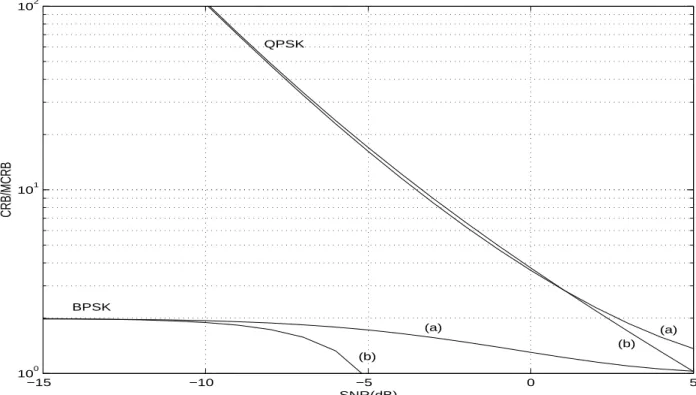
−15 −10 −5 0 5 100 101 102 103 SNR(dB) CRB/MCRB BPSK QPSK (a) (b) (c) (a) (b) (c)
Fig. 1 Ratio CRB(ν)/MCRB(ν)=CRB(ϕ)/MCRB(ϕ) at low SNR: (a) exact value given by (3.3), (3.4), (b) approximate value given by (3.7), (3.8), (c) approximate value given in [4].
−15 −10 −5 0 5 100 101 102 103 SNR(dB) CRB/MCRB BPSK QPSK (a) (b) (a) (b)
−15 −10 −5 0 5 100 101 102 SNR(dB) CRB/MCRB BPSK QPSK (a) (b) (a) (b)
Fig. 3 Ratio CRB(σ)/MCRB(σ) at low SNR: (a) exact value given by (3.6), (b) approximate value given by (3.10).
5
Appendix: Proof of Lemma 1
To evaluate the FIM (3.2) for the BPSK, the partial derivatives are straightforwardly derived, in particular:
∂2ln p(y k; θ) ∂ϕ2 = a2g2 2(yk) σ4 1 cosh2 ( ag1(yk) σ2 ) −ag1(yk) σ2 tanh ( ag1(yk) σ2 ) ∂2ln p(yk; θ) ∂a∂ϕ = − ag1(yk)g2(yk) σ4 1 cosh2 ( ag1(yk) σ2 ) −g2(yk) σ2 tanh ( ag1(yk) σ2 ) (5.11) ∂2ln p(y k; θ) ∂a∂ν = (2πk) ∂2ln p(y k; θ) ∂a∂ϕ ∂2ln p(y k; θ) ∂σ∂ϕ = 2a2g 1(yk)g2(yk) σ5 1 cosh2 ( ag1(yk) σ2 ) +2ag2(yk) σ3 tanh ( ag1(yk) σ2 ) (5.12) ∂2ln p(y k; θ) ∂σ∂ν = (2πk) ∂2ln p(y k; θ) ∂σ∂ϕ .
Using the regularity condition ∂ ∂θi
∫
p(yk; θ)dyk =
∫ ∂p(yk;θ)
∂θi dyk which is fulfilled for finite mixtures of Gaussian
distributions, the following property holds: E ( ∂ln p(yk;θ) ∂a ) = 0. With ∂ln p(yk;θ) ∂a =− 2a σ2+ g1(yk) σ2 tanh ( ag1(yk) σ2 ) , we obtain E ( g1(yk)tanh ( ag1(yk) σ2 )) = 2a.
This identity enables us to straightforwardly derive the terms of I(2)B using the definition of the function f2(ρ) =
E ( g12(yk) 2σ2 1 cosh2(ag1(yk) σ2 ) )
, where the random variable g1(yk) is equally weighted mixed Gaussian (N (−2a; 2σ2) and
N (+2a; 2σ2)).
To evaluate I(1)B , we note that g1(yk) = 2ask +
(
ei2πkνeiϕn∗k+ e−i2πkνe−iϕnk
)
and g2(yk) =
−i(ei2πkνeiϕn∗
k− e−i2πkνe−iϕnk
)
. Because sk and nk are independent and the two Gaussian random variables
ei2πkνeiϕn∗
three random variables sk, ei2πkνeiϕn∗k+ e−i2πkνe−iϕnk and ei2πkνeiϕn∗k− e−i2πkνe−iϕnk are collectively
indepen-dent and thus g1(yk) and g2(yk) are independent. Using the definition of the function f1(ρ) = E
( 1 cosh2(ag1(yk) σ2 ) ) , the terms of I(1)B are derived.
Because g1(yk) and g2(yk) are independent and zero mean, E(∂
2ln p(y k;θ) ∂a∂ϕ ) = E( ∂2ln p(yk;θ) ∂σ∂ϕ ) = E( ∂2ln p(yk;θ) ∂a∂ν ) = E(∂2ln p(yk;θ)
∂σ∂ν ) = 0. This implies that the parameters (ν, ϕ) and (a, σ) are decoupled in the FIM.
For the MSK, the derivations follow the same lines, replacing g1(yk) by g3(yk).
Finally for the QPSK, evaluating the partial derivatives ∂2ln p(yk;θ)
∂θi∂θj and taking their expectation are derived
in the same way, provided the log-likelihoods associated with g1(yk) and g2(yk) are gathered, and the hypothesis
of independence ofℜ(sk) andℑ(sk) is taken into account.
6
Appendix: Bounds on f
1(ρ) and f
2(ρ)
For high SNR, using the inequality cosh(u1√
2ρ) < 2e−u
√2ρ
, we obtain after simple algebraic manipulations:
f1(ρ) < 4Q( √ 2ρ) and f2(ρ) < 4 ( (2ρ + 1))Q(√2ρ)− √ 2ρ √ 2πe −ρ), (6.13)
where Q(x) is the error function ∫x+∞√1
2πe
−u2
2 du classically bounded above by 1
x√2πe
−x2
2 . Applying this upper
bounds in (6.13) gives: f1(ρ) < e
−ρ
√πρ and f2(ρ) < e
−ρ
√πρ. To specify the upper bound of f1(ρ), we use the following
expansion 1 cosh(u√2ρ) = 2e −u√2ρ(1 + e−u√2ρ)−1= 2 +∞ ∑ k=0 (−1)ke−(k+1)u√2ρ.
Inserting this into f1(ρ), we obtain after simple algebraic manipulations the following alternating expansion:
f1(ρ) = 4 +∞
∑
k=0
(−1)keρ[(k+1)2−1]Q[(k + 1)√2ρ]. (6.14)
Using the standard bounds 1
x√2π(1− 1 x2)e− x2 2 ≤ Q(x) ≤ 1 x√2πe −x2 2 and ln(2) = −∑∞ k=1 (−1)k k in (6.14) proves
after simple algebraic manipulations that f1(ρ)/
e−ρln(2)
√πρ tends to 1 when ρ tends to∞.
References
[1] N. Noels, H. Steendam and M. Moeneclaey, “The true Cramer-Rao bound for carrier frequency estimation from a PSK signal,” IEEE Trans. Commun., vol. 52, no. 5, pp. 834-844, May 2004.
[2] A.N.D. Andrea, U. Mengali and R. Reggiannini, “The modified Cramer-Rao bound and its application to synchronization problems,” IEEE Trans. Commun., vol. 42, no. 2/3/4, pp. 1391-1399, Feb.-Apr. 1994.
[3] M. Moeneclaey, “On the true and modified Cramer-Rao bound for the estimation of a scalar parameter in the presence of nuisance parameters,” IEEE Trans. Commun., vol. 46, no. 11, pp. 1536-1544, November 1998. [4] H. Steendam, M. Moeneclaey, “Low SNR limit of the Cramer-Rao bound for estimating the carrier phase and
frequency of a PAM, PSK or QAM waveform,” IEEE Commun. letters, vol. 5, no. 5, pp. 218-220, May 2001. [5] G.N. Tavares, L.M. Tavares and M.S. Piedade, “Improved Cramer-Rao bounds for phase and frequency
esti-mation with M -PSK signals,” IEEE Trans. Commun., vol. 49, no. 12, pp. 2083-2087, December 2001.
[6] F. Rice, B. Cowley, B. Moran and M. Rice, “Cramer-Rao bounds for the QAM phase and frequency estimation,”
IEEE Trans. Commun., vol. 49, no. 9, pp. 1582-1591, September 2001.
[7] J. Lebrun and P. Comon, “An algebraic approach to blind identification of communication channel,” in Int.
[8] N. S. Alagha, “Cramer-Rao bounds for SNR estimates for BPSK and QPSK modulated signals,” IEEE
Com-mun. letters, vol. 5, no. 1, pp. 10-12, January 2001.
[9] J.P. Delmas, H. Abeida, “Cramer-Rao bounds of DOA estimates for BPSK and QPSK modulated signals,”
IEEE Trans. on Signal Processing, vol. 54, no. 1, pp. 117-126, January 2006.
[10] W.C. Cowley, “Phase and frequency estimation for PSK packets: Bounds and algorithms,” IEEE Trans.
![Fig. 1 Ratio CRB(ν)/MCRB(ν)=CRB(ϕ)/MCRB(ϕ) at low SNR: (a) exact value given by (3.3), (3.4), (b) approximate value given by (3.7), (3.8), (c) approximate value given in [4].](https://thumb-eu.123doks.com/thumbv2/123doknet/11352629.284832/6.892.100.795.127.522/ratio-mcrb-mcrb-exact-value-given-approximate-approximate.webp)