Multiscale proper generalized decomposition based on the partition of unity
Texte intégral
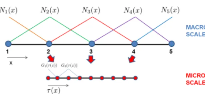
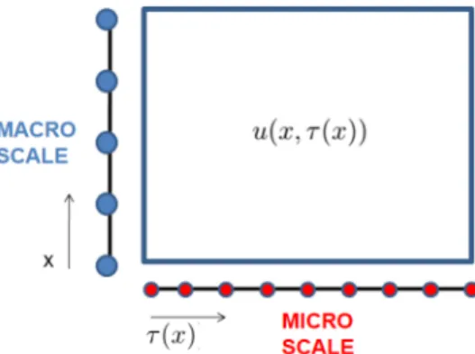
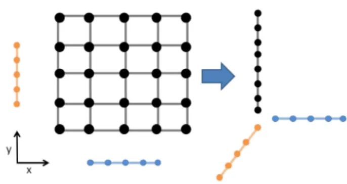
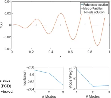
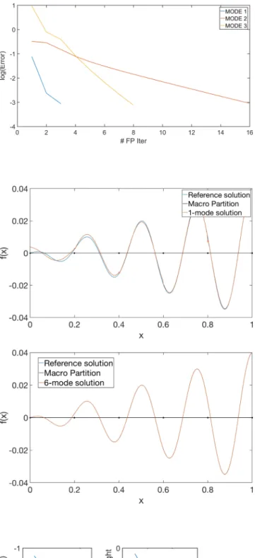
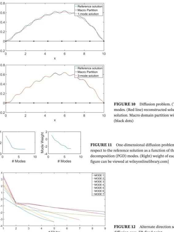
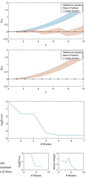
Figure

Documents relatifs
Pourquoi en physique classique existe-t-il deux types de forces : des forces « normales » et des forces d’inertie (parfois appelées pseudo forces) qui interviennent dans les
On commencera dans un premier temps par rappeler les notions de base du mouvement brownien standard mB et le mouvement brownien fractionnaire mBf, puis, nous ´etablirons
questions ou objets d’études sont absents des sciences de l’éducation : les finalités éducatives, la valeur de formation des contenus sous la forme de ce que le monde
1) L’achat au profit de ses adhérents des matières premières et des intrants nécessaires à l’agriculture et à la pêche. 2) La conservation, la transformation, le stockage,
When service level interworking is needed, in the case of an instant message being transmitted from LTE to GSM, the IP-SM-GW must translate the SIP headers in accordance
Figure 106 : Synoptique d’un étage d’amplification à Transistor 119 Figure 107 : Influence des pertes sur les impédances ramenées dans le circuit de sortie 120 Figure 108
Mais dans les années 1990, des chercheurs japonais ont mis en évidence un état ferromagnétique non- conventionnel dans le GaAs dopé avec une faible concentration de Mn (environ 5
