Science Arts & Métiers (SAM)
is an open access repository that collects the work of Arts et Métiers Institute of Technology researchers and makes it freely available over the web where possible.
This is an author-deposited version published in: https://sam.ensam.eu Handle ID: .http://hdl.handle.net/10985/19155
To cite this version :
Mohamed BEN BETTAIEB, Farid ABED-MERAIM - Formability prediction of substrate-supported metal layers using a non-associated plastic flow rule - Journal of Materials Processing Technology - Vol. 287, p.116694 - 2021
Any correspondence concerning this service should be sent to the repository Administrator : [email protected]
-1-
Formability prediction of substrate-supported metal layers
using a non-associated plastic flow rule
Mohamed Ben Bettaieb, Farid Abed-Meraim
Université de Lorraine, CNRS, Arts et Metiers Institute of Technology, LEM3, F-57070 Metz, France DAMAS, Laboratory of Excellence on Design of Alloy Metals for low-mAss Structures, Université de Lorraine, France
Abstract
When manufacturing flexible devices, it is quite common that localized necking appears due to the low ductility of the metal sheets used. To delay the inception of such localized necking, several industrial companies have proposed a promising technical solution based on the bonding of elastomer substrates to the metal sheets used in the manufacturing processes. In this context, the comprehensive numerical understanding of the impact of such substrate coating on the improvement of the ductility of elastomer-supported metal layers still remains a challenging goal. To achieve this goal, the bifurcation approach as well as the Marciniak and Kuczynski model are used to predict the occurrence of localized necking. The mechanical behavior of the metal layer is modeled by a non-associated anisotropic plasticity model. The adoption of non-associated plastic flow rule allows separating the description of the plastic potential from that of the yield function, which is essential to accurately model strong plastic anisotropy characterizing cold-rolled sheets. As to the elastomer substrate, its mechanical behavior is described by a neo-Hookean law. The paper presents a variety of numerical results relating to the prediction of plastic strain localization in both freestanding and elastomer-coated metal layers. The effects of the non-associativity of the plastic flow rule for the metal layer and the addition of an elastomer substrate on the predictions of localized necking are especially underlined. It is shown that the ductility limits predicted by the non-associated elasto-plastic model are lower than their counterparts determined by an associated plasticity model. It is also proven that adhering an elastomer layer to the metal layer can substantially delay the initiation of plastic strain localization.
-2-
Keywords: Formability prediction. Substrate-supported metals. Non-associated plasticity.
Bifurcation and imperfection approaches.
1. Introduction
Sheet metal forming operations are usually restricted by the initiation of plastic strain localization because of the low ductility of the utilized sheets. This kind of plastic instability marks the ultimate deformation that formed sheet metals can sustain, since localized necking is usually closely followed by material failure. To enhance the ductility of metallic parts and components, several industrial actors have developed a technological solution based on perfectly joining elastomer substrates to the original freestanding metal sheets. This solution proved to be effective, as it substantially improves ductility as discussed by Alaca et al. (2002) and increases energy absorption as revealed by Xue and Hutchinson (2007). The ductility characteristics of metal/polymer line structures formed by depositing Au/Cr lines on a semiflexible polyimide substrate, pyromellitic dianhydride-oxydianiline (PMDA-ODA), have been experimentally investigated by Chiu et al. (1994) using a stretch deformation technique. The role of strain hardening for the deformation of thin Cu films has been quantitatively investigated by Hommel and Kraft (2001) by conducting specialized tensile testing allowing the simultaneous characterization of the film stress and the dislocation density as a function of plastic strain. More recently, Alaca et al. (2002) have studied the failure by debonding of 400 nm Al thin films on 152 µm-thick polyimide substrates in uniaxial tension experiments and have demonstrated the effect of substrate layer on the delay of failure in this case. Due to its effectiveness, this strategy has been widely used to design a number of flexible electronic devices, such as stretchable interconnects for elastic electronic surfaces (Lacour et al., 2005), multifunctional capacitive sensors for stretchable electronic skins (Cotton et al., 2009), chromium thin films bonded to polymer substrates (Cordill et al., 2010), and elastically stretchable metal conductors (Graudejus et al., 2012). However, necking instabilities in substrate-supported metal layers under arbitrary biaxial loading states remain poorly analyzed and understood from the experimental point of view. Indeed, the most commonly conducted experiments for such metal/substrate bilayers are uniaxial tensile tests. Furthermore, structural instabilities (due to the wrinkling of the elastomer layer and the interfacial delamination between the two layers) cannot be avoided during biaxial loading experiments. These phenomena have a significant influence on the ductility limit of the bilayer. Hence, quantitative correlation between the necking limit strain and both the material
-3-
properties and geometric characteristics of the bilayer is difficult to be clearly established from experimental investigations, as it remains challenging to discriminate the effects of material and structural instabilities on the ductility limit of the bilayer. To address this issue, several theoretical and numerical approaches have been developed in the literature to accurately establish the correlation between the mechanical and geometric properties of both layers and the ductility limit of the bilayer. Note that the formability limit for substrate-supported metal layers has been first numerically predicted by Jia and Li (2013) using the concept of forming limit diagrams (FLDs). In the latter investigation, the mechanical behavior of the metal and elastomer layers has been modeled, respectively, by the rate-independent deformation theory of plasticity and a neo-Hookean model, while the ductility limit has been predicted by the Rice bifurcation approach (Rice, 1976). The impact of fixing an elastomer substrate on the enhancement of the predicted limit strains has been clearly shown in Jia and Li (2013). The developments of Jia and Li (2013) have been enlarged in Ben Bettaieb and
Abed-Meraim (2015) by extending the study to two new frameworks: (i) an associated flow
theory of plasticity, as an alternative for modeling the mechanical behavior of the metal layer, and (ii) the initial imperfection approach of Marciniak and Kuczynski (1967), as an additional criterion to predict plastic strain localization. The positive effect of the elastomer substrate on the ductility of the bilayer, initially highlighted in Jia and Li (2013), has been confirmed in
Ben Bettaieb and Abed-Meraim (2015) for both constitutive theories. Subsequently, the influence of the mechanical behavior of the metal layer on the ductility of the bilayer has been thoroughly studied in several contributions. For instance, the effects of kinematic hardening or strain rate sensitivity on the occurrence of localized necking in substrate-supported metal layers have been analyzed in Ben Bettaieb and Abed-Meraim (2017a, b), respectively. In the previous investigations, the mechanical behavior of the metal layer has been restricted to isotropic plasticity. However, it is well recognized that the mechanical behavior of metal sheets is highly anisotropic. It has been revealed in several contributions, based on phenomenological approaches (Barlat, 1987) or multiscale analyses (Akpama et al., 2017), that such plastic anisotropy has a substantial impact on the occurrence of localized necking, especially for strain paths near equibiaxial tension state. In the earlier scientific literature, several plastic yield functions have been set up to describe plastic anisotropy. The majority of anisotropic yield functions are based on the Associated Flow Rule (AFR), which assumes that the yield function and the plastic potential are the same. Following the AFR concept, various yield functions have been developed in the literature such as: Hill (Hill, 1948), Karafillis and Boyce (Karafillis and Boyce, 1993), Barlat (Barlat et al., 2003), Bron and Besson (Bron and
-4-
Besson, 2004), Banabic (Banabic et al., 2005) yield functions. In the last decades, several attempts have been dedicated to improving the modeling of initial plastic anisotropy and its evolution by developing more advanced constitutive frameworks. As a consequence, non-associated flow rule (NAFR) models have been suggested as alternatives to classical AFR models. The NAFR concept relies on the idea of dissociation between the plastic potential and the yield criterion. This dissociation allows overcoming the limitations of the classical AFR models, and thus to ensure more accurate modeling of the plastic flow. One of the most important benefits of using NAFR models, instead of classical AFR ones, is the extra freedom afforded by considering separate plastic potential and yield locus. Such a separation allows reproducing elaborate material behavior using simple mathematical formulations, as suggested by Yoon et al. (2007), or by the combination of two different functions, as proposed by Paulino and Yoon (2015) who have combined the Hill and the Yld2000-2d (Barlat et al., 2003) functions and Stoughton (2002) who has proposed a non-associated flow rule in which the plastic potential (resp. the yield surface) is defined by the Hill criterion based on the measured r-values (resp. yield stresses). The interest in adopting NAFR models, compared to the classical AFR ones, in the modeling of some forming processes has been highlighted by several authors. In this field, Yoon et al. (2000) have used a NAFR models, based on an asymmetric nonquadratic yield function, to predict the cup profile during the drawing of a circular blank. This later investigation has been extended by Yoon et al. (2010)
to predict earing profiles for strongly textured aluminum sheets. More recently, Paulino and
Yoon (2015) have used a NAFR model to accurately model the mechanical behavior during
cup drawing process. In the current investigation, a NAFR framework is used to model the metal layer mechanical behavior, where both the yield function and plastic potential are modeled by the Yld2000-2d anisotropic criterion. The parameters adopted for the yield function are fitted using the directional yield stresses for uniaxial loading corresponding to every 15° from rolling to transverse direction (, , , , , , ) in addition to the equibiaxial yield stress (b). As to the parameters adopted for the plastic potential function, they are optimized by using r-values for uniaxial tension tests in different orientations (r , 0 r , 15 r , 30 r , 45 r , 60 r , 75 r ) as well as for equibiaxial loading (90 r ). The use of b
the non-associated version of the Yld2000-2d anisotropic model is motivated by its high flexibility and the availability of the corresponding anisotropy parameters in the literature. In this field, one can quote Safaei et al. (2014a, b) who have identified the anisotropy parameters of a NAFR, based on the Yld2000-2d model, for the 2090-T3 aluminum alloy. More recently,
-5-
Hippke et al. (2017) have identified the anisotropy parameters for AA5042 and AA6016 aluminum alloys.As to the elastomer layer, its mechanical behavior is modeled by the well-known neo-Hookean law. The resulting mechanical model for the substrate-supported metal layer is coupled with the bifurcation theory and the imperfection approach of Marciniak and Kuczynski to predict the ductility limit of the bilayer. The application of these necking criteria requires the integration of the constitutive model and the determination of the relevant tangent modulus for each layer. To this end, an implicit integration scheme is established to solve the constitutive equations of the NAFR model (Safaei et al., 2015). It should be noted that very few works in the literature have used the associated version of the Yld2000-2d anisotropic criterion in conjunction with the imperfection approach of Marciniak and Kuczynski to predict the ductility limit. In this area, one can cite Butuc et al. (2011) who have used the Yld2000-2d criterion to predict the formability limit in DC06 steel sheets or Ozturk et al. (2014) who have applied this anisotropic function to predict the ductility limit in DP600 advanced high strength steel sheets. However, it is the first time that the non-associated version is coupled with the above-mentioned localized necking criterion. Hence, the effect of the non-associativity of the flow rule on the predicted ductility limits for both the freestanding metal layer and the bilayer will be specifically analyzed. Also, the beneficial impact of the elastomer substrate coating on the ductility of bilayer components is once again confirmed in the current investigation.
The layout of the remaining part of the paper is as follows:
• Section 2 is dedicated to the presentation of the constitutive frameworks selected to model the behavior of the elastomer and metal layers, as well as the adopted necking criteria.
• Section 3 presents the numerical algorithms established for the FLD predictions based on both localized necking criteria.
• A variety of numerical predictions and results are provided in Section 4, where the impact of both the anisotropy parameters and the addition of an elastomer layer on the ductility limit is extensively discussed and commented.
-6-
Notations, conventions and abbreviations
The derivations presented in this paper are carried out using classic conventions. Note that the assorted notations can be combined. Additional notations will be clarified as needed, following related equations.
2. Theoretical modeling
2.1. Necking criteria
2.1.1. Loading and boundary conditions
To predict the onset of strain localization, biaxial loading is applied to the metal/elastomer bilayer, where the strain rate components 11, 22 and 12 are set to 1, and 0, respectively.
The strain-path ratio is taken to range between 1 2 / and 1. Both layers are assumed to be
Vectorial and tensorial fields are designated by bold letters and symbols Scalar variables and parameters are represented by thin letters and symbols
time derivative of 1 inverse of tensor T transpose of tensor
tensor product of two vectors
tensor product of two second-order tensors simple contraction or contraction on one index double contraction or contraction on two indices
Euclidian norm of E
quantity associated with the elastomer layer M
quantity associated with the metal layer B
quantity associated with behavior in the band S
quantity associated with behavior in the safe zone
ˆ
the in-plane counterpart of , equal to 1
2 if is a vector and to 11 12 21 22 if is a second-order tensor, etc…
I2 second-order identity tensor
AFR associated flow rule NAFR non-associated flow rule
-7-
very thin (Fig. 1). Furthermore, they are assumed to remain perfectly bonded during the loading. As a consequence, the in-plane components of the deformation gradient fM
within the metal layer (subscript ‘M’ refers to the metal layer) remain equal to their counterparts fE
within the elastomer layer, and therefore similar equalities hold for the in-plane components of the velocity gradient g, which is equal to 1
. f f 11 11 11 11 22 22 12 12 11 11 11 22 22 11 12 12 e , e , 0, , , 0. M E M E M E M E M E M E f f f f f f g g g g g g (1)
where 11 is the integral of 11 over the time history.
On the other hand, the plane-stress condition is applied to each layer, as commonly adopted for the determination of the formability limit of thin sheets (Hutchinson et al., 1978). Under this condition, the out-of-plane components of the Cauchy stress tensors E
and M are equal to zero: 13 13 23 23 , 33 33 0. E M E M E M (2)
Equalities (2)1 imply that
13 13 31 31 23 23 32 32 13 13 31 31 23 23 32 32 , . E M E M E M E M E M E M E M E M f f f f f f f f g g g g g g g g (3)
However, condition (2)2 suggests that the 33 component of f and g differs from one layer to
another:
33 33 33 33.
M E M E
f f g g (4)
The initial state of the bilayer is assumed to be free from stress. Hence, the plane-stress conditions (2) may be reworked out with regard to the out-of-plane components of the nominal stress rate tensors nE
and nM
:
13 13 31 31 23 23 32 32 33 33
E M E M E M E M E M
n n n n n n n n n n (5)
-8- 2.1.2. Bifurcation theory
According to the bifurcation approach (see, e.g., Rice, 1976), strain localization occurs when the determinant of the acoustic tensor corresponding to the bilayer vanishes
ˆ
det . . 0 , (6)
where is the in-plane unit vector normal to the localization band equal to
cos sin
, and ˆ is the in-plane tangent modulus of the bilayer given by the average relationˆ ˆ ˆ , E E M M E M h h h h (7) in which ˆE and ˆM
are the in-plane tangent moduli of the elastomer and metal layer, respectively. In Eq. (7), E
h and M
h refer to the current thicknesses of the layers, which are
defined as functions of their initial counterparts E I h and M I h as 33 , 33 . E E E M M M I I h f h h f h (8) The expressions of ˆE and ˆM
used to compute ˆ will be detailed in Sections 2.2 and 2.3, respectively.
2.1.3. Initial imperfection approach
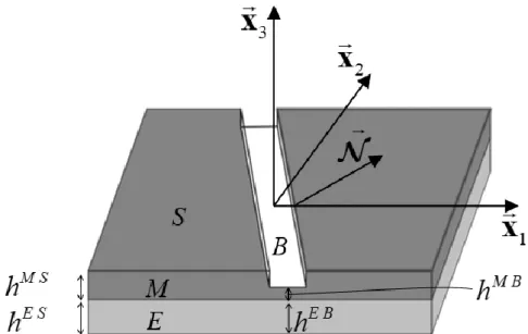
The initial imperfection approach (briefly called M–K analysis hereafter) can be applied to predict the incipience of localized necking in the bilayer (Fig. 2). As will be detailed in Section 2.2., the mechanical behavior of the elastomer layer is assumed to be purely elastic. Consequently, this layer is immune from necking instability (as will be demonstrated in Fig. 7). Hence, to accurately model this problem, it is more convenient to introduce the initial geometric imperfection in the metal layer and not in the elastomer layer. The introduction of this imperfection will ultimately trigger the initiation and development of localized necking in the whole bilayer. Note that this choice of introducing the initial imperfection in the metal layer has already been followed and discussed earlier by Xue andHutchinson (2007, 2008).
-9-
Fig. 2. Schematic representation of the M–K analysis applied to the bilayer.
To clearly develop the main relations of the M–K model, the following notations are adopted:
M B I
h and hM B: initial and current thickness, respectively, of the metal layer inside the band.
M S
I
h and hM S: initial and current thickness, respectively, of the metal layer outside the band.
E B I
h and hE B: initial and current thickness, respectively, of the elastomer layer inside the band.
E S
I
h and hE S: initial and current thickness, respectively, of the elastomer layer outside the band.
Exploiting these notations, the initial geometric imperfection ratio 0 can be defined as
0 1 M B I M S I h h . (9)
The M–K approach is defined by the following four sets of equations:
The equalities between the in-plane velocity gradient tensors in the metal layer and those in the elastomer layer
ˆ ˆ ˆ , ˆ ˆ ˆ .
gM B gE B gB gM S gE S gS (10)
These equalities hold due to the perfect adherence between the two layers.
The kinematic compatibility condition between the safe zone (outside the band) and the band, which can be mathematically formulated as
-10-
ˆ ˆ .
gB gS c (11)
where c denotes the in-plane jump vector.
The equilibrium relation along the interface between the safe zone and the band
ˆ ˆ
ˆ ˆ
. hM S nM S hE S nE S . hM B nM BhE B nE B . (12)
The constitutive model of the metal and the elastomer layer, restricted to the plane dimension, outside and inside the band:
ˆ ˆ ˆ ˆ
ˆ :ˆ , ˆ :ˆ , ˆ :ˆ , ˆ :ˆ .
nM S M S gS nE S E S gS nM B M B gB nE B E B gB (13)
The insertion of relations (13) into the equilibrium equation (12) leads to the following expression:
ˆ ˆ
ˆ
ˆ ˆ
ˆ. hM S M ShE S E S :gS . hM B M BhE B E B :gB. (14)
In other words, Eq. (14) is equivalent to
. ˆS :gˆS . ˆB :gˆB, (15)
where ˆS and ˆB are defined as follows:
ˆS M S ˆM S E S ˆE S, ˆB M B ˆM B E B ˆE B.
h h h h (16)
The jump vector c can be determined by the combination of equations (11) and (15):
1
ˆ . ˆ ˆ : . c g B S B S (17) From Eqs. (12) and (17), it is easy to show that strain localization starts when the magnitude of the jump vector c reaches a sufficiently high value, which suggests that the components ofthe velocity gradient within the band ˆgB become very high as compared to those within the safe zone ˆgS
. In this case, plastic deformation localizes much more quickly in the imperfection zone than in the safe zone. An obvious consequence from Eq. (17) is that the magnitude of vector c will be very large when ˆ .B approaches singularity
ˆ
det . 0
c B . (18)
Comparing Eq. (18) with the bifurcation criterion defined by Eq. (6), it is expectable that the formability limits predicted by the initial imperfection approach tend to their counterparts
-11-
obtained by the bifurcation theory when the initial imperfection ratio 0 tends towards zero.
This statement will be checked in Section 4 on the basis of several numerical predictions.
2.2. Elastomer layer
For the sake of simplicity, exponent ‘E’ referring to the elastomer layer is omitted in the different mechanical variables (for instance, , ˆ) used in this section, with the implicit understanding that these variables are expressed within this layer. The elastomer layer is taken to be incompressible. Hence, the component 33 of the deformation gradient is given by
1 11 33 11 22 1 e f f f . (19)
The mechanical behavior of the elastomer substrate is described by a neo-Hookean model, which is defined by the following relation (Hunter, 1979):
2
2 ,
I v
p
(20)
where p is a pressure, I2 is the second-order identity tensor, is the shear modulus, and v
is the left Cauchy–Green tensor related to the deformation gradient f by
2
. .
v f fT
(21) The combination of the plane-stress condition (2)2 and the incompressibility condition (19)
requires that p takes the form
1 11 e .
p (22)
For the elastomer layer, the in-plane tangent modulus ˆ needed for computing the bilayer tangent modulus through Eq. (7) is determined as follows (Xue and Hutchinson, 2008):
2 1 2
ˆ ˆ I C ˆ C ˆ , (23)
where is a fourth-order tensor. The non-zero components of are given by (Hunter, 1979) 11 11 22 22 11 22 11 22 11 22 2 2 ( ) 2 2 ( ) 1111 2222 2 ( ) 2 2 1122 1212 e e , e e , e , e e . 2 ε ε ε ε ε ε ε ε ε ε μ μ μ μ (24)
In Eq. (23), C1 and C2 are fourth-order tensors reflecting the impact of convective terms on the elastomer tangent modulus and given in index forms as follows:
-12-
1 2 1 1 , , , : , . 2 2 i j k l Cijkl ik lj il kj C ijkl lj ik kj il (25)2.3. Metal layer
All of the mechanical variables and parameters used and computed in this section correspond to the metal layer. To be brief in the subsequent developments, systematic reference ‘M’ to the metal layer is omitted. The mechanical behavior of the metal layer is assumed to be elasto-plastic. To develop the constitutive equations pertaining to the metal layer, the spatial velocity
gradient g, equal to 1
.
f f ,is additively decomposed into its symmetric and skew-symmetric parts, denoted d and w, respectively
g d w (26)
The strain rate d is itself split into its elastic part de
and plastic part dp d de dp
(27) The stress rate is given by the following hypoelastic law relating the time derivative of the Cauchy stress tensor to the elastic strain rate de
: : C d e e (28) where Ce
denotes the fourth-order elasticity tensor defined by two material parameters: the Young modulus E and the Poisson ratio (since elasticity is assumed here to be isotropic).
In the context of the adopted NAFR framework, the plastic strain rate dp
is given by the following relation: , d p p f (29)
where is the plastic multiplier, and p
f is the plastic potential, which is defined by the
Yld2000-2d anisotropic model (Barlat et al., 2003)
1 2 , 2 1 1 2 , ap ap ap p p p p p p p p X X X X X X (30) where coefficient p
a is an exponent describing the degree of sharpness of the plastic potential surface. As to 1, 2
p
X and 1, 2
p
X , they represent the principal values of two linear transformations applied to the stress deviator, which are denoted Sp
and Sp
-13-
,
Sp Lp Sp Lp
(31) The non-zero components of matrices Lp
and Lp
are given as follows:
11 11 3 12 1 12 21 2 21 7 22 22 66 66 2 0 0 2 2 8 2 0 1 0 0 1 4 4 4 0 1 1 , 0 1 0 4 4 4 1 0 3 9 0 2 0 2 8 2 2 0 0 0 3 0 0 0 0 9 p p p p p p p p p p p p p p L L L L L L L L L L 4 5 6 8 . p p p p (32)
The principal values of the transformed stress deviator Sp
, denoted by 1 p X and 2 p X , are expressed as follows:
2 2 11 22 11 22 1 12 2 2 11 22 11 22 2 12 , 2 2 . 2 2 p p p p p p p p p p p p S S S S X S S S S S X S (33)Similar expressions apply for 1
p
X and 2
p X .
The plastic flow is determined by the Kuhn–Tucker constraints
0 0 0,
y iso
F f F (34)
where y
f and iso
denote the yield function and the yield stress, respectively. As the flow rule is non-associated, the yield function y
f is different from the plastic potential p
f . In the
current contribution, y
f has the same form as p
f , defined by Eqs. (30)-(33), but the
corresponding yield parameters 1,..., 8,
y y ay
are different from the potential parameters
1 ,..., 8,
p p ap
, since these two sets of parameters are fitted using different sets of experimental results. Further details on the identification of these parameters will be given in Section 4. The Kuhn–Tucker constraints (34) are supplemented by the expression of the yield stress iso
. In the current investigation, the Hockett–Sherby hardening model is used to express iso
as a function of the equivalent plastic strain eqp by the following relation (Hippke et al., 2017):
e , p q eq m iso p eq A Β (35)where A , Β , m , and q are hardening parameters. The equivalent plastic strain rate p eq
is determined from the plastic work equivalence principle
-14- . d d p y p p p eq eq y f f (36)
Using Eq. (29), Eq. (36) can be transformed as
. p p eq y f f (37) Since p
f is a first-order homogenous function, the application of Euler’s theorem allows the
following relation to be derived:
. p p f f (38)
Hence, Eq. (37) can be reformulated as
. p p p eq y y f f f f (39)
It must be recalled that in the particular case of associated flow rule, p y
f f and p eq
. The constitutive framework described by Eqs. (26)-(39) is complemented here by the derivation of the elasto-plastic tangent modulus Cep
, defined as
: : : . C d C d d C d C g e e e p ep ep (40)In what follows, we provide some details on the computation of Cep
for the case of the NAFR model. When the behavior is elasto-plastic, the Kuhn–Tucker constraints can be equivalently formulated as : 0. y iso y iso p eq p eq f F f (41)
Using Eq. (29), Eq. (40) can be reformulated as
: . C d C d p e e e f (42)
The substitution of Eqs. (39) and (42) into Eq. (41) allows us to derive the following equation:
:C : d 0, y p iso p y iso e p y eq f f f F f f (43) which is equivalent to
-15- :C :d :C : . y y p iso p e e p y eq f f f f f (44)
Hence, can be determined from (44) as
: : . : : C d C y e y p iso p e p y eq f f f f f (45)
Substituting expression (45) of into Eq. (42) allows us to obtain the following expression for : : : : . : : C C C d C d C p y e e e e e y p iso p e p y eq f f f f f f (46)
The comparison between Eq. (40) and Eq. (46) allows identifying the elasto-plastic tangent modulus Cep : : : : C C C C C p y e e ep e y p iso p e p y eq f f . f f f f (47)
Once determined, the elasto-plastic tangent modulus Cep
corresponding to the metal layer is used to determine the expression of the tangent modulus , which relates the velocity gradient to the nominal stress rate tensor (see, e.g., Haddag et al., 2009)
2 1 2 ,
C I C C
ep
(48) where C and 1 C have expressions similar to Eq. (25). 2
The in-plane tangent modulus ˆ is deduced from by using the following plane-stress transformation:
33 33
3333
, , , 1 2 :,
-16-
3. Numerical and algorithmic aspects
3.1. Bifurcation theory
In the context of bifurcation theory, the bilayer remains homogeneous during the deformation and is loaded following the in-plane biaxial stretching and boundary conditions described in Section 2.1. The algorithm developed for the prediction of the formability limits within the bifurcation approach is based on two embedded loops:
For each strain-path ratio ranging between 1 2/ and 1 (with ):
For each time step [ ,t tn n1] (with tn1 tn t), the incremental algorithm detailed in Section 3.3 is applied to solve the constitutive equations in the two layers and then to determine the in-plane analytical tangent modulus ˆ of the bilayer. To apply the bifurcation criterion, the orientation giving the minimum value for
ˆ
det . . over the interval
0 ,90
is searched. If this minimum value is negative, localized necking is predicted and the computation is stopped. As long as the conditions for localized necking are not met yet, the different mechanical variables are updated and the computation is continued for the next time increment.3.2. Initial imperfection approach
When the M–K approach is employed, the homogeneous zone of the bilayer is submitted to the same in-plane biaxial loading and boundary conditions as those prescribed for the whole bilayer in Section 2.1. In this case, the algorithm for the determination of the formability limits is mainly based on three embedded loops:
For 1 2/ to 1 (with ).
o For 0 varying between 0 and 90 (with 0 ).
- For each time increment [ ,t tn n1] (with tn1 tn t), follow the algorithm described in Section 3.3 to integrate the equations corresponding to the initial imperfection approach. The application of this incremental integration scheme is interrupted when the following threshold is reached:
33 / 33 0
M B M S
-17-
The strain component 11M S 11E S
, obtained when the criterion (50) is satisfied, is considered to be the critical strain 11* corresponding to the current band inclination and strain-path ratio .
The necking limit strain 11L corresponds to the minimum of the critical strains 11* over all of the possible angles 0.
The different necking algorithms, presented in Sections 3.1 and 3.2, are implemented in the computing environment Mathematica.
3.3. Incremental algorithms
The aim of the current section is to describe the incremental algorithms used to integrate over a time increment [ ,t tn n1] the different equations that govern the coupling between the constitutive framework defined in Sections 2.2 and 2.3 and the localized necking criteria presented in Section 3.
3.3.1. Bifurcation theory
At tn1, the current in-plane deformation gradient ˆf is updated as follows:
0 . . 0 ˆ ˆ f f n t t t e e (51)
The updated value of ˆf is used in conjunction with the constitutive relations of Section 2.2 to
determine the Cauchy stress tensor E and the in-plane tangent modulus ˆ E in the elastomer layer (without the use of any iterative scheme).
As to the metal layer, the set of incremental equations to be solved are: The plane-stress condition in the metal layer
33 0
M
. (52)
The incremental unknown corresponding to this equation is 33
M . The incremental form of Eq. (29)
. p M p M M M f (53)
-18-
The incremental unknowns corresponding to these equations are the components of
p M
. Under the plane-stress condition, and considering the incompressibility of plastic strain in the metal layer, p M
can be expressed as follows:
11 12 12 22 11 22 0 0 . 0 0 p M p M p M p M p M p M p M (54) The Kuhn–Tucker constraints given by Eq. (34)
0 0 0, M y M iso M M M M F f F (55) where M F depends on y M f and iso M
, which are in turn dependent on M and
p M eq
, respectively. Taking into account Eq. (39), eqp M can be determined once
M
is known. Hence, the unique incremental unknown corresponding to condition
(55) is M. The incremental constraints (55) can be equivalently expressed as a single equality using the Fischer–Burmeister formulation (Fischer, 1992)
2
2
0. M M M M M F F (56)Hence, the governing equations for the metal layer reduce to five scalar equations: Eq. (52) (one scalar equation), Eq. (53) (three scalar equations) and Eq. (56) (one scalar equation). To solve these equations, five scalar incremental unknowns need to be determined: 33
M , 11 p M , 12 p M , 22 p M
, M. The numerical problem for the metal layer is summarized in a set Y of five scalar equations defined as follows:
1 5 33 11 12 22 11 12 22 , , , , . p M p M p M p M p M p M M M M M M M M M M f f f Y (57)
The corresponding incremental unknowns are stored in a vector X
33, 11 12 22
.XM M p M p M p M M (58)
In summary, the incremental algorithm amounts to solving the following non-linear vector equation:
.YM XM 0 (59)
This vector equation is implicitly solved using the predefined function ‘FindRoot’ of
Mathematica. This function is based on an optimized implementation of the Newton–Raphson
algorithm. Once the non-linear system (59) is solved, the various mechanical variables are updated at tn1 and the analytical tangent modulus ˆM
-19-
tangent modulus ˆ is computed by the average relation (7). Once ˆ is computed,
ˆ
det . . is calculated for all possible band orientations, and the occurrence of localized necking is checked.
3.3.2. Initial imperfection approach
When the initial imperfection model is used, the constitutive equations of the elastomer layer are easily solved as explained in Section 3.3.1. As to the metal layer, the set of constitutive equations, very similar to the one formulated in Eq. (57), has to be developed for both zones
,
.YM S XM S 0 YM B XM B 0 (60)
Equation (17) is added to Eq. (60) to obtain a complete set of incremental equations defining the initial imperfection model. The unknowns to be determined from Eq. (17) are the two components of c. After having merged Eq. (17) with Eq. (60), one obtains the following global form of incremental equations:
, Y X 0 (61) where 1 3 1 3 33 11 12 11 12 4 5 4 5 22 22 6 8 1 3 33 11 12 11 , , , , , , , p M S p M S p M S p M S M S M S M S M S M S M S p M S p M S M S M S M S M S p M B p M B p M B M B M B M B M B f f Y Y f Y Y f Y Y
12 9 10 4 5 22 22 1 11 12 1 2 1 1 2 2 , , , ˆ ˆ ˆ ˆ , where U . . . :g , p M B M B M B p M B p M B M B M B M B M B MK B S B S f f Y Y Y Y c U c U (62)and the set of unknown vectors is defined as follows:
1 5 1 5 33 11 12 22 6 10 1 5 33 11 12 22 11 12 1 2 1 2 , , , , , . p M S p M S p M S M S M S M S p M B p M B p M B M B M B M B MK X X X X X X c c (63)The above-described equations (i.e., twelve scalar incremental equations) are strongly non-linear. To solve this set of equations, an iterative scheme, analogous to the one introduced in Section 3.3.1, shall be used. Once the different variables are updated at tn1, the occurrence of localized necking is checked by criterion (50).
-20-
4. Prediction results
4.1. Freestanding metal layer
Numerical predictions are carried out in this section for the AA6016 aluminum alloy. To investigate the effect of the non-associativity degree on the prediction of the onset of localized necking, another aluminum alloy (AA5042) is studied in Appendix A. The parameters corresponding to the Yld2000-2d yield and potential functions for both alloys have been identified in Hippke et al. (2017). Eight experimental results are required to identify the anisotropy parameters of each function:
The yield locus: four stress ratios in four loading directions and the corresponding four
r-values, which are assumed to be equal to 1.0.
The potential function: four r-values in four loading directions and the corresponding four stress ratios, which are assumed to be equal to 1.0.
For comparison purposes, the AFR parameters have been additionally identified, on the basis of stress-ratios and r-values obtained by uniaxial tension tests along 0°, 45°, 90° from the rolling direction and equibiaxial tension state. The identified parameters are displayed in Tab. 1.
Tab. 1. Anisotropy parameters corresponding to the AA6016 aluminum alloy for both plastic flow rules (from Hippke et al., 2017).
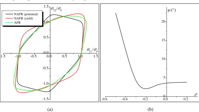
The initial yield and potential loci of the AA6016 aluminum alloy are shown in Fig. 3 (a). To evaluate the non-associativity degree of this alloy, we introduce the non-associativity angle defined as the angle between p /
f
and y /
f
. This angle is determined as follows:
11 11 22 22 . with and . V V V V V V p y p y p y p y p y f f ArcCos f f (64)
When the plasticity model is associated, vectors Vp
and Vy become identical and hence the
angle is equal to 0. We have used the NAFR parameters provided in Tab. 1 to plot in Fig. 3
a 1 2 3 4 5 6 7 8 Yield y f (NAFR) 6 Potential p f (NAFR) 4.5 AFR 4.5
-21-
(b) the evolution of , determined at the onset of bifurcation, versus the negative strain-path ratios . -1.5 -1.0 -0.5 0.0 0.5 1.0 1.5 -1.5 -1.0 -0.5 0.0 0.5 1.0 1.5 NAFR (potential) NAFR (yield) AFR -0.6 -0.4 -0.2 0.00 6 (a) (b)
Fig. 3. Effect of the anisotropy parameters for the AA6016 aluminum alloy on: (a) the yield and potential loci; (b) the non-associativity angle .
The Young modulus and the Poisson ratio of the metal layer are set to 70 GPa and 0.35, respectively. The Hockett–Sherby hardening parameters corresponding to the AA6016 aluminum alloy have been identified by Hippke et al. (2017), as reported in Tab. 2.
Tab. 2. Isotropic hardening parameters for the AA6016 aluminum alloy (from Hippke et al., 2017). A (MPa) B (MPa) m q
352.355 228.655 5.62 0.865
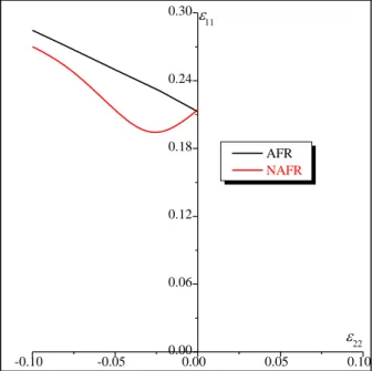
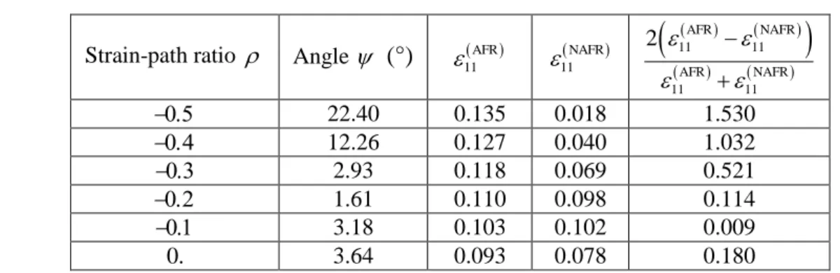
The forming limit diagrams for a freestanding metal layer made of AA6016 aluminum alloy are shown in Fig. 4, as determined by the bifurcation theory. For both plasticity models (namely AFR and NAFR), bifurcation cannot be predicted in the range of positive strain-path ratios ( 0). Hence, only the left-hand side of the FLD is presented in Fig. 4. A first comment is that while the localization limit strains determined by the NAFR model coincide with those predicted by the AFR model for the plane-strain tension state ( 0), the former are always lower than the latter for the other strain paths ( 0)This result can be explained by the destabilizing effect induced by the non-associativity of the plastic flow. Indeed, such non-associativity affects the values of the components of the elasto-plastic tangent modulus
-22- Cep
(see, Eq. (49)), which becomes non-symmetric and, as a consequence, influences the acoustic tensor used in the bifurcation analysis. The difference between the formability limits predicted by both plasticity models is likely to be correlated to the value of the non-associativity angle plotted in Fig. 3 (b): the difference between the predicted limit strains increases with the angle . It must be pointed out that, despite the adoption of the NAFR model, limit strains cannot be predicted by the bifurcation theory for the positive strain-path ratios. This result may be explained by the low degree of non-associativity observed for the AA6016 alloy (as demonstrated in Fig. 3 (b), the yield and potential loci are rather close in shape). To reach bifurcation in the range of positive strain-path ratios, different anisotropy parameters resulting in a higher non-associativity degree should be used (see Appendix A).
-0.10 -0.05 0.000.00 0.05 0.10 0.06 0.12 0.18 0.24 0.30 AFR NAFR
Fig. 4. Forming limit diagrams for the AA6016 metal layer predicted by the bifurcation theory.
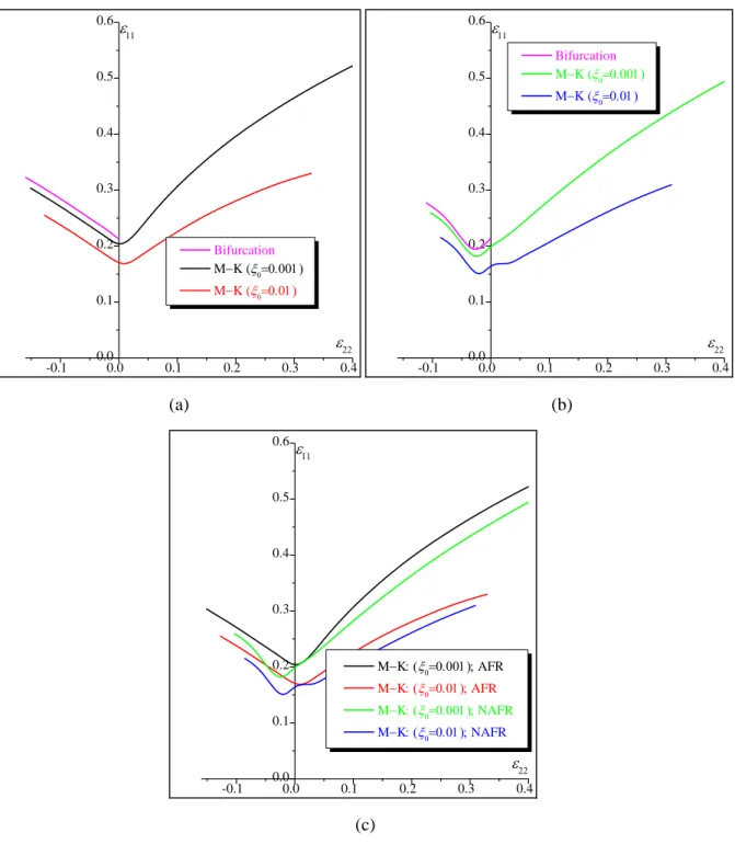
The influence of the initial imperfection ratio 0 on the shape and the level of the FLDs predicted by the M–K analysis is highlighted in Fig. 5 for both plasticity models. It is clear from this figure that even a small amount of geometric imperfection 0 substantially
decreases the limit strains for localization, especially in the range of positive strain-path ratios. Another noteworthy observation is that the limit strains determined by the bifurcation analysis set an upper limit to those predicted by the M–K approach. Indeed, this figure shows that the FLDs predicted by the M–K analysis tend towards the FLD predicted by bifurcation analysis when 0 tends to zero. In other terms, the impact of an initial imperfection is
essentially to move the FLD downwards. This result is expectable taking into account the similitude of the theoretical formulations of the two approaches (bifurcation and M–K), as
-23-
shown in Eq. (17). This result has previously been shown for associated plasticity models (see, for instance, Ben Bettaieb et al., 2015), and it is extended and confirmed here for a non-associated plastic flow rule. Fig. 5 (c) shows that the ductility limits predicted by the coupling between the initial imperfection approach and the associated flow rule (AFR) model are higher than those yielded by the non-associated flow rule (NAFR) model. This result confirms the predictions determined by the bifurcation theory (Fig. 4).
-0.1 0.00.0 0.1 0.2 0.3 0.4 0.1 0.2 0.3 0.4 0.5 0.6 Bifurcation MK ( MK ( -0.1 0.00.0 0.1 0.2 0.3 0.4 0.1 0.2 0.3 0.4 0.5 0.6 Bifurcation MK ( MK ( (a) (b) -0.1 0.00.0 0.1 0.2 0.3 0.4 0.1 0.2 0.3 0.4 0.5 0.6 MK AFR MK AFR MK NAFR MK NAFR (c)
Fig. 5. Impact of the amount of initial geometric imperfection 0 on the shape and the location of the
-24-
4.2. Metal/elastomer bilayer
In this subsection, we carefully analyze the effect of the elastomer layer on the ductility limits of substrate-supported metal layers. For comparison purposes, we consider two combinations of constitutive models: a metal layer modeled by the AFR bonded to a neo-Hookean elastomer substrate, and a metal layer modeled by the NAFR bonded to a neo-Hookean elastomer substrate. In the following results and discussions, the above-defined metal/elastomer bilayers will be briefly called AFR/NH and NAFR/NH, respectively. The material parameters corresponding to the metal layer are the same as those presented in Section 4.1. For the elastomer layer, however, the shear modulus is set to 22 MPa, which corresponds to the shear modulus for polyurea (Amirkhizi et al., 2006).
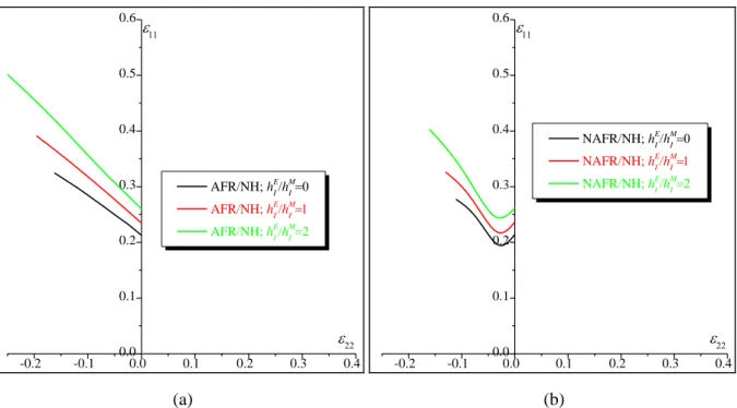
The influence of the elastomer layer and its initial thickness h , relative to that of the metal IE
layer h , on the ductility limits predicted by the bifurcation theory is shown in IM Fig. 6. When
E I
h is set to 0, we obviously recover the bifurcation predictions for a freestanding metal layer
(Fig. 4). It is shown that for both combinations (namely AFR/NH and NAFR/NH), the addition of an elastomer substrate allows moving the FLD monotonically upwards, hence improving the formability of the resulting bilayer. This result demonstrates the major practical benefit of the use of elastomer substrates, as the latter allow delaying the necking limit of functional parts and components.
-0.2 -0.1 0.00.0 0.1 0.2 0.3 0.4 0.1 0.2 0.3 0.4 0.5 0.6 AFR/NH; hEI/hMI AFR/NH; hEI/hMI AFR/NH; hE I/h M I -0.2 -0.1 0.00.0 0.1 0.2 0.3 0.4 0.1 0.2 0.3 0.4 0.5 0.6 NAFR/NH; hEI/hMI NAFR/NH; hEI/hMI NAFR/NH; hE I/h M I (a) (b)
Fig. 6. Impact of the initial thickness ratio E / M
I I
h h on the shape and the location of the FLDs predicted by the bifurcation theory: (a) AFR/NH combination; (b) NAFR/NH combination.
-25-
To better illustrate the improvement in terms of formability when an elastomer layer is bonded to the metal layer, the determinant of the acoustic tensor of the elastomer layer
ˆE . ˆE.
is determined from the expression of the elastomer tangent modulus given by Eqs. (23)–(25):
11 11 11 11 11 11 11 11 11 2 2 1 2 2 3 4 4 3 2 2 2 2 2 2 4 4 ˆ ˆ det det . 3 3 9 2 3 3 E E e e e cose e e cos sin e e sin
(65)
By analyzing the different terms of Eq. (65), one can easily observe that the determinant of
ˆE remains always strictly positive and hence, localized necking can never occur in the elastomer layer alone. Furthermore, Eq. (65) reveals that det
ˆE is proportional to 2( being the shear modulus of the elastomer layer). To graphically illustrate Eq. (65), the determinant of ˆE is plotted for two particular strain-path ratios ( and ) as a function of the band orientation and the major strain 11 in Figs. 7 (a) and (b). On the other
hand, the determinant of the acoustic tensor associated with the metal layer ˆM can be negative for strain-path ratios and , and for some combinations of and 11, as
revealed by Fig. 7 (c) and (d) implying that localized necking in the metal layer is reached for these strain paths. For the strain-path ratio , the determinant of the acoustic tensor ˆM is positive for 110.4, regardless the value of the band inclination , as shown in Fig. 7
(e). Consequently, bifurcation cannot occur in this strain range. In fact, bifurcation is reached for a very high value of 11, not presented in this figure. Note that the associated flow rule
(AFR) has been used to model the mechanical behavior of the metal layer for the predictions presented in Fig. 7. As expected, for the strain-path ratio , the bifurcation angle inclination is around 40° and this inclination is equal to 0° for ratio Unfortunately, it is not possible to provide an analytical expression for the determinant of ˆM , as the constitutive equations corresponding to the metal layer are formulated in an incremental form (unlike the constitutive equations of the elastomer layer, which are formulated in a total form).
As the acoustic tensor of the bilayer ˆ can be derived from the acoustic tensor of each layer by the following averaging rule:
ˆ ˆ ˆ , E E M M E M h h h h (66)
-26-
one can conclude that the addition of an elastomer layer allows increasing the determinant of the bilayer acoustic tensor ˆ , and thus delaying the occurrence of localized necking in the resulting substrate-supported metal layer.
(a) (b)
(c) (d)
-27-
Fig. 7. Evolution of the cubic root of the determinant of the acoustic tensor of each layer: (a)
3 det ˆE for 0.5; (b) 3det
ˆE for 0 (plane-strain tensile state); (c) 3 det
ˆM for0.5
; (d) 3 det
ˆM for plane-strain tensile state ( 0); (e) 3 det
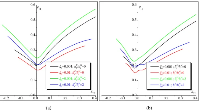
ˆM for 0.1.The positive impact of coating an elastomer substrate on the improvement of the formability of substrate-supported metal layers is confirmed by the results of Fig. 8, where the Marciniak and Kuczynski approach is adopted as localized necking criterion. The occurrence of plastic strain localization may be prevented by perfectly bonding a sufficiently thick and stiff elastomer substrate to the metal layer.
-0.2 -0.1 0.00.0 0.1 0.2 0.3 0.4 0.1 0.2 0.3 0.4 0.5 0.6 0.001; hE I/h M I 0.01; hEI/hMI 0.001; hEI/hMI 0.01; h E I/h M I -0.2 -0.1 0.00.0 0.1 0.2 0.3 0.4 0.1 0.2 0.3 0.4 0.5 0.6 0.001; hE I/h M I 0.01; hEI/hMI 0.001; hE I/h M I 0.01; hEI/hMI (a) (b)
Fig. 8. Impact of the initial thickness ratio E / M
I I
h h on the shape and the location of the FLDs predicted by the Marciniak and Kuczynski approach: (a) AFR/NH combination; (b) NAFR/NH
combination.
5. Conclusions
In the current paper, a comprehensive study is presented to carefully investigate the initiation of localized necking in metal/elastomer bilayers. In particular, the effects of considering a non-associated flow rule in the modeling of the metal layer and of coating an elastomer substrate are specifically highlighted. In this aim, several numerical tools have been developed to predict the onset of localized necking by both the bifurcation theory and the Marciniak and Kuczynski approach. These numerical developments are sufficiently general to
-28-
be employed for other and more elaborate behavior models for both the metal and the elastomer layer. From the presented predictions, key findings can be outlined hereafter:
The main trends for freestanding metal layers and bilayers demonstrate that the lowest limit strains are predicted when the mechanical behavior of the metal layer is modeled by the non-associated flow rule. This result is understandable considering the destabilizing effect induced by the non-associativity of the flow rule (reflected by the difference between the plastic potential and the yield function).
The limit strains determined by the bifurcation analysis can be viewed as an upper limit to the FLDs given by the imperfection approach. This result holds for both constitutive frameworks used to model the mechanical behavior of the metal layer (AFR and NAFR). The gap between the FLDs predicted by the Marciniak and Kuczynski approach and that yielded by the bifurcation theory reduces and tends to vanish as the initial imperfection ratio decreases. This trend, well established for associated flow rule models (see, Ben Bettaieb and Abed-Meraim, 2015), is confirmed here for the adopted NAFR. Considering the similarity in the mathematical formulations of the two localization criteria, this trend is quite expectable: the initial imperfection approach reduces to the bifurcation analysis if the amount of initial imperfection is set to zero. Indeed, as demonstrated by Eq. (18), the onset of localized necking is predicted by the initial imperfection approach when the acoustic tensor associated with the band becomes singular.
Bonding an elastomer substrate to a metal layer substantially enhances the formability of the metal/elastomer bilayer. This observation is shown to be valid whatever the magnitude of the initial geometric imperfection and whatever the flow rule selected to model the plastic behavior of the metal layer.
The numerical tools developed in the present investigation are able to qualitatively and accurately analyze the sensitivity of the ductility of substrate-supported metal layers to the different relevant material and geometric parameters (shear modulus of the elastomer layer, anisotropy and hardening parameters of the metal layer, relative thickness of both layers). These tools can be advantageously used to classify different bilayer components in terms of ductility performance, and then to help in the design of industrial components.