Assumed-strain solid–shell formulation for the six-node finite element SHB6: evaluation on nonlinear benchmark problems

Science Arts & Métiers (SAM)

is an open access repository that collects the work of Arts et Métiers Institute of

Technology researchers and makes it freely available over the web where possible.

This is an author-deposited version published in: https://sam.ensam.eu Handle ID: .http://hdl.handle.net/10985/10358

To cite this version :

Farid ABED-MERAIM, Vuong-Dieu TRINH, Alain COMBESCURE - Assumed-strain solid–shell formulation for the sixnode finite element SHB6: evaluation on nonlinear benchmark problems -2011

Any correspondence concerning this service should be sent to the repository Administrator : archiveouverte@ensam.eu

Science Arts & Métiers (SAM)

is an open access repository that collects the work of Arts et Métiers ParisTech

researchers and makes it freely available over the web where possible.

This is an author-deposited version published in: http://sam.ensam.eu Handle ID: .http://hdl.handle.net/null

To cite this version :

Farid ABED-MERAIM, Vuong-Dieu TRINH, Alain COMBESCURE - Assumed-strain solid–shell formulation for the sixnode finite element SHB6: evaluation on nonlinear benchmark problems -2011

Any correspondence concerning this service should be sent to the repository Administrator : archiveouverte@ensam.eu

Assumed

-

strain solid

–

shell formulation for the

six-node finite element SHB6: evaluation on nonlinear

benchmark problems

Farid Abed-Meraim, Vuong-Dieu Trinh

LEM3, CNRS, Arts et Métiers ParisTech

57078 Metz Cedex 3, France

Alain Combescure

LaMCoS, UMR CNRS 5259, INSA de Lyon 69621 Villeurbanne Cedex, France

Abstract – Because accuracy and efficiency are the main features expected within the finite element (FE) method,

the current contribution proposes a six-node prismatic solid–shell, denoted (SHB6). The formulation is extended here to geometric and material nonlinearities, and focus will be placed on its validation on nonlinear benchmark problems. This type of FE is specifically designed for the modeling of thin structures, by combining several useful shell features with some well-known solid element advantages. Therefore, the resulting derivation only involves displacement degrees of freedom as it is based on a fully 3D approach. Some of the motivation behind this formulation is to allow a natural mesh connection in problems where both structural (shell/plate) and continuum (solid) elements need to be simultaneously used. Another major interest of this prismatic solid–shell is to complement meshes that use hexahedral solid–shell FE, especially when free mesh generation tools are employed. To achieve an efficient formulation, the assumed-strain method is combined with an in-plane one-point quadrature scheme. These techniques are intended to reduce both locking phenomena and computational cost. A careful analysis of possible stiffness matrix rank deficiencies demonstrates that this reduced integration procedure does not induce hourglass modes and thus no stabilization is required.

Key words – solid–shell/assumed-strain method / reduced integration / locking phenomena / nonlinear benchmark problems.

… int n 1 2 x h V 2 3 1 5 6 4 O I.

Introduction

Accuracy and efficiency of finite elements (FE) are the main features expected with the ever-growing resort to FE-based software packages. In particular, for the three-dimensional analysis of structural problems, the development of effective eight-node solid–shell FE has been a major objective over the past decades as revealed by several recently published contributions [1–5]. However, with the advent of free mesh generation tools that do not only generate hexahedrons and in order to automatically mesh arbitrarily complex geometries, the development of prismatic solid–shell elements has been made necessary. Such a solid–shell concept is particularly attractive since it combines in a single formulation the essential useful features of shell FE and the well-recognized advantages of solid FE. Besides the avoidance of complex and elaborate shell kinematics, one of the main interests of the solid–shell approach is to enable a straightforward connection between structural and continuum elements in real-life structures where thin structural components commonly coexist with thicker three-dimensional parts. Note that most of the methods developed earlier were based on the enhanced assumed strain method proposed by Simo and co-workers [6–8], and consisted of either the use of a conventional integration scheme with appropriate control of all locking phenomena or the application of a reduced integration technique with associated hourglass control. Both approaches have been extensively investigated and evaluated in various structural applications, as reported in various contributions [9–15]. The current paper proposes the formulation of a six-node solid–shell FE denoted (SHB6). It consists of a continuum shell derived from a fully three-dimensional approach, in which the displacements are the only degrees of freedom and provided with a special direction designated as the „thickness.‟ The assumed-strain method is adopted together with an in-plane reduced integration scheme using an arbitrary number of integration points – with a minimum of two – located along the thickness direction. The three-dimensional elastic constitutive law is also modified so that a shell-like behavior is intended for the element and in order to alleviate shear and thickness-type locking.

Because reduced integration schemes are known to introduce spurious mechanisms associated with zero energy, an adequate hourglass control is generally needed. An effective treatment for kinematic modes was proposed by Belytschko and Bindeman [1], with a physical stabilization procedure to correct the rank deficiency of eight-node hexahedral elements. As the SHB6 is also under-integrated, a detailed eigenvalue analysis of the element stiffness matrix has been carried out. We demonstrate that the kernel of this stiffness matrix only reduces to rigid body modes and hence, in contrast to the eight-node solid–shell element (SHB8PS) [4, 16], the SHB6 element does

not require stabilization. Nevertheless, we propose

modifications, based on the well-known assumed-strain method [1], for the discrete gradient operator of the element in order to improve its convergence rate.

Indeed, as revealed by numerical evaluations of the SHB6 element, its original displacement-based version, without modification of its discrete gradient operator, suffered from shear and thickness locking. To attenuate these locking

phenomena, several modifications have been introduced into the formulation of the SHB6 element following the assumed-strain method adopted by Belytschko and Bindeman [1]. Finally to assess the effectiveness of the new formulation, a variety of nonlinear benchmark problems has been performed and good results have been obtained when compared to other triangular-based elements available in the literature. In particular, it is shown that this new element plays a useful role as a complement to the SHB8PS hexahedral element, which enables us to mesh arbitrary geometries. Examples using both SHB6 and SHB8PS elements demonstrate the advantage of mixing these two solid–shell elements.

II.

Formulation of the SHB6 finite element

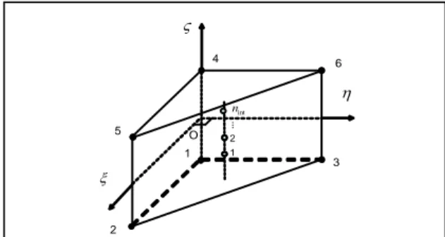
The SHB6 is a six-node prismatic continuum shell with only three displacement degrees of freedom per node. It is provided with a special direction called the „thickness,‟ normal to the mean plane of the triangle. A reduced integration scheme is adopted with at least two integration points along the thickness and only one point in the in-plane directions (see Fig. 1).

Figure 1. Reference geometry of the SHB6 element, and integration points.

Kinematics and interpolation

The SHB6 is a linear, isoparametric element. Its spatial

coordinates x_i and displacements u_i are respectively related to

the nodal coordinates x_iI and displacements u_iI through the

linear shape functions N



N N₁

,

₂

,...,

N₆



as follows:

( , , )

i iI I

x



x N

x h 

,

u

_i



u N

_{iI I}

( , , )

x h 

(1)

Above and hereafter, unless specified otherwise, the implied summation convention for repeated indices will be adopted.

Lowercase indices i vary from one to three and represent

spatial coordinate directions. Uppercase indices I vary from

one to six and correspond to element nodes. The tri-linear

isoparametric shape functions N_I are:

































 









1 1 1 0,1 1 1 , , , with 0,1 2 1 1,1 1 1  x h  x x  h x h  h x  x h   x  h           _{  }  _  _{ }    _{ }   _    _{ }   _   _           N (2)

Discrete gradient operator

Using some mathematical derivations, similarly to the procedure for the SHB8PS development [16], we can explicitly express the relationship between the linear part of the strain field and the nodal displacements. Combining (1) and (2) leads to the following expansion for the displacement field:





0 1 2 3 1 1 2 2 1 2 , , , , , 1, 2, 3 , i i i i i i i u x y z a a x a y a z c h c h i h h x h  h x         







(3)

Evaluating this last equation at the element nodes yields the following three six-equation systems:

0 1 1 2 2 3 3 1 1 2 2 , 1, 2, 3

i ai ai ai ai ci ci i

d s x x x h h (4)

where the six-component vectors d_i and x_i respectively

denote the nodal displacements and coordinates, and vectors s

and h_



1, 2



are given by:

1 2 ( 1, 1, 1, 1, 1, 1) (0, 0, 1, 0, 0,1) (0, 1, 0, 0,1, 0) T T T     











s h h (5)

Let us now consider the derivatives of the shape functions evaluated at the origin of the reference frame:

, = = =0 ( ) 1, 2, 3 i i i Hallquist Form i x _{x h }      N b N 0 (6)

Explicit expressions of vectors b_i can be derived by algebra

together with some useful orthogonality relations:

0 , 0 , 0 , 2 , 1, ..., 3 , =1,2 T T T i i i j ij T T i j                    











b h b s b x h s h h (7)

These orthogonality conditions allow the constants a_ki and c_i

to be determined by scalar products:

3 1 1 where: ( ) 2

,

T ki k i i i T j j j a c_{ }           

























b d γ d γ h h x b (8)

which, combined with (3), lead to the following convenient form for the displacement field:

0 ( 1 1 2 2 3 3 1 1 2 2)

T T T T T

i i i

u a  xb xb xb hγ hγ d (9)

The strain field (i.e., symmetric part of the displacement gradient) is then obtained by differentiating this last equation:

( ) s  u  B d (10) , , , , , , , , , , , , , , , , , ( ) , , x x y y x z z s y x y y x z y z z y x z z x T T x x T T y y T T z z T T T T y y x x T T T T z z y y T T T z z x u u u u u u h h h h h h h h

u

u

u

                              













_{ }





_{ }





_{ }





_{ }

 

















d u d d d b γ 0 0 0 b γ 0 0 0 b γ B b γ b γ 0 0 b γ b γ b γ 0 b h_{,x }T





































γ



(11)

This form of the discrete gradient operator B is very useful

because it allows each of the non-constant strain modes to be handled separately to build an appropriate assumed-strain

field. In addition, it can be shown that the γ_ vectors involved

in this operator satisfy the following orthogonality relations: 0,

T T

j

    

γ x γ h (12)

These conditions will prove to be helpful in the subsequent analysis of stiffness matrix rank deficiencies.

Variational principle

The expression of the weak form of the Hu–Washizu mixed variational principle, as extended to nonlinear solid mechanics by Fish and Belytschko [17], reads for a single finite element:





( , , ) ( ) 0 T T s e e T ext v dv v dv             





v ε σ ε σ σ v ε d f (13)

where  denotes a variation, v the velocity gradient, ε the

assumed-strain rate, σ the interpolated stress, σ the stress

evaluated by the constitutive equations, d the nodal

velocities, fext the external nodal forces, and s( )v the

symmetric part of the velocity gradient. In the simplified form of this principle, as described by Simo and Hughes [18], the assumed stress field is chosen to be orthogonal to the difference between the symmetric part of the velocity gradient and the assumed-strain rate, leading to:

( ) T T ext 0

e

v dv

 ε 



ε σ d f  (14)

Therefore, the discrete equations only require the interpolation of the displacement and the assumed-strain field. The latter is expressed in terms of a B matrix, projected starting from the

( , )x t  ( )x  ( )t

ε B d (15)

Replacing (15) in the variational principle (14), leads to the following expression for the internal forces:

( ) int T e v dv 



 f B σ ε (16)

This formulation is valid for problems involving nonlinear material models, in which σ is a function of the time history of the assumed-strain field and other internal state variables:

( , , ...)



σ F ε  (17)

For linear elastic problems, the element stiffness matrix takes the following simple form:

T e e v dv 



  K B C B (18)

Note that similarly to the SHB8PS element [16], an improved plane-stress type constitutive law is adopted here, to enhance the element immunity with regard to thickness locking.

Hourglass mode analysis

Hourglass mechanisms are spurious zero-energy modes generated by the reduced integration. Therefore, the analysis of hourglass modes is equivalent to the investigation of stiffness matrix rank deficiency. Within a displacement-based

approach, a zero-energy mode is a vector hg that satisfies:

int 1, ...,

(_I) g  ; I  n

B h 0 (19)

We can easily demonstrate that the following



e_i, i1,...,18



vectors are linearly independent, and hence, they form a basis for the vector space of the discretized displacements:

1 2 3 4 5 6 7 8 9 10 11 12 1 13 , , , , , , , , , , , , ,             

 

 

 

 

 

 

 

 

 

 

 

 

 

 

 

 

 

 

 

 

 

 

 

 

 

 

 

 

 

 

 

 

 

 

 

 

 

 

 

 

 

 

 

 

 

 

 

 

 

 

 

 

h e 0 0 s 0 0 x 0 0 e 0 e s e 0 e 0 e x e 0 0 0 s 0 0 x y 0 0 z 0 0 e 0 e y e 0 e 0 e z e 0 0 0 y 0 0 z 2 14 1 15 16 17 2 18 1 2 , , , ,     

 

 

 

 

 

 

 

 

 

 

 

 

 

 

 

 

 

 

 

 

0 0 h 0 0 e h e 0 e 0 e h e 0 0 h 0 0 h

Assuming that vector h belongs to the stiffness kernel, one g

can expand it in terms of the above base vectors:

18 1 g i i i c  



h e (20)

Combining (20), (19), and (11), and taking advantage of orthogonality conditions (7), one obtains:

 

 

 

 

 

 

 

 

 

 

 

 

 

 

 

 

 

4 1, 13 2, 16 8 1, 14 2, 17 12 1, 15 2, 18 5 7 1, 13 1, 14 2, 16 2, 17 9 11 1, 14 1, 15 2, 17 2, 18 6 10 1, 13 1, 15 2, 16 2, I I I I I I I I I I I I I I I I I x x y y z z y x y x z y z y z x z x c h c h c c h c h c c h c h c c c h c h c h c h c c c h c h c h c h c c c h c h c h c h x x x x x x x x x x x x x x x x x x                     

 

₁₈ int 1, ..., I I n c  









































0

Evaluating the above equation at the n_int different integration

points of the SHB6 implies that:

4 13 16 8 14 17 12 15 18 5 7 9 11 6 10 0 0 0 0 0 0 c c c c c c c c c c c c c c c               



















(21) and hence: 1 2 3 5 6 9 g c c c c c c         

 

 

 

 

 

 

 

 

 

 

 

 

 

 

 

 

 

 

 

 

 

 

 

 

 

 

 

 

 

 

s 0 0 y z 0 h 0 s 0 x 0 z 0 0 s 0 x y

This last equation reveals that the kernel of the stiffness matrix only consists of the usual six rigid body modes (three translations and three rotations), and thus no rank deficiency is observed. It should be noted that this formulation of the SHB6

element is valid for any set of n_int integration points located

along the same line xI hI 1₃, I, I1, ...,nint, and

comprising at least two integration points (n_int 2).

Assumed-strain formulation for the SHB6

In this section, the discrete gradient operator B will be

projected onto an appropriate subspace in order to eliminate different locking phenomena; the projected operator will be denoted B . It has been shown that this assumed-strain method is consistent, from a variational perspective, with the Hu– Washizu principle as long as the stress interpolation is appropriately chosen (see Simo and Hughes [18]). However, this variational justification of the assumed-strain method does not provide a general and systematic way to derive adequate assumed-strain fields, and a specific analysis of locking must be conducted for each new element developed based on this approach. For this purpose, we propose a projection scheme that is both effective and simple (see [1] for further details). This consists first of decomposing the discrete gradient

1 2

 

B B B (22)

In this additive decomposition, the first part, B₁, contains the

gradients in the element mid-plane (membrane terms of the deformation) as well as the normal strains, whereas the second

part, B₂, incorporates the gradients associated with the

transverse shear strains:

, , , 1 , , T T x x T T y y T T z z T T T T y y x x h h h h h                





































b γ 0 0 0 b γ 0 0 0 b γ B b γ b γ 0 0 0 0 0 0 0 (23) 2 , , , , T T T T z z y y T T T T z z x x h h h h             





































0 0 0 0 0 0 0 0 0 B 0 0 0 0 b γ b γ b γ 0 b γ (24)

It has been observed, from numerical experiments, that the main locking effects in the SHB6 element originate from the transverse shears. Therefore, we choose an integration scheme that enables us to reduce the associated fraction in the total

strain energy. To this end, matrix B₂ is projected as follows:

2 2

B B (25)

where  is a shear scaling factor. By introducing the additive

decomposition (22) of the B operator into (18) and making

use of projection (25), the stiffness matrix becomes:

1 1 1 2 2 1 2 2 +

T T e e e T T e e v v v v dv dv dv dv           









K B C B B C B B C B B C B (26)

which can be simply written as: K_e K₁K₂. The first term,

1

K , which is not affected by projection, is evaluated at the

integration points as defined above:

int 1 1 1 1 1 1 ( _I) ( _I) ( _I) ( _I) n T T e _I v dv _   J   



  



  K B C B B C B (27)

The second term, K₂, embodies all the projection and reads:

2 1 2 2 1 2 2 T T T e e e v dv v dv v dv 



  



  



  K B C B B C B B C B (28)

The particular choice of additive decomposition (23) and (24) together with projection (25) yields a simplified form for the

second part of the stiffness matrix K₂. Indeed, with these

choices the first two terms, i.e. cross-terms, in the right-hand

side of (28) vanish, and matrix K₂ simply reduces to:

2 2 2 T e v dv 



  K B C B (29)

The identification of the shear scaling factor  in (25) has

been carried out through numerical experiments, and the selected value for this parameter is found to be one half. This value is motivated by extensive testing on a variety of popular test problems, and it leads to reasonably good behavior for the element in most of the test problems that have been tested.

III.

Evaluation on benchmark problems

In this section, the evaluation of the SHB6 element will be carried out through several popular linear and nonlinear benchmark problems. For each test problem, the obtained results are compared with the reference solution from the literature, and when relevant, they are additionally compared with either the solutions given by both the standard three-dimensional six-node prism element PRI6 and the unmodified SHB6 element (i.e., without assumed-strain projection), or those yielded by the hexahedral solid–shell element SHB8PS. For the sake of clarity, the assumed-strain projected version of

the SHB6 will be denoted SHB6bar. The first preliminary linear

test problems are mainly intended to assess the performance of the element in bending-dominated problems and to illustrate the benefit of mixing hexahedral and prismatic solid–shell

elements such as the SHB6bar and SHB8PS. In all numerical

tests, a single element is used through the thickness, unless prescription of boundary conditions requires using two layers of FE. For elastic problems, only two integration points are used, whereas for elastic–plastic tests, five integration points are used through the thickness. In the reported results, the meshes are indicated by the number of subdivisions in each direction (length, width), and the total element number is then doubled, since each rectangle is divided into two triangles.

Buckling of a cylinder under external pressure

In this test, a linear stability analysis of a thin cylinder, which is free at its ends and subjected to a uniformly distributed external pressure, is carried out. This problem also allows the verification of the formulation of the geometric stiffness

matrix

K

_. Indeed, in this linear buckling analysis, the Euler

critical pressure is determined along with the corresponding buckling mode. This critical state is associated with the lowest pressure that makes the global stiffness matrix singular and is classically obtained by solving the eigenvalue problem:



K

e





c

K







X

c



0

(30)

in which



_c is the critical buckling load and

X

_c is the

free A 1 0 0  F 0 1 0   F x y z E = 6.825×107 n= 0.3 R = 10 thickness = 0.04 F = 1 x y z 75°

a) Test geometry and loading b) Initial and deformed configurations

x y z L/2 R e sy m sy m A B C D

P

r E= 2×1011 n= 0.3 R= 2 L= 2 e = 0.02 L/2 R e sy m sy m A B C D Mode 2 z L/2 R e sy m sy m A B C D Mode 4 L/2 R e sy m sy m A B C D Mode 6 x y

The geometric and material parameters are shown in Fig. 2.

Figure 2. Buckling of a thin cylinder under uniform external pressure: geometric and material parameters, boundary conditions and applied loading.

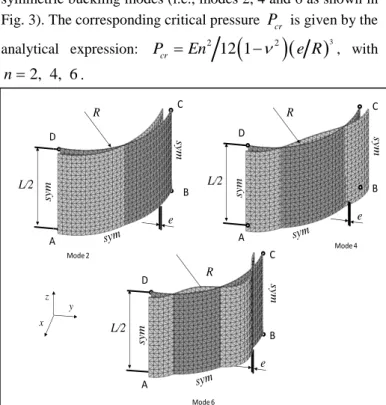
The reference solutions used for comparison are analytical, given by Timoshenko and Gere [19] as well as by Brush and Almroth [20]. Owing to the symmetry of the problem, only one eighth of the cylinder is modeled, and symmetry boundary conditions are applied, which in turn restrict the analysis to symmetric buckling modes (i.e., modes 2, 4 and 6 as shown in

Fig. 3). The corresponding critical pressure

P

_cr is given by the

analytical expression:

P

_cr



En

2

12 1





n

2





e R



3, with

2, 4, 6

n



.

Figure 3. Buckling modes n° 2, 4 and 6; example of a (20×30×1)×2mesh using SHB6 elements for the analysis of one eighth of the cylinder.

The results obtained for the three modes (n2, 4 and

6

)

are reported in Table I in terms of critical pressure, normalized with respect to the analytical reference solution. These reveal

that the assumed-strain version SHB6bar has a better

convergence rate than the SHB6 and PRI6 elements, and represents a significantly improved alternative to the PRI6, which exhibits locking and very slow convergence rate.

TABLE I. NORMALIZED CRITICAL PRESSURE FOR THE THIN CYLINDER SUBJECTED TO UNIFORM EXTERNAL PRESSURE.

Critical

pressure Mesh layout

( ) ( ) ( ) n n cr cr ref

P

P

, (n2, 4, 6) PRI6 SHB6 SHB6bar ( 2)

73260

cr

P



(20×30×1)×2 10.56 1.40 1.25 (20×40×1)×2 6.45 1.21 1.13 (20×50×1)×2 4.55 1.13 1.08 (20×60×1)×2 3.53 1.09 1.05 (20×70×1)×2 2.91 1.06 1.03 ( 4)

293040

cr

P



(20×30×1)×2 10.56 1.42 1.26 (20×40×1)×2 6.44 1.22 1.13 (20×50×1)×2 4.55 1.14 1.08 (20×60×1)×2 3.52 1.09 1.05 (20×70×1)×2 2.91 1.06 1.03 (6)

659340

cr

P



(20×30×1)×2 10.56 1.46 1.28 (20×40×1)×2 6.43 1.24 1.14 (20×50×1)×2 4.54 1.15 1.08 (20×60×1)×2 3.52 1.10 1.05 (20×70×1)×2 2.90 1.07 1.03

Pinched hemispherical shell with mixted FE

This test problem, which is often used to assess the three-dimensional inextensional bending behavior of shells, has become very popular and has been adopted by many authors since it was proposed by MacNeal and Harder [21]. Fig. 4 shows the geometry, loading, and boundary conditions for this elastic thin shell problem (R/t = 250). In this example, a mixture of SHB6 and SHB8PS elements is used, in which the SHB6 elements are located at the top of the hemisphere.

Figure 4. Pinched hemispherical shell problem with a mixture of prismatic and hexahedral elements: the SHB6 elements are located at the top, and the

SHB8PS elements are arranged over an angle of 75°.

Owing to the symmetry of the test, only one quarter of the hemisphere is meshed using a single layer of elements through the thickness and with two unit loads along the directions Ox and Oy. According to the reference solution [21], the

displacement of point A along the x-direction is w = 0.0924. _ref

Note that in order to compare the performance of solid–shell elements to that of standard three-dimensional elements, SHB6 elements are mixed with SHB8PS elements, and PRI6 elements are mixed with their three-dimensional counterpart HEX8, which are the standard, full integration eight-node

R A h P L  B C x y z D R = 2540 L = 254 h = 12.7 = 0.1 E = 3102.75 n= 0.3 = 7 = 6 = 2 y  sat R R C 0 500 1000 1500 2000 2500 3000 0 10 20 30 40 Load

Vertical displacement at the load point A Reference results SHB6 SHB8PS bar L A B C x y z R P E= 10.5×106 n= 0.3125 R= 4.953 L= 10.35 thickness = 0.094 Pmax= 40 000

hexahedral elements. The normalized results reported in Table

II reveal a very good convergence rate when the SHB6bar is

mixed with the SHB8PS, which confirms the interest of mixing hexahedral and prismatic solid–shell elements.

TABLE II. NORMALIZED DISPLACEMENTS AT POINT A FOR THE PINCHED HEMISPHERICAL SHELL PROBLEM: MIXED MESHES.

Number of elements PRI6 + HEX8 SHB6 + SHB8PS SHB6bar + SHB8PS ref w w w w_ref w w_ref 36 0.001 0.703 0.785 100 0.002 0.880 0.960 156 0.004 0.929 0.983

Buckling of a thick elastic–plastic panel

In this nonlinear test problem, the limit-point buckling of a thick elastic–plastic cylindrical panel is investigated. The elastic version of this benchmark has been extensively used in the literature. Here we consider an elastic–plastic version in which both types of nonlinearities, geometric and material, are included. For this new elastic–plastic benchmark problem, we had first to build the associated reference solution. The latter was obtained using Abaqus S4R5 shell elements, for which convergence was achieved with a mesh of 20×20 elements. The geometric and material parameters are given in Fig. 5. The elastic–plastic constitutive equations correspond to the Voce nonlinear saturating isotropic hardening law, which is

associated with the von Mises yield surface

F





_eq

 

Y

0

such that:

Y





_y



R

_sat



1 exp(





C

_R



p

)



, in which



_y is

the initial yield stress,

R

_sat and

C

_R are material parameters,

and



p is the equivalent plastic strain.

Figure 5. Description of the thick elastic–plastic panel benchmark problem; example of mesh with (30×30×2)×2SHB6 FE for one quarter of the panel.

Owing to the symmetry, only one quarter of the structure is modeled. The panel is hinged at its edge BC (mid-surface of the panel), free at its edge CD, and subjected to a concentrated

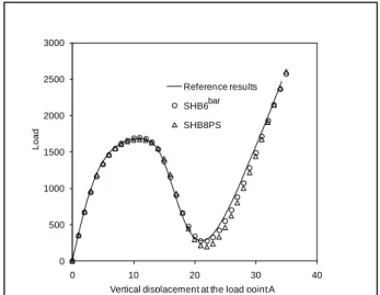
force P at point A along the vertical direction Oz (see Fig. 5). It is noteworthy that this test is very sensitive to the particular location of the prescribed boundary conditions (mid-surface, upper or lower edge), and the corresponding responses show significant differences. Therefore, to reproduce shell boundary conditions (i.e. on the mid-surface), two layers of 3D elements need to be used along the thickness. The results shown in Fig. 6 correspond to the following meshes: 20×20 S4R5,

(20×20×2)×2 SHB6bar, and 15×15×2 SHB8PS FE. In Fig. 6,

the applied load is plotted versus the vertical displacement at the load point A. To be able to capture the snap-through behavior and to follow the curve beyond the limit-point, the Riks path-following strategy has been adopted [22]. It can be observed that the elastic–plastic behavior decreases the first limit load, which is here about 75% of its elastic value. These results are in good agreement with the reference solution obtained with Abaqus S4R5 shell elements, which confirms the ability of the proposed solid–shell FE to predict such critical points and the associated post-buckling response.

Figure 6. Load–deflection results for the thick elastic–plastic panel: comparison between the proposed solid-shell FE and the reference solution.

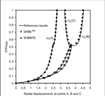
Pull-out of an open-ended cylindrical shell

This test problem consists of an elastic thin cylindrical shell with free edges subjected to a pair of diametrically opposite radial forces. The geometric and material properties as well as the boundary conditions and loading are described in Fig. 7. Only one octant of the cylinder is modeled, due to the symmetry, with a single element along the thickness.

Figure 7. Description of the open-ended cylindrical shell benchmark test: example of mesh with 20×30×1SHB8PS FE for one octant of the cylinder.

0 0.1 0.2 0.3 0.4 0.5 0.6 0.7 0.8 0.9 1 0 0.5 1 1.5 2 2.5 3 3.5 4 4.5 5 P /P m a x

Radial displacements at points A, B and C Reference results SHB6 SHB8PS Uz(A) -Ux(C) -Ux(B) bar

The reference results for this test were given by Sze et al. [23], using the Abaqus shell element S4R with a converged mesh of 24×36 elements. The results shown in Fig. 8 correspond to the

following meshes: 24×36 S4R, (45×45×1)×2 SHB6bar, and

20×30×1 SHB8PS elements, and represent the normalized load versus the radial displacements at points A, B, and C. These reveal that the results of the proposed solid-shell elements are in good agreement with the reference solution.

Figure 8. Load–deflection results for the open-ended cylindrical shell test: comparison between the proposed solid-shell FE and the reference solution.

IV.

Conclusions

A new solid–shell element SHB6bar has been developed and

implemented into the finite element code ASTER. The key idea of this development is the adequate combination of a reduced integration rule with the well-known assumed-strain method. An interesting feature of this approach is the convenient fully three-dimensional framework on which this solid–shell element is based (six-node prism with only three translational degrees of freedom per node). Also it has been shown that no zero-energy modes arise from the adopted reduced integration scheme, and thus no stabilization procedure is required. As

revealed by the benchmark problems, the SHB6bar element

brings significant improvements compared to the standard three-dimensional six-node prismatic element denoted PRI6. The projection using the assumed-strain technique makes the quality of the element even better under combined bending and shearing. This type of element blends naturally with the eight-node hexahedral solid–shell element SHB8PS, thus enabling one to analyze any structural geometry quite easily, which is the main motivation behind the development of the present

SHB6bar element. Recall that meshing arbitrarily complex

geometriesisnotpermittedusingonlyhexahedralelements.

REFERENCES

[1] T. Belytschko and L. P. Bindeman, “Assumed strain stabilization of the eight node hexahedral element,” Comput. Meth. Appl. Mech. Engng., vol. 105, pp. 225–260, 1993.

[2] R. Hauptmann and K. Schweizerhof, “A systematic development of solid–shell element formulations for linear and non-linear analyses employing only displacement degrees of freedom,” Int. J. Num. Meth. Engng., vol. 42, pp. 49–69, 1998.

[3] W. A. Wall, M. Bischoff, and E. Ramm, “A deformation dependent stabilization technique, exemplified by EAS elements at large strains,” Comput. Meth. Appl. Mech. Engng., vol. 188, pp. 859–871, 2000. [4] F. Abed-Meraim and A. Combescure, “SHB8PS a new adaptive,

assumed-strain continuum mechanics shell element for impact analysis,” Computers & Structures, vol. 80, pp. 791–803, 2002.

[5] A. Legay and A. Combescure, “Elastoplastic stability analysis of shells using the physically stabilized finite element SHB8PS,” Int. J. Num. Meth. Engng., vol. 57, pp. 1299–1322, 2003.

[6] J. C. Simo and M. S. Rifai, “A class of mixed assumed strain methods and the method of incompatible modes,” Int. J. Num. Meth. Engng., vol. 29, pp. 1595–1638, 1990.

[7] J. C. Simo and F. Armero, “Geometrically non-linear enhanced strain mixed methods and the method of incompatible modes,” Int. J. Num. Meth. Engng., vol. 33, pp. 1413–1449, 1992.

[8] J. C. Simo, F. Armero, and R. L. Taylor, “Improved versions of assumed enhanced strain tri-linear elements for 3D finite deformation problems,” Comput. Meth. Appl. Mech. Engng., vol. 110, pp. 359–386, 1993. [9] E. N. Dvorkin and K. J. Bathe, “Continuum mechanics based four-node

shell element for general non-linear analysis,” Engineering Computations, vol. 1, pp. 77–88, 1984.

[10] Y. Y. Zhu and S. Cescotto, “Unified and mixed formulation of the 8-node hexahedral elements by assumed strain method,” Comput. Meth. Appl. Mech. Engng., vol. 129, pp. 177–209, 1996.

[11] P. Wriggers and S. Reese, “A note on enhanced strain methods for large deformations,” Comput. Meth. Appl. Mech. Engng., vol. 135, pp. 201– 209, 1996.

[12] S. Klinkel and W. Wagner, “A geometrical non-linear brick element based on the EAS-method,” Int. J. Num. Meth. Engng., vol. 40, pp. 4529–4545, 1997.

[13] S. Klinkel, F. Gruttmann, and W. Wagner, “A continuum based three-dimensional shell element for laminated structures,” Computers & Structures, vol. 71, pp. 43–62, 1999.

[14] S. Reese, P. Wriggers, and B. D. Reddy, “A new locking-free brick element technique for large deformation problems in elasticity,” Computers & Structures, vol. 75, pp. 291–304, 2000.

[15] M. A. Puso, “A highly efficient enhanced assumed strain physically stabilized hexahedral element,” Int. J. Num. Meth. Engng., vol. 49, pp. 1029–1064, 2000.

[16] F. Abed-Meraim and A. Combescure, “An improved assumed strain solid–shell element formulation with physical stabilization for geometric nonlinear applications and elastic-plastic stability analysis,” Int. J. Num. Meth. Engng., vol. 80, pp. 1640–1686, 2009.

[17] J. Fish and T. Belytschko, “Elements with embedded localization zones for large deformation problems,” Computers & Structures, vol. 30, pp. 247–256, 1988.

[18] J. C. Simo and T. J. R. Hughes, “On the variational foundations of assumed strain methods,” ASME Journal of Applied Mechanics, vol. 53, pp. 51–54, 1986.

[19] S. P. Timoshenko and J. M. Gere, Théorie de la stabilité élastique, 2nd

édition, Dunod, 1966.

[20] D. O. Brush and B. O. Almroth, Buckling of bars, plates and shells, McGraw-Hill, New York, 1975.

[21] R. H. MacNeal and R. L. Harder, “A proposed standard set of problems to test finite element accuracy,” Finite Elements in Analysis and Design, vol. 1, pp. 3–20, 1985.

[22] E. Riks, “An incremental approach to the solution of snapping and buckling problems,” Int. J. Num. Meth. Engng., vol. 15, pp. 524–551, 1979.

[23] K. Y. Sze, X. H. Liu, and S. H. Lo, “Popular benchmark problems for geometric nonlinear analysis of shells,” Finite Elements in Analysis and Design, vol. 40, pp. 1551–1569, 2004.