Semantic-preserving mesh direct drilling

Science Arts & Métiers (SAM)

is an open access repository that collects the work of Arts et Métiers Institute of

Technology researchers and makes it freely available over the web where possible.

This is an author-deposited version published in: https://sam.ensam.eu Handle ID: .http://hdl.handle.net/10985/9759

To cite this version :

Ruding LOU, Jean-Philippe PERNOT, Philippe VERON, Franca GIANNINI, Bianca FALCIDIENO, Alexei MIKCHEVITCH, Raphael MARC - Semantic-preserving mesh direct drilling - In: Shape Modeling International, France, 2010-06 - Proceedings of Shape Modeling International - 2010

Any correspondence concerning this service should be sent to the repository Administrator : archiveouverte@ensam.eu

Semantic-preserving mesh direct drilling

Ruding Lou, Jean-Philippe Pernot,

Philippe Véron

LSIS laboratory, UMR-CNRS 6168 Arts et Métiers ParisTech

Aix-en-Provence, France

firstname.lastname@ensam.fr

Franca Giannini,

Bianca Falcidieno

IMATI

Consiglio Nazionale delle Ricerche Genova, Italy

firstname.lastname@ge.imati.cnr.it

Alexei Mikchevitch,

Raphaël Marc

Research and Development Direction Électricité de France Group

Clamart, France

firstname.lastname@edf.fr

Abstract—Advances in modeling of discrete models have allowed the development of approaches for direct mesh modeling and modification. These tools mainly focus on modeling the visual appearance of the shape which is a key criterion for animation or surgical simulation. Most of the time, the resulting mesh quality as well as the semantics preservation capabilities are not considered as key features. These are the limits we overcome in this paper to enable fast and efficient mesh modifications when carrying out numerical simulations of product behaviors using the Finite Element (FE) analysis. In our approach, the modifications involve the resolution of an optimization problem where the constraints come from the shapes of the operating tools and the FE groups (sets of mesh entities) used to support the semantic information (e.g. boundary conditions, materials) contained in the FE mesh model and required for FE simulation. The overall mesh quality, a key point for accurate FE analysis, is guaranteed while minimizing an objective function based on a mechanical model of bar networks which smoothes the repositioning of nodes. Principle of the devised mesh operators is exemplified through the description of a 2D/3D mesh drilling operator. The proposed mesh modification operators are useful in the context of fast maintenance studies and help engineers to assess alternative design solutions aimed at improving the physical behavior of industrial machinery.

Keywords-triangle/tetrahedral meshes; shape semantics; mesh deformation; drilling operator

I. INTRODUCTION

Product behavior numerical simulation has become a mainstream in various engineering domains. It avoids expensive physical experimentations when prototyping and assessing new solutions all along the product lifecycle. It includes the prototyping of maintenance operations which have to be developed and validated as fast as possible to reduce expensive production stops. Thus, it is important to be able to provide rapidly a solution improving production machinery characteristics as well as satisfying multiple safety criteria. Thus, experts must have appropriate numerical tools to rapidly and accurately evaluate different alternative solutions from a physical and/or mechanical view point. Unfortunately, the existing classical methodology for product behavior analysis and solution assessment does not answer to these needs.

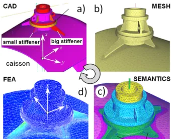
Today, most of the product behavior analyses rely on the following steps: conceptual solution proposal and its detailed design using Computer-Aided Design (CAD) software (Fig. 1. a), complex mesh model preparation for specific behavior studies (Fig. 1. b and c), Finite Element (FE) simulation (Fig. 1. d), results’ evaluation and

optimization loops. During the optimization steps, geometric modifications are generally performed on the CAD models, thus requiring a re-generation of the FE mesh models corresponding to the new solutions. This is done by repeating all the preparation steps necessary for advanced FE analysis: shape adaptation/modification at the CAD level, complex and not fully automatic re-meshing of the CAD models taking into account mesh quality criteria (e.g. generation of free/mapped meshes, creation of sub-meshes having different topologies, a priori adaptive mesh, creation of double entities), re-creation of FE entity groups and re-assignment of semantic information required for FE simulation. In this context we refer to semantic information as all the data necessary for setting up the simulation system. This semantics notably includes Boundary Conditions (BCs), applied forces and pressures, material behavior laws, geometric and mechanical properties. Semantic information is generally associated with the affected mesh elements through the specification of groups. Groups can include any type of mesh elements (e.g. node sets, face and/or tetrahedron sets or a combination of them) and are created by the engineers who graphically select the elements to group.

Figure 1. Mainstream methodology for product behavior analysis and optimization: CAD model modification/adaptation (a); FE mesh generation from CAD data (b); insertion of groups for semantic information, e. g. boundary conditions , pressure areas, specification (c); Finite Element Analysis computation (d). Courtesy by EDF-R&D

This process is clearly time-consuming and there-fore inappropriate for fast analysis of maintenance alternatives. Moreover, in this context, the CAD models are not always available and/or do not fully fit to the reality that can be

measured on the real physical models using 3D scanning techniques. Thus, the creation of the corresponding CAD models starting from scratch would lead to an additional waste of time and should then be avoided as much as possible.

Actually, it is quite clear that going back to the CAD model is not the most efficient method to implement local structural modifications. This is especially true when the model contains numerous mesh groups supporting lots of physical semantic data. For example, the models designed by the EDF (Électricité de France) engineers can contain up to 500 mesh groups. Unfortunately, current commercial CAD systems do not make it possible to automate the process of direct and fast modification of meshes enriched by FE semantic data required for FE behavior simulation of the production machinery, which is crucial for quick studies in the context of maintenance. As a consequence, in prototyping and assessment of structural modifications to improve the production machinery behavior, even small local changes require expensive complete updating of the simulation model.

To overcome these limits, we propose a fast CAD-less prototyping framework working directly at the level of meshes enriched by semantics supported by mesh groups. In this way, the number of steps necessary for FE model preparation stage can be reduced. The idea is to remove the “hard” steps of CAD modification, re-meshing and FE model preparation by bringing necessary local modifications directly onto the meshes while maintaining and potentially propagating the associated semantic data. In this paper, we foresee various operators for direct modification of enriched FE mesh models mechanically tuned (i.e. physically validated). Such an approach is particularly interesting not only for the reuse of tuned and validated FE models but also in the case of so-called “dead” meshes, i.e. FE models whose associated CAD data are unavailable. It also finds interest in the product preliminary design phases where several alternative solutions can be prototyped and compared. Generally speaking, such an approach is useful in all 3D applications where the geometry with associated semantic information necessitates different modifications. Devising such mesh modification operators that take into account and preserve the presence of FE semantic data (i.e. reassign the elements of the modified mesh to the corresponding groups such that the geometrical shape of the groups as well as their boundaries are equal to the original ones) allow the complete re-use of semantically enriched 3D models. Obviously, the preservation and propagation rules are context and semantic dependent. For example, a material law can be directly propagated, whereas for pressure information the correct propagation depends on the context such as the resulting shape characteristics and the cause of the pressure.

The proposed mesh operators simultaneously act at the geometric level, corresponding to the low level mesh elements, and at the structural one, corresponding to the groups expressing the link to the semantics by collecting mesh elements characterized by se-mantic data [15]. The operator behavior is driven by the semantics, including the outer shape of the operands (i.e. of the operated mesh and of the modifying tool) as well as the shape of the groups’

boundaries. This information is transformed into a set of constraints that drive a mesh deformation engine.

The paper is organized as it follows. Section II summarizes some related works. The types of mesh modification operators, their underlying key steps and basic elements are described in section III. Section IV presents a specific operator clarifying the use of the underlying concepts applied to the drilling problem; thus it describes more in details how the general aspects described in section III are exploited and used for this specific operator. Section V provides some results obtained by applying the described operator on semantically enriched mesh.

II. STATE OF THE ART

Today, some commercial and open-source modelers already provide features to work directly on 2D and 3D meshes. They generally offer functionalities to create shapes through the instantiation of simple primitives and successive deformations. Being devoted to gaming and specific applications, they often care neither about the quality of the obtained mesh, nor about the preservation of associated semantic data of different nature (e.g. groups of mesh entities and information related to them). Thus, they cannot modify enriched FE models without lost of semantic data.

At the research level, some works have been proposed both for engineering and surgery applications. Bremberg and Dhondt [4] propose an approach for crack insertion into a volume mesh by computing the intersection between the surface mesh of the crack profile and the skin mesh of the cracked volume mesh. The crack is computed inserting lots of new nodes and faces along the intersection line. Then, the volume is entirely re-meshed using the cracked outer surface of the initial volume mesh. This is not appropriate when working on tuned and enriched models. Moreover, this approach requires the modeling of the crack as a mesh feature and cannot work directly with an analytic definition of the crack equation. In [5], the insertion of a crack into a mesh model is based on the insertion of new nodes along the crack followed by a splitting of the mesh elements. The direct split of elements could be a very fast process that is interesting for real-time visualization of the cracking process. Whereas, from the FE point of view, the resulting mesh is not appropriate because the split elements may have a bad quality in terms of aspect ratio. Similarly, the approach of Turini et al. [16] subdivides the mesh in the surroundings of the cutting tool skin and removes elements intersecting with the cutting tool. Here again, nothing ensures that the resulting mesh owns good shape properties with respect to the FE requirements. The use of Boolean intersection and cut operations between the original model and crack masks have been presented in [7]. Nienhuys and al. [8] describe a cutting algorithm continuously deforming tetrahedra so that the cutting trajectory aligns with faces and edges of the cut model. This method reduces the need to introduce new nodes but can produce degenerate tetrahedra. The approach proposed in [9] allows multiple consecutive incisions of tetrahedra in the crack zone. Each tetrahedron maintains its state information including the number and position of cuts. Multiple cuts are merged, and the affected tetrahedra are subdivided along the cutting plane when a

portion of the mesh is completely severed from the rest. Boolean intersection between acquired and designed geometry is proposed in [10]. A set of intersection algorithms between models of different types is presented. However, the quality of the produced triangles is not controlled in their application domain. Finally, one can quote the work of [6] in which the FE simulation of the crack growth process is performed without re-meshing. In this case, the crack is modeled by an analytic equation which is directly taken into account during the FE analysis. To summarize, various variants of Boolean operations have been proposed. Some apply direct subdivisions which could produce skinny and degenerated elements inadequate from the FE analysis point of view. Some methods also need a full re-meshing with insertion of new nodes everywhere. This is time-consuming and not well-adapted to the modification of tuned mesh models validated by measures performed on the real structure. Finally, these works correspond to purely geometric manipulations which do not take care of potentially attached semantic data.

In this paper, we propose new mesh modification operators exploiting local deformations constrained by shape semantics. The use of a deformation engine avoids the full re-meshing of the tuned and enriched FE 2D/3D mesh models in the surrounding of the eliminated or added parts and ensures the quality of the modified meshes in terms of aspect ratio and conformity. An overview of the basic elements employed in our method is given in the next section; their effective use is illustrated in section IV for the implementation of a specific operator: the mesh drilling.

III. CAD-LESSOPEARTORS’BASICELEMENTS This section introduces the various aspects characterizing the operators of our CAD-less modification platform. They include the specification of the mesh modification type, the adopted shape deformation tool, the shape constraints that can be applied during the deformation process, the group notion and related concepts, the notion of mesh modification interface as well as the characterization of the nodes in its surroundings and the associated deformation constraints.

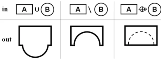
Figure 2. Examples of different categories of operations performed on a mesh A with a tool model B

A. Types of modifications

According to the various mechanical engineering needs, a first set of FE modification operators has been designed; they can be classified according to the following types (Fig. 2): material addition (∪), material removal (\) and crack/contact insertion (ี). These operators directly act on an initial/reference FE mesh (A) with another mesh

or surface primitive (B) used as an operating tool. These operations correspond either to Boolean operations on the reference mesh (for material addition and removal) or as a constrained modification of the reference mesh (for crack/contact insertion). Actually, they can be roughly linked to the classical Constructive Solid Geometry (CSG) operators: union and subtraction of meshes. Crack/contact may be seen as a special case of non-regularized operations. Here, in addition to the geometric modifications, we consider the semantics potentially attached to meshes as a source of information used to constrain the changes. In the future, this initial set of operators will be extended to cover the needs in terms of mesh intersection, mesh blending and so on.

In this paper, we detail the material removal operation for which the operand (B) represents physically a cutting tool removing a set of entities belonging to the mesh (A). Depending on the effect on the topology of the resulting mesh, variants of these operators can be distinguished. When the final tool splits the model (A) in two or more distinct parts, the operation can be considered as a cut, whereas when the operation results in a topological modification, such as a hole insertion, the operation can be considered as a drill. Here, we discuss how to drill 2D as well as 3D meshes to introduce cylindrical through holes in enriched FE meshes (section IV). This operator removes the triangles/tetrahedra totally enclosed in the tool cylindrical surface and uses a deformation engine not only to shape the cylindrical part but also to optimize the aspect ratio of both inner and surrounding triangles/tetrahedra.

B. Mesh deformation tool

In our approach, the mesh modification results from the resolution of an optimization problem defined by a set of linear and non-linear equality constraints, and an objective function ϕ to be minimized (Eq. 1). The unknowns are the positions of the mesh nodes in the surrounding of the area to be modified (section E). They are gathered together in the unknown vector X. The constraints form a constraint vector G constraining some of the nodes position:

⎩ ⎨ ⎧ ϕ = ). ( min , ) ( X 0 X G ₍₁₎

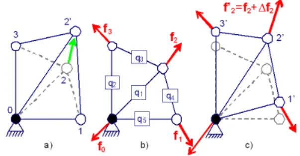
To better control the shape evolution between the constraints, we developed a deformation engine based on the so-called Force Density Method [1]. Given an initial mesh to be deformed (Fig. 3.a), a bar network is built from its nodes (Fig. 3.b): either it can be topologically equivalent to the mesh network or the bar connectivity may differ to generate anisotropic behaviors. Boundary conditions, like prescribed displacements, are specified through a mapping between blocked vertices and nodes of the bar network. Each bar can be seen as a spring with a null initial length and a stiffness qi (more precisely a force density). To preserve the static equilibrium state of bars of length li, external forces fi have to be applied to the endpoints of the bar: fi = qi.li. The set of external forces applied to the initial bar network can be obtained through the static equilibrium equations at each node (Fig. 3.c). At the end, we obtain a set of linear equations between the

node positions X and the external forces applied to them [1]. Being F the vector containing the components of the external forces applied to the nodes free to move, a linear mapping function g between X and F exists:

) (F

X g= (2)

Through this set of equations, we ease the manipulation of the mesh. Fig. 3.a shows that without coupling our bar network to the structure, solely the node 2 is displaced when moving it. If a bar network is coupled to the structure, initial external forces have to be applied to maintain the static equilibrium state (Fig. 3.b). Therefore, a perturbation of the external force applied at node 2 induces a modification of all the free nodes position (Fig. 3.c). If at least one node is blocked, the equation (2) can be inverted to get the external forces as a function of the positions:

) ( 1 _X

F_{= g}− ₍₃₎

In other words, it means that either the external forces applied to free nodes or the free nodes positions themselves can be considered as unknowns of the mesh deformation problem.

Figure 3. Deformation of a network with (c) and without (a) a coupling to the mechanical model (b)

Such a formulation clearly shows the decoupling that exists between:

• the geometric constraints that may be imposed to meshes (e.g. position or specific shape such as a plane). These constraints produce a set of possibly non-linear equations linking directly the position of the free vertices. The resulting constraint vector

G can then be expressed as a function of the

external forces F applied to the free nodes using equation (2);

• the objective function φ to minimize. This is a higher level parameter enabling the specification of various deformation behaviors through the combination of several geometric and/or mechanical quantities relative to the bar network [1]. For example, the minimization of the external forces tends to minimize the surface area and enable a smooth repositioning of the mesh vertices. At the opposite, the minimization of the external forces variations tends to preserve the shape during the deformation; while the minimization of the relative variations of the external forces tends to minimize the discrete

curvature variations over the deformed area. This is interesting to fill in holes in meshes [2].

Actually, such a decoupling enables the specification of an optimization problem with or without constraints. Finally, the objective function φ being often a quadratic form of the unknowns F or X, and since the constraints can be non-linear, a linearization is performed at the first order and the resolution using a Lagrangian becomes iterative.

C. New elementary constraints

To enable the definition of geometric operators based on the adopted deformation engine, new elementary constraints have to be defined to cover most of the needs in mechanical engineering. Therefore at least planar, spherical and cylindrical constraints have to be considered. Let Pm be a mesh node of coordinates (xm, ym, zm), P0 a 3D point of coordinates (x0, y0, z0) and n0 a unit normal vector of components (nx0, ny0, nz0), and the following constraints can be defined on Pm:

• planar constraint so that Pm has to stay on a plane defined by the point P0 and the normal n0:

0 ) ( ) , , ( 0 0 0 m m m = Pm− P ⋅n = pm x y z G (4)

Here, there is just one scalar equation that depends linearly of the position of Pm.

• spherical constraint defined with a sphere

centered in P0 and with a radius R:

0

)

,

,

(

x

y

z

=

−

−

R

=

G

P

P

This non-linear scalar equation can be linearized according to the components of the unknown vector X, or according to the unknown vector F using equations (3). Therefore, at iteration k, the linearized spherical constraint equations according to the unknown positions (xi, yi ,zi) are:

im k m i k sm

_x

_x

x

G

δ

−

=

∂

∂

).

(

2

where δim is the kronecker symbol. Similar equations can be obtained for the y and z coordinates.

• cylindrical constraint defined by a unit vector n0 characterizing its axis and a point P0:

[

(

)

]

0

)

,

,

(

x

y

z

=

−

∧

−

R

=

G

P

P

n

Similarly to the spherical one, the cylindrical constraint can be linearized according to the unknown positions xi as well as yi and zi:

0 0 ] [ 0 0 0 ] [ 0 2 0 2 0 0 ] [ ] [ 0

.

).

.(

.

2

.

).

.(

.

2

)

).(

.(

.

2

n

n

y

y

n

n

z

z

n

n

x

x

x

G

−

δ

+

−

δ

+

+

−

δ

=

∂

∂

where δim is the kronecker symbol. Similar equations can be obtained for the y and z coordinates.

• free-form constraint when the identified shape

introduced constraints. This is done constraining at iteration k the node Pm to move according to the plane defined by the position of Pm at iteration (k-1) and the normal nm to the mesh at this point:

0 ). ( ) , , ( [ ] [ 1] [ 1] ] [ _{= −} − k− ₌ m k m k m m m m k fm x y z G P P n (9)

An equation similar to (6) can easily be obtained. Finally, if the linearization is performed according to the unknown components fix, fiy and fiz of the external forces, the force densities qj inside bars will appear in the linearized equations using equations (2).

D. Groups and related concepts

Groups of mesh entities represent the link between the mesh and semantic information of a physical nature (mechanical modeling, BCs, material properties, etc.) or of shape nature (type of approximate surface/curve). A group collects a set of elementary mesh entities, possibly of different dimensionality, and may be associated with one or more physical or shape semantic data. The semantic information apply to all and only the elements of the associated groups. FE groups useful for FE simulation (to simplify the mechanical modeling, for example) can overlap. This means that a mesh entity can belong to partially overlapping groups. To obtain non overlapping configurations we introduced the notion of Elementary Group (EG) [3]. An elementary group EGk…h is the set of all the mesh entities e such that e belongs to the groups Gh ..k. Thus, a group Gk is formed by one or more elementary groups EGki. In [3] we also present the notion of Virtual Group Boundary (VGB) and we give its description according to different dimension of group entities in the case of 2D and 3D meshes. Roughly speaking, the VGB of a group G is the set of connected mesh elements eb, either belonging to the group or not, that encloses a compact area (volume) in the 2D (3D) mesh whose elements ei are all belonging to G. All the other elements in G that are not in the set of ei and eb are called isolated. The notion of VGB is directly applied and used for the EGs.

This decomposition is useful for setting constraints during the shape modification in order to maintain the association with the semantic data of different nature (geometrical as FE groups, physical as material properties or BCs). Actually, these VGBs permit to identify the volume and area domains of the mesh that are affected by a specific group, thus knowing them allow identifying all the elements that occupy the same volume or area in the mesh. The elementary group boundary and isolated elements should be preserved or deleted if necessary while the internal elements could be free to move inside the VGB or be removed. In the case of insertion of new mesh entities inside the VGB of an EG, the re-assignment of group definition on these new mesh entities can be automatically done to the groups including the concerned EG.

E. Notion of interface

The interface notion gathers together a set of mesh entities, belonging to the reference mesh A, which will be deformed to respect the shape described by the operating

tool B. According to the categories of mesh modification operators presented in the subsection III-A, the interface is computed in different ways.

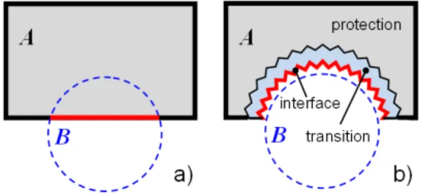
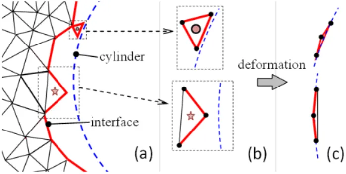
Broadly speaking, for material removal operations, the interface of a mesh of dimension n is the set of elements of dimension (n – 1) adjacent to the elements to be removed from A according to the tool B. In our approach we delete all the elements of dimension n of A which are totally or partially enclosed in B. Fig 4.b shows the interfaces elements identified when drilling an initial rectangle (Fig. 4.a). The interface set identified in this way is further processed to avoid elements of bad quality after the deformation process to fit the shape of B, as it will be deeply described in subsection IV-B for the drilling operation.

Figure 4. Interface elements for a 2D mesh drilling

F. Shape constraints

When performing a mesh modification, several shape constraints of different origin have to be applied. Respecting all the shape constraints leads to a high quality mesh modification that maintains all the characteristics (geometric and mechanical) of the original mesh. The considered shape constraints reflect the:

• mesh skin information relative to surface/edge

types (e.g. cylinder, plane, line, circle or even free form) bounding a 2D/3D FE mesh. This information explicit the fact that a connected set of nodes approximates, at a user-specified accuracy, a given surface or curve primitive (e.g. sphere, cone, cylinder, plane, line, circle). To this aim we have devised a tool [11] partially based on [12] for the detection of surface primitives in 2D meshes possibly corresponding to the external skin of 3D meshes.

• tool characteristics in terms of shapes. For

example, fillet and drilling operations use a cylinder surface tool, analogously the crack insertion may concern the use of a plane for creating the incision. Applying the tool shape constraints guarantees the precise desired shape at the intersection in the resulting mesh.

• group characteristics in terms of shapes. In case

of semantic groups defined on the mesh model, the shape of the group and its virtual boundary have to be considered. The preservation of group shape during the mesh modification is mandatory to avoid reinserting already present semantic information in the mechanically validated mesh. For 2D/3D mesh, if the mesh entity group (nodes and/or edges and/or faces and/or tetrahedra)

occupies a surface/volume area, its virtual group boundary curve/surface shape (node position) is considered. Additionally, in the case of 2D mesh, if the group area is approximating a specific surface type, the group surface shape is directly considered together with the VGB linear shape. This shape information is then used to set constraints for the deformation process. To maintain as much as possible the original FE mesh model, the mesh modification zone is restricted to the area surrounding the operating tool, the interface elements and their neighborhood, called transition zone. In the example of Fig. 4.b, after the rough deletion, the remaining part is divided into a protection zone (gray) and a transition zone (blue). The rough interface is deformed to fit the tool B surface, and only the transition zone nodes are moved so that the variation of density from the preserved mesh elements to the interface elements is smoothed.

Thus, the above described geometric constraints are associated to the interface and neighborhood nodes as it follows:

• nodes on the interface have constrained to stay

on the tool surface;

• nodes of the model boundary that are in the

interface or in the transition zone are constrained to stay on the shape of the model skin;

• nodes in the transition zone will be constrained

to maintain their positions if they are in the virtual group boundaries or to lie on a given surface if they are in a group having associated as shape characteristic that surface;

• all the other mesh nodes are blocked.

Of course, some nodes may belong to several sets and can therefore be assigned constraints relative to both the tool shape and mesh skin shape. When the affected part of the outer skin of the model does not correspond to any surface primitive, we use the model outer skin to assign free-form constraints as introduced in subsection III-C. In the next section we present in details how the concepts presented in these sections are applied in the case of the drilling operation.

IV. MESHDRILLINGOPERATOR

The mesh drilling operation consists of the insertion of a cylindrical through hole. This operation is performed in several steps: identification of the part of the mesh roughly enclosed in the cylindrical volume, rough interface definition, removal of the elements of the enclosed part, deformation constraints setting and interface deformation to match the cylindrical surface of the hole while smoothing the internal nodes positions.

A. Mesh elements classification

As presented in subsection III-A, a drilling corresponds to a particular type of material removal operation; roughly speaking it can be seen as a Boolean subtraction of a cylinder from the FE mesh. The cylinder volume is implicitly defined by its enclosing tool surface. Therefore the first step of this operator requires the identification of the mesh elements to be removed so that the interface subsequently computed subsequently

surrounds the whole cylindrical surface as much as possible.

With this aim, we divide the mesh nodes into two sets,

I and O, which respectively indicate the nodes inside and

outside the cylinder. Then, we gather the mesh entities to be deleted (RT) and to be preserved (KT). In the case of 3D mesh (resp. in case of 2D mesh), we define the set RT as the set of all the tetrahedra (resp. triangles) having at least one node in the set labeled I. For the remaining tetrahedra (resp. triangles) we put them in the set KT. Note that in this way, the mesh elements that are partially inside the cylinder are also defined to be removed. With this choice, the interface completely surrounds the cylinder, thus reducing the possible number of resulting “bad” quality, i.e. roughly flat, tetrahedra in the transition area after the deformation. Additionally, we can note that, as a consequence of the shape of the target surface, i.e. the cylinder, the density of the nodes of the deformed interface will be higher than the one of detected interface.

B. Interface identification and pretreatment

Once we define the mesh elements to be removed, we don’t remove them immediately because original mesh elements are used to retrieve shape information necessary for guiding the deformation process. Nevertheless, we can pre-compute the interface elements. The hole interface is a set ITF of triangles for 3D mesh (resp. edges for 2D mesh) shared by the removed and the kept mesh elements. For 3D mesh (resp. 2D), the set ITF is defined by all the triangles (resp. edges) which are shared by one tetrahedron (resp. triangle) in RT and one tetrahedron (resp. triangle) in KT.

To avoid bad behavior during the successive deformation, we ensure that in case of a 3D mesh (resp. 2D mesh) one tetrahedron (resp. one triangle) in KT is associated with only one triangle (resp. edge) in ITF. Tetrahedra in 3D mesh (resp. triangles in 2D mesh) which do not satisfy this condition will be flattened or flipped due to the deformation of the interface to match the cylinder.

Figure 5. One kept triangle associating with 2 drilling interface edges (a,b) and the corresponding deformed version (c)

For easily understanding the reason an example for the case of a 2D mesh is shown in Fig. 5. The blue dashed arc in Fig. 5.a represents the section of the cylinder so that the axis of the cylinder is perpendicular with the picture. Fig.

5.a shows the elements of KT of the operated triangle mesh; for sake of clarity, the elements in RT are not drawn. The red edges constitute the interface. In this example, the triangle tagged by a pentagram has 2 edges belonging to the interface and the triangle tagged by a circle has 3 edges belonging to the interface. Configurations with triangles having 3 interface edges rarely happen except for the case of flipping triangles or numerical error. Fig. 5.b shows a zoom of these two problematic configurations, and Fig. 5.c shows their possible shapes after the deformation of the interface. The three nodes of the triangles are on the circle, and the triangles are flattened and flipped. So, it is necessary to prevent such configurations.

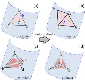
Figure 6. Examples of a kept tetrahedron associating with 2 drilling interface triangles (a) and with 3 drilling interface triangles (c) and their corresponding deformed versions (b, d)

Fig. 6 illustrates a configuration where a tetrahedron is associated with 2 or 3 interface triangles. It could rarely happen that a tetrahedron is associated with 4 interface triangles. The tetrahedron abcd shown in the Fig. 6.a is associated with two interface triangles ∆abc and ∆adc. Fig. 6 .b presents the deformation result when all four nodes are on the cylinder (cutting tool). The dihedral angle between the two interface triangles is θ that is smaller than 180° before the deformation and bigger than 180° after the deformation. This tetrahedron is flattened and flipped. Fig. 6 .c corresponds to a case where the problematic tetrahedron associates with 3 interface triangles ∆abc, ∆adc and ∆bcd. Fig. 6 .d shows the result of the deformation. The node c is close to the triangle ∆abd and this node is at different sides of the triangle ∆abd before and after the deformation. This tetrahedron is also flattened and flipped. Similarly a tetrahedron associated with 4 interface triangles will be also flattened.

To prevent such configurations, in case of a 2D mesh, the solution is to remove the two (resp. three) concerned interface edges from the interface set ITF and add the third (resp. no) edge of the problematic triangle to ITF. At

this stage, no mesh elements are removed, therefore while changing ITF we actually move this triangle from the KT to RT. Fig.7 shows how to apply the solution on the example illustrated in Fig. 5. The problematic triangles shown in Fig.7.a are removed from the set KT (Fig.7.b), the five initial interface edges on those two triangles are also removed from the interface and the third edge of the triangle tagged by a pentagram is added into the interface. The triangle tagged by a green heart symbol is the one associated with the newly added interface edge.

Figure 7. Drilling interface updating for case of kept triangle associating with 2 interface edges

In case of a 3D mesh, the problematic tetrahedra associated to two or more interface triangles, are deleted, i.e. moved from the set KT to the set RT. Then the interface triangles are removed from the interface set, and are substituted by the other triangle(s) of the tetrahedron.

Figure 8. Example of tetrahedron split for a particularly critical interface configuration (a), its split version (b), its original adjacent tetrahedrons (c) and the updated adjacent tetrahedrons

In case of a tetrahedron associated with two interface triangles, this approach is applied only when the remaining tetrahedra do not have in turn two interface triangles. In this case, which rarely occurs in the examples we tested, we split the concerned tetrahedron such that it is substituted by two new tetrahedra having only one triangle in ITF. This is done by splitting the edge not shared by the two interface triangles and joining the new node to the other two non adjacent vertices, thus a new

triangle is obtained by considering these two new edges and the one shared by the interface triangles. In the example of Fig 8 the two interface triangles are ∆acd and ∆abc, thus the edge split is bd, Fig. 8.a. Then, the new edges ao, co and po are created. Thus, the original tetrahedron abcd is split into the two tetrahedrons abco and acdo which have only one interface triangle. As a consequence all the tetrahedra adjacent to the initial edge bd, see Fig. 8.c, have also to be split as shown in Fig 8.d

C. Constraint definition and deformation

Once the elements of the interface set ITF are identified, the transition zone can be defined. All the nodes on the interface and the nodes in the transition zone will move for achieving the drilling surface taking into account mesh quality aspects. As previously said, the goal of the transition zone is to improve the mesh quality to make the variation of density from the interface to the unmodified mesh progressive. The transition zone nodes are the i-th _{neighborhood of the ones associated with the}

ITF elements. The bandwidth “i” can be specified by the

user or computed automatically. When automatically computed, its value is obtained by dividing the biggest distance between the interface nodes and the cylinder by the mean edge length. This gives an idea of how much the nodes have to move to achieve the target shape in relation with the density of the mesh. The bigger this value is the smoother the transition will be if we consider a larger neighborhood, and the better the quality of the mesh will be.

To assign the various constraints to the interface and transition nodes, the different shape information indicated in subsection III-F needs to be derived as well as the classification of the concerned nodes.

At first, the mesh boundary elements of the transition area are detected. For 3D mesh, the boundary is the connected set of triangles that associate only with one tetrahedron of the mesh. Similarly, for 2D mesh, the boundary is the connected set of edges that associate with only one triangle and the “body” is the set of all the triangles in the mesh. As mentioned in subsection III-F in the case of 2D mesh, not only the curve shape of the boundary but also the surface shape of the 2D mesh body are taken into account during the deformation. All this shape information is computed with all original mesh entities before the deletion of the RT elements. Then, the shape of the elementary groups is computed for all those present in the original FE mesh affecting elements in the interface and transition area. Once all important shape information is computed, the mesh elements in the set RT are removed from the mesh. Finally, the nodes on which to assign the constraints are identified and classified as:

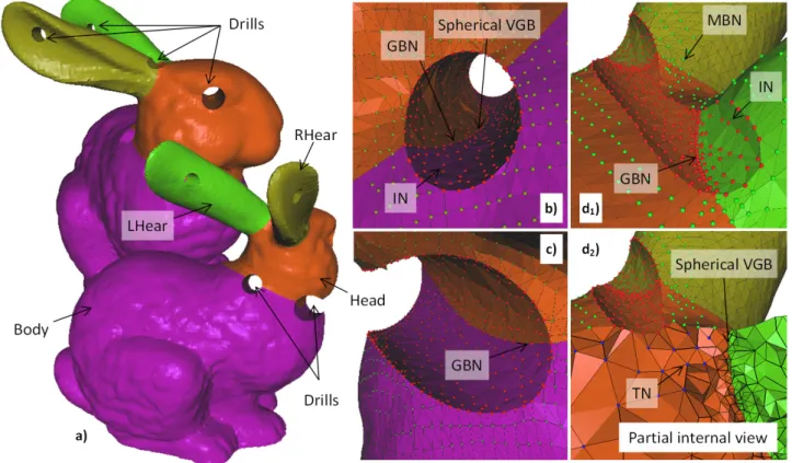
• IN: nodes associating to the interface elements,

• TN: nodes in the transition zone, free to move

during the deformation,

• MBN: nodes on the boundary of the mesh,

constrained,

• GBN: nodes on the boundary of the groups.

At this point it is possible to set the boundary conditions and shape constraints, as specified in subsection III-F. Finally, the deformation process is applied. Since the cylinder constraint, applied to the IN nodes and possibly on the MBN and GBN depending on their respective shapes, is not linear, the minimization step could be applied several times with lineralized constraints.

V. RESULTS

This section illustrates some results relative to the application of the mesh drilling operator on both 2D and 3D meshes.

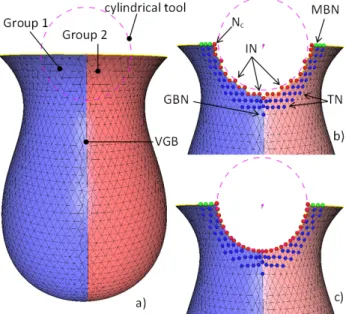
Figure 9. Cylindrical drilling in a 2D mesh containing two groups (a), result of the node removal and classification (b), final result of the drilling operation (c)

First, the cylindrical drilling operator is applied on the triangle mesh of a vase in which two groups of triangles are present and correspond to the two quarters of the vase (Fig. 9.a). The VGBs thus defined come from the intersection between the half-vase and a plane crossing the vase axis. The first step aims at removing all the triangles that are completely inside the cylindrical volume defined by the tool’s axis and its radius (Fig. 9.b). Constraints are assigned to the various nodes surrounding the identified interface. Since it is a 2D triangle mesh, all the free nodes are constrained to stay on the half-vase skin using free-form constraints as described in subsection III-C. In addition, IN nodes, colored in red in Fig. 9.b, have to stay onto the cylindrical tool, GBN nodes have to stay on the identified VGB and MBN nodes, colored in green, have to stay on the mesh boundary. Thus, the node Nc is constrained to stay on the mesh skin, on the mesh boundary and on the cylindrical tool. A bar network is coupled to the mesh nodes and edges surrounding the interface and initial external forces are computed so that the mesh is in a static equilibrium state. To smooth the nodes distribution over the mesh, the minimization of the external forces applied to the nodes is used. The resolution of this optimization problem produces a deformed model that satisfies the constraints while relaxing the position of

the TN nodes solely constrained by the shape of the mesh skin (Fig. 9.c). The aspect ratio of the resulting triangles [17] is good and has even been improved in the present case. Table 1 summarizes the information relatives to each example. We can see the number of holes created, the number of unknowns and the initial and final aspect ratios for each example.

TABLE I. TETRAHEDRON OR TRNIAGLE MEAN ASPECT RATIO [17]

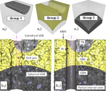
Meshes Criteria Vase (Fig. 9) Cube (Fig. 10) Meca (Fig. 11) Bunny (Fig. 12) Nb. holes 1 1 9 5 Unknowns 87 1932 7336 8150 Qinit 0.908 0.708 0.640 0.663 Qfinal 0.922 0.699 0.623 0.655 In the second example, the cylindrical drilling operator is applied on a cube-like tetrahedral mesh semantically enriched with three groups (Fig. 10.a). Also in this example the groups include all the mesh nodes and are overlapping only at their boundaries. Here, the definition of the groups is such that the resulting boundary between groups 1 and 2 is cylindrical and the boundary between groups 2 and 3 is spherical. As a consequence, some nodes are constrained to stay on the cylindrical tool, some others on the spherical VGB, some on both, and so on. For 3D mesh, TN nodes are completely free to move inside the volume. Here, MBN nodes have to stay on the faces of the cube that have been identified using [11]. The final solution results from the use of the minimization of the external forces applied to the bar network coupled to the nodes and edges surrounding the IN nodes.

Figure 10. Cylindrical drilling in a 2D mesh containing two groups (a), result of the node removal and classification (b), final result of the drilling operation (c)

Such an approach enables the insertion of several holes in one deformation step as illustrated on Fig. 11 where 9 holes have been obtained in one deformation step.

Finally, the drilling operator has been applied several times on the Stanford Bunny to which four groups have been associated so that the resulting VGB are spherical (Fig. 12). Here again, the resulting shapes satisfy the

constraints arising from the shape of the tool, the shape of the VGB as well as the shape of the outer skin of the Bunny, thus preserving the associated semantics.

Figure 11. Cylindrical drilling in a 2D mesh containing two groups (a), result of the node removal and classification (b), final result of the drilling operation (c)

VI. CONCLUSION

In this paper, we propose a deformation-based direct mesh modification framework that aims at directly manipulating mesh models while preserving the mesh quality and the associated semantic information. The framework has been formalized and the types of the foreseen operations as well as the underlying concepts and parameters have been specified. All the important shape characteristics are converted in a set of node constraints used as inputs of our deformation engine that is based on a linear mechanical model of bar network coupled to the nodes and edges of the mesh. The devised approach can be applied to both 2D and 3D meshes.

Our approach differs from existing ones providing a different perspective of applying Boolean-like operations on 3D meshes specifically targeted to guarantee not only geometric (the shape of the mesh) but also semantic information preservation during the shape modification. Additionally our approach is deformation-based in the sense that meshes are only locally changed by repositioning existing nodes without any re-meshing or new elements insertion (except from those directly coming from the added mesh in case of union operations). Main limitations of the methods are related to the need of having enough nodes to obtain the wished deformation according to the identified constraints and quality requirements. For drilling operations, this includes also a certain minimum density relative to the model shape and the relative radius. A feasibility evaluation has to be performed before applying the deformation by checking if there are enough nodes to archive the wished shape. Alternatively an a posteriori quality check could be performed and, if needed a very local re-meshing could be foreseen to avoid infrequent but possible skinny triangles. However, in the context of FE models, the density is usually so high that the proposed approach is very often applicable directly (i.e. without adding new elements using mesh refinement techniques)

To show the capability of the framework, the drilling operator has been presented and tested on several examples both for mechanical engineering and computer graphics applications.

Future works concern the extension of the toolbox to other operators acting on 3D enriched meshes: intersection, union, blending of 3D tetrahedral meshes. The definition of tools having more complex user-specified outer shapes is also envisaged, as well as the possibility to let the user moving his/her tool over the 3D mesh to shape it interactively.

ACKNOWLEDGMENTS

This work is partially supported by the Research and Development direction of the EDF Group, and it is partially carried out within the scope of the FOCUS K3D project supported by the European Commission [13].

REFERENCES

[1] J-P. Pernot, B Falcidieno, F Giannini, J-C. Léon, Shape tuning in Fully Free-Form Deformation Features, J. of Computing and Information Science in Engineering, 5(2):95-103, 2005.

[2] J-P. Pernot, G. Moraru, P. Véron, Filling holes in meshes using a mechanical model to simulate the curvature variation minimization, J. Computers & Graphics, 30 (6): 892-902, 2006. [3] R. Lou, F. Giannini, J-P. Pernot, A. Mikchevitch, B. Falcidieno, P.

Véron, R. Marc, Towards CAD-less finite element analysis using group boundaries for enriched meshes manipulation, Proc. of the ASME Int. Design Eng. Tech. Conf. & Computers and Information in Eng. Tech. Conf., DETC09-CIE86575, San Diego, USA, 2009. [4] D. Bremberg, G. Dhondt, Automatic crack insertion for arbitrary

crack growth. Int. J. of Engineering Fracture Mechanics, 75:404– 416, 2008.

[5] M. Schoellmann, M. Fulland, H.A. Richard, Development of a new software for adaptive crack growth simulations in 3D structures, Int. J. of Engineering Fracture Mechanics, 70(2):249-268, 2003. [6] N. Moes, J. Dolbow, T. Belytschko, A Finite Element Method for

Crack Growth Without Remeshing, Int. J. for Numerical Methods in Engineering, 46(1):131-150, 1999.

[7] A. Martinet, E. Galin, B. Desbenoit, S. Akkouche, Procedural modeling of cracks and fractures, Int. Conf. on Shape Modeling and Applications, pp. 346-349, 2004.

[8] H-W. Nienhuys, A. F. van der Stappen, Sup-porting cuts and finite element deformation in interactive surgery simulation, Technical Report, Univer-siteit Utrecht, 2001.

[9] K. Kundu, M. Olano, Tissue Resection using Delayed Updates in a Tetrahedral Mesh, Proc. of Medicine Meets Virtual Reality 15, Eds. J.D.Westwood and al., IOS Press, Netherlands, 2007. [10] P. Yang, and X. Qian, Direct Boolean intersection between

acquired and designed geometry, Computer-Aided Design, 41(2):81-94, 2009.

[11] A. Bargier, F. Giannini, R. Lou, J-P. Pernot Surface primitive recognition, Technical Report CNR-IMATI 08/09.

[12] M. Attene, B. Falcidieno, M. Spagnuolo, Hierarchical mesh segmentation based on fitting primitives. Visual Computer, 22 (3): 181 - 193. Springer-Verlag, 2006.

[13] Foster the Comprehension and Use of Knowledge intensive 3D media, FP7 Coordination Action, www.focusk3d.eu

[14] SALOME®. Open Source Integration Platform for Numerical Simulation, www.salome-platform.org.

[15] Aim@Shape 2004-08. European Network of Excellence, Key Action: 2.3.1.7, Semantic-based knowledge systems, FP6, www.aimatshape.net.

[16] G. Turini, F. Ganovelli, C. Montani, Simulating drilling on tetrahedral meshes, Proceedings of Eurographics Conference, pp. 127-131, 2006.

[17] Q. Du, D. Wang, Tetrahedral mesh generation and optimization based on centroidal Voronoi tessellations. Int. J. Numer. Methods Eng., 56(9): 1355–1373, 2003.