Science Arts & Métiers (SAM)
is an open access repository that collects the work of Arts et Métiers Institute of
Technology researchers and makes it freely available over the web where possible.
This is an author-deposited version published in:
https://sam.ensam.eu
Handle ID: .
http://hdl.handle.net/10985/8651
To cite this version :
Nicolas MEALIER, Frédéric DAU, Laurent GUILLAUMAT, Philippe ARNOUX - Reliability
approach for safe designing on a locking system - Probabilistic engineering mechanics - Vol. 25,
n°1, p.67-74 - 2010
Any correspondence concerning this service should be sent to the repository
Administrator :
[email protected]
Reliability assessment of locking systems
N. Mealier
a, F. Dau
a,∗, L. Guillaumat
a, P. Arnoux
baLAMEFIP, Esplanade des Arts et Metiers, 33405 Talence cedex, France bCEA/CESTA BP 2, 33114 Le Barp, France
Keywords: Reliability Safety system Monte Carlo FORM/SORM method Experimental design Response surface
a b s t r a c t
The aim of this work is to predict the failure probability of a locking system. This failure probability is assessed using complementary methods: the First-Order Reliability Method (FORM) and Second-Order Reliability Method (SORM) as approximated methods, and Monte Carlo simulations as the reference method. Both types are implemented in a specific software [Phimeca software. Software for reliability analysis developed by Phimeca Engineering S.A.] used in this study. For the Monte Carlo simulations, a response surface, based on experimental design and finite element calculations [Abaqus/Standard User’s Manuel vol. I.], is elaborated so that the relation between the random input variables and structural responses could be established. Investigations of previous reliable methods on two configurations of the locking system show the large sturdiness of the first one and enable design improvements for the second one.
1. Introduction
Integration of uncertainties in a complex system to evaluate the failure probability as regards dreaded events remains a question of great interest. It constitutes an invaluable help in taking risks when dimensioning structures which can avoid the use of excessive safety coefficients. In the present paper, a reliability methodology is proposed to evaluate the failure probability Pfof a
locking system. As the failure probability is generally not obtained by experiments, this methodology is based on an approach which combines both mechanical and reliable analyses using modelisation and reliability tools. This approach has already been investigated in numerous different engineering fields: nuclear [3, 4], offshore [5,6] and civil engineering [7].
The locking system description and specifications are first presented. Two variants of the system, denoted system A and
system B, are considered.
Secondly, the methodology to achieve the failure probability is detailed: Experimental Design (ED), Finite Element Simulations
(FESs), Response Surface (RS) and Reliability Analysis (RA) compose
the successive stage of this methodology. Each of them will be developed and justified. Interest in using first ED, FES, RS and coupling between FES and RA will also be explained.
The failure probability level and the statistical sensitivity of the input variables obtained with reliability tools are compared and
∗Corresponding author. Tel.: +33 5 56 84 53 35; fax: +33 5 56 84 53 66.
E-mail address:[email protected](F. Dau).
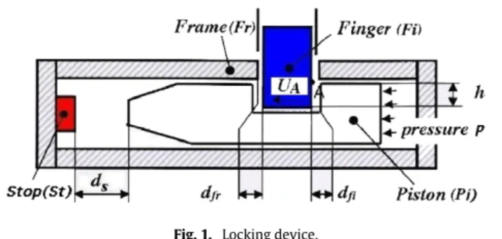
Fig. 1. Locking device.
discussed in the results part for both system A and system B. Finally, conclusions are given underlining interests of this kind of approach in designing complex systems.
2. The locking system
2.1. Description and specifications
The device studied is integrated in a pneumatic dispenser. It is composed of four distinct parts, as illustrated inFig. 1. The Finger
(Fi) must prevent the Piston
(
Pi)
displacement up to the Stop (St) inthe case of untimely setting pressure p in device. This is precisely the feared event to take into account in the reliability analysis.
ds is the distance between (St) and (Pi), dfr represents the
existing gap between (Fr) and (Fi), dfi denotes the existing gap
between (Fi) and (Pi) and h stands for the distance between (Pi) and
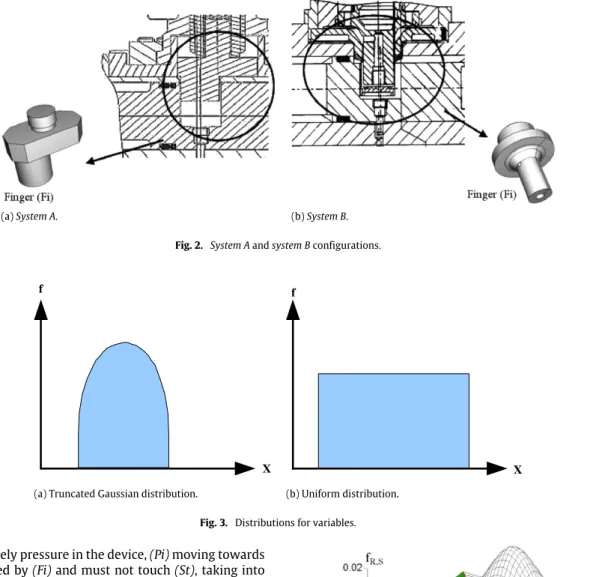
(a) System A. (b) System B.
Fig. 2. System A and system B configurations.
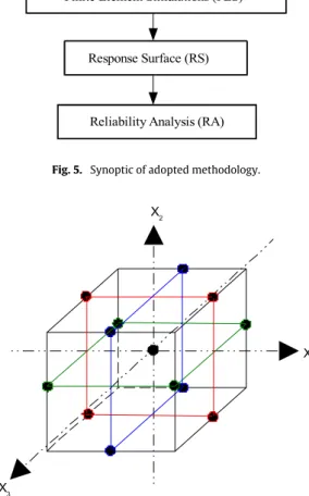
f
X f
X
(a) Truncated Gaussian distribution. (b) Uniform distribution.
Fig. 3. Distributions for variables.
In the case of untimely pressure in the device, (Pi) moving towards
(St) must be stopped by (Fi) and must not touch (St), taking into
account ds, dfi and dfr distances but also a displacement UA at
position A (seeFig. 1) due to the (Fi) deformation.
The specification in terms of failure probability as regards the feared event ‘(Pi) touches (St)’ is 10−4. That is to say, in 104events,
the feared event must occur less than one time!
Two variants of the system,Fig. 2a, b, respectively called system
A and system B, are studied. The difference between the two
systems only concerns (Fi) geometry.
2.2. Reliability problem statement
The reliability problem statement consists in traducing the feared event in a mathematical way in order to be able to evaluate the failure probability Pf as regards this event. Classically, a
performance function G is introduced. It is defined as the difference between a strength function R and a loading function S so that
(
G=
R−
S) ≤
0 corresponds to the failure of the system. The limit case when G=
0 corresponds to the limit state of the system. For this problem, the performance function G is expressed byG
(
ds,
dfi,
dfr,
h) =
ds−
(
dfi+
dfr+
UA)
(1)with displacement UA
=
UA(
dfr,
h,
p)
depending on the materialproperties, loading and boundary conditions, and where dsstands
for R and
(
dfi+
dfr+
UA)
stands for S. At this stage, S is implicitlydepending on the parameters dfi, dfrand UA.
The uncertainties involved in the present system concern parameters ds, dfi, dfr and h but also the pressure p. In default
of knowing real distributions for those parameters, we choose
Fig. 4. Density of joint probability.
truncated Gaussian distributions for the geometric parameters ds, dfi, dfrand h, avoiding in this manner non-physical values. On the
other hand, an uniform distribution is chosen for the imposed parameter p,Fig. 3a-b. So, no preferential values are expected in the fixed range (800–1200 bar). These distributions are supposed to be realistic in this application.
InFig. 3a, x stands for ds, dfi, dfrand h. In bothFig. 3a-b, f denotes
the density of probability for the respective variables.
Mathematically, the failure probability can be classically expressed by
Pf
=
Z
G≤0
fR,S
(
x1, . . . ,
xn)
dx1. . .
dx2,
(2)where fR,S represents the density of joint probability for R and S,
Fig. 4, and xistands for variables, i
=
1,
n.Finally, the reliability problem can be summarized as follows:
Evaluate Pf from Eq.(2)as regards the feared event defined by
Fig. 5. Synoptic of adopted methodology.
Fig. 6. 3D drawing of the Box–Behnken matrix.
Unfortunately, the calculation of Pf from Eq.(2)is not so easy,
and that is why approximated methods are used for this.
3. Methodology for this work
Considering the five variables as explained in previous section and due to system complexity, it is not realistic to assess the failure probability directly with the Monte Carlo method by using experimental or numerical ways due to the prohibitory number of trials. So, a specific but classical methodology involving experimental design and finite element simulations to elaborate the Response Surface (RS) for reliability analysis [8–10] is developed. Such a meta-model avoiding Finite Element (FE) calculations is not time consuming.
Different stages of this methodology,Fig. 5, are detailed in this section.
3.1. Experimental design
An experimental design is first investigated. The objective is to reduce the number of FES and to choose significant ones so that a suitable response surface could be established.
Using a cubic space and looking for a second-order RS for UA
=
UA(
dfr,
h,
p)
, a Box–Behnken experimental design [11] is adopted.The three variables dfr, h and p are considered. Each parameter can
take three values in cubic space; seeTable 1, where xi, with i
=
1
,
2,
3,
stands for dfr, h, p, and min, max and mean, respectively,stand for minimum, maximum and mean values. Finally, 13 FES are extracted from the experimental design; seeTable 2andFig. 6.
Table 1
Box–Behnken experimental matrix.
x1 x2 x3 max max mean 4 min min max mean max 4 min min
mean max max 4
min min
mean mean mean 1
FES=13
Table 2
Numerical experiments to be performed: p in MPa, h and dfrin mm.
System A System B p Dfr h p Dfr h 120 0.318 3.824 120 0.148 4.749 80 0.318 3.824 80 0.148 4.749 120 0.000 3.824 120 0.091 4.749 80 0.000 3.824 80 0.091 4.749 120 0.159 3.959 120 0.1195 4.969 80 0.159 3.959 80 0.1195 4.969 120 0.159 3.689 120 0.1195 4.529 80 0.159 3.689 80 0.1195 4.529 100 0.318 3.959 100 0.148 4.969 100 0.000 3.959 100 0.091 4.969 100 0.318 3.689 100 0.148 4.529 100 0.000 3.689 100 0.091 4.529 100 0.159 3.824 100 0.1195 4.749
3.2. Finite element simulations (FES)
For each previous set
(
dfr,
h,
p)
issued from the Box–Behnkenexperimental design, an FES is performed to obtain the corre-sponding UA displacement. Numerical convergence according to
the mesh has been checked for this displacement. The FES results will be useful data to then elaborate the response surface by multi-linear regression.
Numerical models (one for each locking configuration, see Fig. 2) and simulations are carried out using finite element code [2]. The elasto-plastic constitutive law, finite displacements and contact between Fi and Pi are involved in this model. The
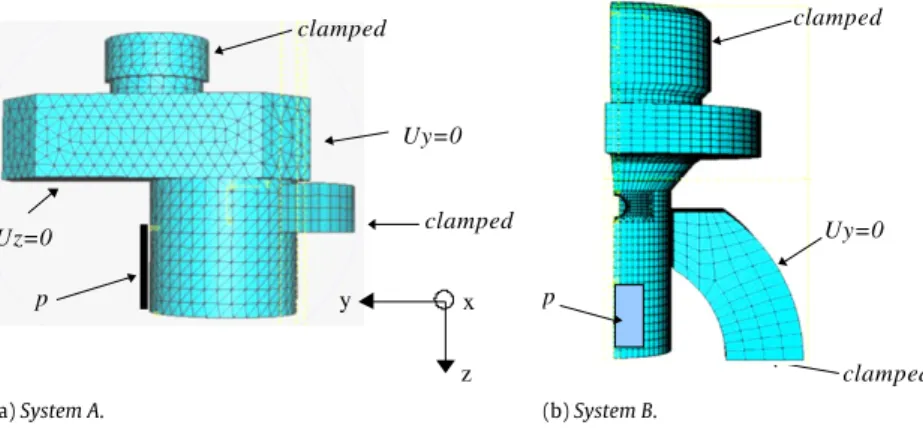
meshes and boundary conditions for system A and system B are shown inFig. 7. A second-order hexahedric 3D finite element with reduced integration
(
C 3D20R)
is employed except for system A where a modified 3D tetrahedric finite element(
C 3D10M)
is used. In these models, the material properties are fixed to their minimal values with a weak probability of obtaining these values. So, the present models are pessimist from this point of view, which goes in the direction of safety.3.3. Response surface
Following the initial aim, a Response Surface (RS) is now elaborated in order to easily assess UA
=
UA(
dfr,
h,
p)
for any(
dfr,
h,
p)
set avoiding consuming time. Because of this surface(one for each system), it becomes convenient to evaluate the performance function in the next and final step.
A second-order polynomial is classically obtained for UAusing
a multi-linear regression method. It is expressed in the following form:
UA
=
a0+
a1x1+
a2x2+
a3x3+
a12x1x2+
a13x1x3+
a23x2x3+
a11x21+
a22x22+
a33x23 (3)where
(
x1,
x2,
x3)
, respectively, stand for physical parameters(
dfr,
h,
p)
and a=
(
a0,
a1,
a2,
a3,
a12,
a13,
a23,
a11,
a22,
a33)
areestimated coefficients issued from a
=
(
xtx)
−1xty formula, where y stands for UAand x is the matrix of experiments.Uy=0 clamped clamped Uz=0 p y z x cl d clamped Uy=0 ampe p
(a) System A. (b) System B.
Fig. 7. Meshes and boundary conditions for system A and system B.
Fig. 8. Interpretation of the response surface for system A.
Involving more than two variables, the present surface is a hypersurface, not representable in the dimensions! Nevertheless, this hypersurface can be illustrated by fixing one of the three parameters.
Thus,Fig. 8gives a sketch of the RS in the case of system A. In each plot, the third free parameter is fixed to its mean value while the two other ones vary.
Estimating the quality of the previous response surface is essential to ensure that the physical phenomenon is correctly modelled. The gap between the FE calculations and RS prediction is first evaluated for 13
(
dfr,
h,
p)
initial set values. Second, 10additional FES are carried out using
(
dfr,
h,
p)
set values chosen inthe feasible design space to check the RS accuracy. These new FE results are compared with the RS predictions. In the case of large disagreement (relative variation higher than 10% not acceptable), a new response surface is elaborated including these new FES. It will be particularly important to evaluate the response surface quality at the
(
dfr,
h,
p)
set corresponding to the higher failure probability. 3.4. Reliability analysisThis final stage consists in evaluating the failure probability for the feared event traduced by Eq.(1). Using the RS is an efficient way to easily estimate the performance function G and see if the feared event is encountered or not. The use of the Monte Carlo method is now possible and the results can be considered as a reference provided that the number of trials is correctly linked to the probability level. Indeed, it needs around 10n+2to 10n+3trials
to evaluate a failure probability level of 10−n.
Approximated FORM and SORM methods are investigated in this work and compared with Monte Carlo and derivated Monte Carlo methods. An overview of these methods is now presented.
3.4.1. Monte Carlo (MC) method
In the Monte Carlo approach [12], all the variables are randomly sampled according to their statistical distribution. For each trial (a
set of data) the G function is calculated using the RS, Eqs.(1)and(3). Finally, the number of situations giving G negative is counted to ob-tain an estimation of the failure probability Pfin a simple way [13]:
˜
Pf=
1 N NX
r=1 IDfr (4)where N is the total number of trials, r is the current trial number and Ir
Dfthe counter of feared event realization. Using this method,
an error depending on the trials number and the estimated prob-ability level can advantageously be obtained by the Shooman for-mula [14] for a degree of confidence of 95%:
%erro
=
200s
1
− ˜
Pf N· ˜
Pf.
(5)This method, illustrated inFig. 9in standard space [13], can be very time consuming when the limit state function calculation is complex and needs experiments or FE calculations, as explained above.
Nevertheless, it becomes efficient when an analytical expres-sion of this function can be established using the response surface, as in the present study.
3.4.2. FORM/SORM approximated methods
FORM and SORM methods consist in an analytical approxima-tion of the failure probability by calculating a reliability index,
β
[13]. It is necessary in this case to formulate the limit state, Eq.(1), in a reduced variable space (standard space) where each variable has a zero mean and unit standard deviation. The transformation for a given Gaussian distribution from physical space, xivariables,to standard space, uivariables, is called an isoprobabilistic
trans-formation and is expressed
ui
=
xi−
miσ
i(6)
0 2 -2 4 Safe.domain 6 8 10 0 1 2 3 4 5 -2 -1
Fig. 9. Classical Monte Carlo method illustrated in standard space.
In the previous standard space, the reliability index
β
represents the shortest distance from the limit state surface to the origin; seeFig. 9. P∗defines the most probable point of failure.Optimisation algorithms are then needed to determine the
β
index. Genetic algorithms are investigated for this purpose, looking for the best value of this index (global minimum) [15,16].Then, knowing the index
β
, the failure probability can be easily determined using the standard normal Cumulative Distribution Function (CDF)ϕ
.For instance, for the FORM method, where the limit state is approximated by a first-order hyperplane, it is expressed by
Pf
=
φ(−β) =
1−
φ(β).
(7)In the case of the SORM approach, where the limit state is approximated by a second-order hypersurface, it is given by the Breitung formula [17]: Pf
=
φ(−β)
*
n−1Y
j=1 1p
(
1+
β
kj)
+
(8)where the coefficients kj permit one to take into account the
curvature of the limit state [13] at P∗.
Thus, the failure probability calculation can be suitable provided that
β
obtained from the optimization algorithms is sufficiently accurate: its determination is of first importance.Using deterministic optimization algorithms [18–20], the xi
variables corresponding to P∗can be obtained. From these values,
sensitivities and elasticities useful for design, Eq. (11), can be estimated.
Moreover, in a particular condition where only two indepen-dent Gaussian variables, R and S, are considered,
β
can be obtained analytically byβ =
q
R¯
− ¯
S(σ
2R
+
σ
S2)
(9)
whereR and
¯
S denote the mean of R and S respectively, and¯
σ
Randσ
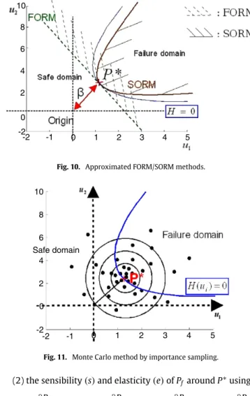
Srepresent the standard deviation of R and S respectively.With the FORM or SORM method, illustrated inFig. 10, no error estimation is available, in contrast to the Monte Carlo approach.
In addition to obtaining the critical set values of variables (P∗, not achievable using the Monte Carlo method), significant
information can be also assessed by FORM/SORM methods: (1) the influence of each variable near the critical set values using
α
icoefficients defined byα
i=
∂β
∂
ui;
and (10) 0 2 -2 4 6 8 10 0 1 2 3 4 5 -2 -1Fig. 10. Approximated FORM/SORM methods.
0 -2 -2 -1 2 4 6 8 10 0 1 2 3 4 5 Safe domain
Fig. 11. Monte Carlo method by importance sampling.
(2) the sensibility
(
s)
and elasticity(
e)
of Pf around P∗using e1i=
mi Pf∂
Pf∂
mi;
e2i=
σ
i Pf∂
Pf∂σ
i;
S1i=
∂
Pf∂
mi;
S2i=
∂
Pf∂σ
i.
(11) As presented below, FORM/SORM and Monte Carlo methods may be combined in derivated Monte Carlo methods.3.4.3. Derivated Monte Carlo method (DMC): Monte Carlo by importance sampling
This method, presented in [13], is also used in this work. Knowing P∗, it consists in concentrating sampling around this
point determined before. An illustration of this method is given in Fig. 11. So, if no other secondary local minima exist, the probability of failure can be assessed using Eq.(12)with a minimum number of trials. With this method, only a few thousands of trials are enough to obtain a probability of 10−7instead of 109using the classical Monte Carlo method.
˜
Pf=
1 N NX
A=1 IDfr expX
i u∗i·
uri−
β
2!
(12) where u∗ i represent the P∗co-ordinates in standard space, ur i the
co-ordinates of variable i for trial r, Ir
Df the number of failures and N the number of trials.
Nevertheless, the quality of results using Monte Carlo simula-tions is highly dependent on the quality of the generator of pseudo-random numbers. The ‘Mersenne Twister’ generator, developed by Matsumoto and Nishimura [21], is implemented in the reliability tool used for this study [1].
1 1 0 2 2 3 3 -3 -2 -1 0 -3 -2 -1
Fig. 12. Convex limit state.
Table 3
Distributions of system A variables. Variable Unit Distribution Mean
value Standard deviation Minimum value Maximum value ds mm tr. Gaussian 2.072 0.037 1.937 2.207 dfi mm tr. Gaussian 0.469 0.037 0.335 0.60 dfr mm tr. Gaussian 0.159 0.044 0.0 0.318 h mm tr. Gaussian 3.824 0.06 3.689 3.959 p MPa uniform 100 80 120
4. Results and discussions
4.1. Concerning reliability tools
Before applying them for present complex system A and system
B, the relevance of previous reliability tools has been first evaluated
on reference tests obtained from the literature [22–26]. Many nonlinear performance functions have been involved in those tests. Considering the quadratic limit state function, see Fig. 12, it appears obvious that FORM/SORM methods must be used very carefully. As demonstrated earlier [25], such cases can lead to significant overestimation or underestimation of the failure probability.
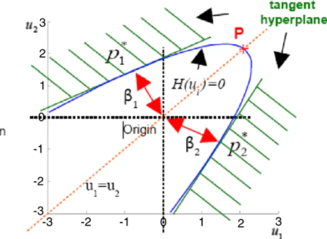
Moreover, if several critical points P1∗and P2∗that are physically acceptable exist, genetic algorithms can be advantageously used while deterministic algorithms should converge to point P, which is not the critical one. In such a case where several convenient critical points exist, a multi-FORM approach [13] is clearly recommended to correctly evaluate the failure probability level.
4.2. Concerning system A and system B reliability 4.2.1. System A
The ds
,
dfi,
dfr,
h and p distributions are given inTable 3, wherethe truncated Gaussian distribution is denoted by tr. Gaussian. Several optimization calculations using the Abdo–Rackwitz [18], BFGS [19] or SQP [20] deterministic algorithms have been per-formed changing the initial starting point. Scanning all over the design space, only one critical point has been found every time. The reliability index,
β
, the failure probability, Pf, and the criticaldesign point obtained from FORM, SORM and DMC methods are summarized inTable 4. DMC needs 3
×
105simulations whereas FORM and SORM need only 365.Table 4
Characteristics of critical design point.
β Critical design point Failure probability
5.78 p dfr h dfi dS FORM:Pf=3.72×10⁻⁹ 119.773 0.249 3.700 0.575 1.965 SORM:Pf=6.02×10⁻¹⁰ Monte Carlo: 4.53×10⁻¹⁰ 500 400 300 200 100 0 -100 -200
Fig. 13. Elasticity diagram concerning system A.
Obtaining the critical design point, it is necessary to verify the quality of the response surface at this point.
So, a new FE simulation with ds
,
dfi,
dfr,
h and p correspondingto the critical point is performed to obtain UAFEand compare this value to URS
A obtained by the RS. A variation of 2.5 % is obtained
in this case. This result is acceptable as regards the system safety since UAis overestimated by the response surface.
Table 4 reveals a gap between the FORM and SORM results. This can be explained by the nonlinear limit state around the critical point. Moreover, the gap between SORM and Monte Carlo results probably means that the SORM is not sufficient to cover the nonlinearity around the critical point.
Moreover, approximated FORM and SORM methods can advantageously give information about the Pf sensibility to the
mean value [MEA], standard deviation [SD], minimum value [MIN] and maximum value [MAX ] of each variable. Such information is contained in the elasticity diagram presentedFig. 13.
Obviously, Pf is very sensitive to pressure p[max]: Pf goes up by
500% when the p[max]value goes up 1%. The pressure needs to be
controlled very carefully. In contrast, Pfis logically reduced by an
increase of dsand h mean values. Finally, Pf is not sensitive to the
standard deviation of each parameter except for pressure. So, it will be slightly affected by a bad quality control during manufacturing.
Table 5
Distributions of system B variables. Variable Unit Distribution Mean
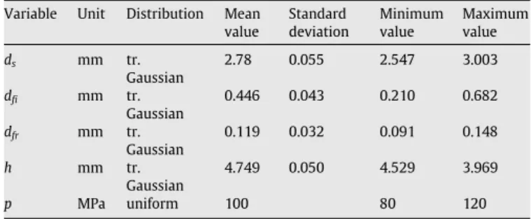
value Standard deviation Minimum value Maximum value ds mm tr. Gaussian 2.78 0.055 2.547 3.003 dfi mm tr. Gaussian 0.446 0.043 0.210 0.682 dfr mm tr. Gaussian 0.119 0.032 0.091 0.148 h mm tr. Gaussian 4.749 0.050 4.529 3.969 p MPa uniform 100 80 120 Table 6
Critical design point and failure probability for system B.
β Critical design point Failure probability
2.89 p dfr h dfi dS FORM:Pf=1.90×10⁻³ 119.476 0.118 4.703 0.488 2.706 SORM:Pf=6.50×10⁻⁴ Monte Carlo: 6.45×10⁻⁴ -50 -100 250 200 150 100 50 0
Fig. 14. Elasticity diagram concerning system B.
In spite of the pessimist FE model and a response surface overestimating this model, Pf is less than 10−9, which is very far
from 10−4required, so the system seems to be largely secure!
4.2.2. System B
For this system, the ds
,
dfi,
dfr,
h and p distributions are given inTable 5and the results are summarized inTable 6.
The SORM result is very close to Monte Carlo one using approximately 6
×
105 trials, but this indicates that thespecification is just satisfied.
Moreover, an FE simulation with ds
,
dfi,
dfr,
h,
p correspondingto the critical point leads to a relative error of 6.5%. In this case, the displacement UAissued from response surface is underestimated.
So, the failure probability is also underestimated, which is not acceptable.
Improvements must be done on this system to ensure the specification. The elasticity diagram plotted in Fig. 14 is very useful to point out ways of improvements. It indicates that the failure probability level is largely influenced by the pressure p and distance h. It can also be observed that the failure probability level is not sensitive to the standard deviation of each parameter.
4.3. Ways of improvements for system B
Two ways of improvement are suggested byFig. 14.
First, a better knowledge of p distribution would probably permit one to reduce the failure probability level. For instance, if the maximum value of p is 118 MPa rather than 120 MPa, then Pf
becomes 2
.
69×
10−6instead of 6.
45×
10−4! In the same way, if pFig. 15. System B configuration.
follows a truncated Gaussian distribution with 100 MPa as its mean value, 50 MPa as the standard deviation, 80 MPa as minimum value and 120 MPa as maximum value instead of a uniform distribution,
Pfis 9
.
57×
10−7instead of 6.
45×
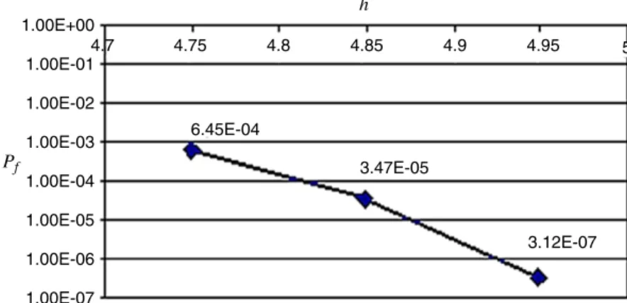
10−4!A second way of improvement consists in increasing the distance h and reducing the distance a; seeFig. 15. As shown in Fig. 16, this permits one to largely decrease the failure probability level. So, by reducing by 0.2 mm the distance a, Pf changes from
6
.
45×
10−4to 3.
12×
10−7.5. Conclusion
In this work, a reliability approach is developed for analysing the safety of locking systems. A mechanic–reliability engineer method, combining both mechanical and reliable tools, is proposed to assess the failure probability Pf of those systems including
un-certainties. Experimental Design (ED), Finite Element Simulations (FES), the Response Surface (RS) and Reliability Analysis (RA) com-pose the successive stage of the present methodology. It appears convenient to conclude this study with reference to three points:
(1) an engineer’s point of view about the reliability of system
A and system B underlining the analysis reliability engineer like
decision-making aid,
(2) an advised user’s point of view about the use of modelisation and reliability tools,
(3) a researcher’s point of view concerning improvements in future works.
About the reliability of system A and system B.
The very great robustness of the first system of locking (system A) and the weak safety margin for system B have been demonstrated. Improvements of system B have been possible from the analysis of the diagram of elasticities. This revealed that the level of failure probability was significantly affected by the distribution of the pressure. A better knowledge of this distribution would probably lead to a level of probability of weaker failure. Moreover, the second way of improvements proposed (modification of the a and h dimensions) also showed that the mechanic–reliability engineer method could be advantageously used as a decision-making aid method.
About modelisation and reliability tools.
A suitable ED has been used to elaborate a second-order polynomial as the RS. Necessary data to identify this second-order polynomial have been obtained by FES. At this stage, the capacity of the model to correctly represent the physical phenomenon only depends on the quality of the RS. Robust indicators are necessary to estimate this quality. Using a reliable RS, it is now possible to perform a reliability analysis using appropriate tools. The investigations made in this study showed it was convenient to use FORM and SORM methods in addition to the Monte Carlo method.
1.00E+00 4.7 4.75 6.45E-04 3.47E-05 3.12E-07 4.8 4.85 h Pf 4.9 4.95 5 1.00E-01 1.00E-02 1.00E-03 1.00E-04 1.00E-05 1.00E-06 1.00E-07
Fig. 16. Evolution of the failure probability on increasing h; System B configuration.
About future works.
In this paper, no effort was made to improve the distributions of the variables. We will concentrate on this particular point in future works. Investigations will relate precisely to the means of improving the distributions of sensitive variable at the design point while carrying out a minimum of tests.
References
[1] Phimeca software. Software for reliability analysis developed by Phimeca Engineering S.A.
[2] Abaqus/standard user’s manual. vol. I.
[3] Sang-Min L, et al. Failure probability assessment of wall-thinned nuclear pipes using probabilistic fracture mechanics. Nuclear Engineering and Design 2006; 236(4):350–8.
[4] Sudret B, Guédé Z. Probabilistic assessment of thermal fatigue in nuclear components. Nuclear Engineering and Design 2005;235(17–19):1819–35. [5] Mohamed AM, Lemaire M. Linearized mechanical model to evaluate reliability
of offshore structures. Structural Safety 1995;17(3):167–93.
[6] Melchers RE. The effect of corrosion on the structural reliability of steel offshore structures. Corrosion Science 2005;47(10):2391–410.
[7] Schotanus MIJ, et al. Seismic fragility analysis of 3d structure. Structural Safety 2004;26(4):421–41.
[8] Kim S-H, Na S-W. Response surface method using vector projected sampling point. Structural Safety 1997;19(1):3–19.
[9] Gupta S, Manohar CS. An improved response surface method for the determination of failure probability and importance measures. Structural Safety 2004;26:123–39.
[10] Gayton N, Bourinet JM, Lemaire M. CQ2RS: A new statistical approach to the response surface method for reliability analysis. Structural Safety 2003;25(1): 99–121.
[11] Box GEP, Hunter JS. Statistics for experimenters. New York (NY): John Wiley & Sons; 1978.
[12] Rubinstein RY. Simulation and the Monte Carlo methods. John Wiley and Sons; 1981.
[13] Lemaire M. Fiabilité des structures, couplage mécano-fiabiliste statique. In: Hermes science. Lavoisier; 2005.
[14] Shooman ML. Probabilistic reliability: An engineering approach. New York (NY): Mc Graw Hill Book Co.; 1968.
[15] Goldberg DE, Paz EC. Efficient parallel genetic algorithms: Theory and practice. Computer Methods in Applied Mechanics and Engineering 2000;186: 221–238.
[16] Maeda Y, Ishita M, Li Q. Fuzzy adaptative search method for parallel genetic algorithm with island combination. International Journal of Approximate Reasoning 2006;41:59–73.
[17] Breitung K. Asymptotic approximation for multinormal integrals. Journal of Engineering Mechanics Division, ASCE 1984;110(3):357–66.
[18] Abdo T, Rackwitz R. A new beta-point algorithm for large time-invariant and time variant reliability problems. In: Reliability and optimization of structures. In: 3th WG 7.5 IFIP conference. 1990. p. 1–11.
[19] Fletcher R, Powel MJD. A rapidly convergent descent method for minimization. Computer Journal 1963;6:163–8.
[20] Papalambros PY, Wilde DJ. Principles of optimal design. NY (USA): Cambridge University Press; 1988.
[21] Matsumoto M, Nishimura T. Mersenne twister: A 623-dimensionally equidis-tributed uniform pseudorandom number generator. ACM Transactions on Modeling and Computer Simulation 1998;8(1):3–30.
[22] Borri A, Speranzini E. Structural reliability analysis using a deterministic finite element code. Structural Safety 1997;19(4):361–82.
[23] Kim S-H, Na S-W. Response surface method using vector projected sampling point. Structural Safety 1997;19(1):3–19.
[24] Gayton N, Bourinet JM, Lemaire M. CQ2RS: A new statistical approach to the response surface method for reliability analysis. Structural safety 2003;25(1): 99–121.
[25] Elegbede C. Structural reliability assessment based on particles swarm optimization. Structural Safety 2005;27:171–86.
[26] Der Kiureghian A, Haukaas T, Fujimura K. Structural reliability software at the University of California, Berkeley. Structural Safety 2006;28:44–67.