To cite this version :
Alexandr KLIMCHIK, Anatol PASHKEVICH, Sébastien GARNIER, Stéphane CARO, François LEONARD, Gabriel ABBA, Jinna QIN - Simulation results using a robot with flexibilities for machining and welding - 2014
Projet COROUSSO Livrable n°4.3 Résultats en simulations de l’utilisation d’un robot avec flexibilités pour l’usinage et le soudage ANR‐10‐SEGI‐003‐LI 4.3 15/09/2014 indice A Page de garde
C
orousso
Projet COROUSSO
ANR‐10‐SEGI‐003
Tâche 4 : Commande du système procédé‐robot
Livrable 4.3 : Résultats en simulation de
l’utilisation d’un robot avec flexibilités pour
l’usinage et le soudage
Projet ANR‐2010‐SEGI‐003‐COROUSSO
Partenaires :
P Sig In r Nom BOUJDAINE PASHKEVICH LEONARD Fr Date Nom(s) gnature(s) ndice de révision M Fatiha Anatol rançois Rédi 1/07 A. KLIMCH A. PASHKEV S. GARNI S. CARO F. LEONA G. ABB J. QIN Modifié par igé par 7/2014 HIK – IRCCyN VITCH‐IRCCyN IER‐IRCCyN O‐IRCCyN ARD – LCFC BA – LCFC N – LCFC Descrip List Orga AN HA EM EN N ption des pri te de diffusio nisme NR AL MN NIM Approuvé 30/09/20 G. ABBA – incipales évo on par 014 LCFC olutions G Date de mis applicatio Fonction PR MCF Validé par 30/09/201 G. ABBA – LC se en on co n r 4 CFC Pages oncernées
C
oro
1
Intro
2
Modè
2.1 M 2.2 M2.2.1
2.2.2
2.3 E 2.4 M 2.5 M3
Résul
3.1 E 3.2 E4
Résul
4.1 V5
Conc
6
Biblio
Les a pour la rédausso
duction ...
èles de simu
Modèle simp Modèle avecModèle
Modèle
Environneme Modèle du pr Modèle du prltats de sim
Exemples av Exemple aveltats de sim
Validation delusion ...
ographie ...
uteurs s’exc action de ce R d’un...
ulation ...
plifié du com raideurs loce de flexibil
e de flexibil
ent de simula rocédé d’usin rocédé FSWmulation en
ec un modèl ec un modèlemulation po
es compensa...
...
usent par av rapport. Pro L ésultats en s n robot avecSO
...
...
mportement fl calisées ...lités dans l’
lités dans l’
ation ... nage ... ...usinage ....
e d’usinage « e d’usinage àour le procé
ateurs en simu...
...
vance auprès ojet COROUS Livrable n°4.3 simulations d flexibilités p le soudageOMMA
...
...
lexible du rob ...espace cart
espace artic
... ... ......
« Grid based à effort spécifédé FSW ...
ulation ......
...
s du lecteur SSO 3 de l’utilisatio pour l’usinagAIRE
...
...
bot ... ...ésien ...
culaire ...
... ... ......
d Model » ... fique de coup...
......
...
de l’utilisatio on e et A...
...
... ......
...
... ... ......
... pe ......
......
...
on de deux l ANR‐10‐SEGI‐ 15/09/2 indice Page 3 Au A.P G.A...
...
... ......
...
... ... ......
... ......
......
...
langues (fran ‐003‐LI 4.3 2014 e A 3/34 uteurs : A P, S.G, S.C, F A, J.Q...
...
... ......
...
... ... ......
... ......
......
...
nçais et angl A.K, F.L,... 5
... 6
... 6 ... 6... 6
. 10
. 12 . 14 . 18. 20
. 20 . 27. 29
. 29. 31
. 32
ais)Projet COROUSSO Livrable n°4.3 Résultats en simulations de l’utilisation d’un robot avec flexibilités pour l’usinage et le soudage ANR‐10‐SEGI‐003‐LI 4.3 15/09/2014 indice A Page 5/34 Auteurs : A.K, A.P, S.G, S.C, F.L, G.A, J.Q
C
orousso
1 INTRODUCTION
L’objectif de cette tâche est de détailler les modèles utilisés en simulation et les résultats obtenus en simulation aussi bien pour le procédé d’usinage que pour le procédé FSW. De cette manière, on peut se rendre compte du comportement du robot durant le procédé et ainsi prévoir les meilleurs réglages mais également de limiter les coûts des essais qui seront réalisés dans la tâche 5.
Ce livrable contient donc dans une première partie les détails sur la modélisation des flexibilités des robots essentiellement par le biais d’un modèle de flexibilités localisées. Les flexibilités sont exprimées aussi bien dans l’espace cartésien des robots que dans l’espace articulaire et en tenant compte des éventuels couplages.
Une seconde partie traite du modèle dynamique utilisé dans le simulateur et de l’environnement de simulation. Un travail non négligeable a été de modéliser également le contrôleur de robot de l’entreprise Kuka.
Les procédés d’usinage et de soudage FSW sont eux‐mêmes modélisés par des modèles simples mais traduisant bien la réalité du comportement. Ces modèles sont issus des livrables 2.1 à 2.3 et du livrable 3.4.
Ce rapport se termine par des résultats obtenus en simulation en usinage d’une part avec un robot Kuka KR 270 à l’Iut de Nantes et d’autre part en soudage FSW avec un robot Kuka KR 500 MT2 à l’institut de Soudure de Goin.
2 MODÈLES DE SIMULATION
2.1 Modèle simplifié du comportement flexible du robot
The dynamic behaviour of the robot under the loading F caused by technological process can be described as
M δt C δt K δt FC &&+ C &+ C = (1)
where M is 6 6C × mass matrix that represents the global behaviour of the robot in terms of natural
frequencies, C is 6 6C × damping matrix, K is 6 6C × Cartesian stiffness matrix of the robot under the
external loading F , δt δt& and δt&& are dynamic displacement, velocity and acceleration of the tool end‐point , in a current moment respectively (Briot, 2011).
In general, the cutting force Fc has a nonlinear nature and depends on many factors such as cutting conditions,
properties of workpiece material and tool cutting part, etc. (Ritou, 2006). But, for given tool/workpiece combination, the force Fc could be approximated as a function of an uncut chip thickness h, which represents
the desired thickness to cut at each instant of machining.
Hence, to reduce errors caused by cutting forces in the robotic‐based machining it is required to obtain an accurate elasto‐static model of robot and elasto‐dynamic model of machining process. These problems are addressed in the following sections taking into account some particularities of the considered application (robotic‐based milling).
2.2 Modèle avec raideurs localisées
2.2.1 Modèle de flexibilités dans l’espace cartésien
Elasto‐static model. Elasto‐static model of a serial robot is usually defined by its Cartesian stiffness matrix,
which should be computed in the neighborhood of loaded configuration. Let us propose numerical technique for computing static equilibrium configuration for a general type of serial manipulator. Such manipulator may be approximated as a set of rigid links and virtual joints, which take into account elasto‐static properties (Figure 1). Since the link weight of serial robots is not negligible, it is reasonable to decompose it into two parts (based on the link mass centre) and apply them to the both ends of the link. All this loadings will be aggregated in a vector G=
[
G G , where 1... n]
G is the loading applied to the i‐th node‐point. Besides, it is assumed that i the external loading F (caused by the interaction of the tool and the workpiece) is applied to the robot end‐ effector.Projet COROUSSO Livrable n°4.3 Résultats en simulations de l’utilisation d’un robot avec flexibilités pour l’usinage et le soudage ANR‐10‐SEGI‐003‐LI 4.3 15/09/2014 indice A Page 7/34 Auteurs : A.K, A.P, S.G, S.C, F.L, G.A, J.Q
C
orousso
Figure 1 : VJM model of industrial robot with end-point and auxiliary loading
Following the principle of virtual work, the work of external forces ,G F is equal to the work of internal forces θ τ caused by displacement of the virtual springs δθ
(
T)
T θT 1 δ δ δ n j j j= ⋅ + ⋅ = ⋅∑
G t F t τ θ (2)where the virtual displacements δt can be computed from the linearized geometrical model derived from j
( ) θ δ jδ , 1.. j= j= n t J θ , which includes the Jacobian matrices ( )θ
( )
, j j = ∂ ∂ J g q θ θ with respect to the virtual joint coordinates. So, expression (2) can be rewritten as(
T ( )θ) (
T ( )θ)
θT 1 δ δ δ n j n j j= ⋅ ⋅ + ⋅ ⋅ = ⋅∑
G J θ F J θ τ θ (3)which has to be satisfied for any variation of δθ . It means that the terms regrouping the variables δθ have the coefficients equal to zero. Hence the force balance equations can be written as θ θ( )T ( )Tθ 1 n j n j j= =
∑
⋅ + ⋅ τ J G J F (4) These equations can be re‐written in block‐matrix form as τθ =Jθ(G)T⋅ +G J(F)Tθ ⋅F (5) where J(F)θ =J , ( )θn (G) (1) ( ) θ θ θ T T... nT ⎡ ⎤ = ⎣ ⎦J J J , G= ⎣⎡G1T...GnT⎦⎤T. Finally, taking into account the virtual spring reaction τθ=K θ , where θ⋅ Kθ=diag
(
Kθ1,...,Kθn)
, the desired static equilibrium equations can bepresented as
Jθ(G)T⋅ +G J(F)Tθ ⋅ =F K θ θ⋅ (6)
To obtain a relation between the external loading F and internal coordinates of the kinematic chain θ corresponding to the static equilibrium, equations (6) should be solved either for different given values of F or for different given values of t . Let us solve the static equilibrium equations with respect to the manipulator configuration θ and the external loading F for given end‐effector position t g θ and the function of =
( )
auxiliary‐loadings G θ
( )
K θ Jθ⋅ = θ(G)TG J+ (F)Tθ F t g θ; =
( )
; G G θ =( )
(7) where the unknown variables are( )
θ F . ,kinematic equations may be linearized in the neighbourhood of the current configuration θ i
ti+1=g θ
( )
i +Jθ(F)( ) (
θi ⋅ θi+1−θi)
; (8)where the subscript 'i' indicates the iteration number and the changes in Jacobians J(G)θ ,J and the auxiliary (F)θ loadings G are assumed to be negligible from iteration to iteration. Correspondingly, the static equilibrium equations in the neighborhood of θ may be rewritten as i Jθ(G)T⋅ +G J(F)Tθ ⋅Fi+1=K θ . θ⋅ i+1 (9) Thus, combining (8), (9) and analytical expression for θ 1( (G)Tθ (F)Tθ ) − = ⋅ + ⋅ θ K J G J F , the unknown variables F and θ can be computed using following iterative scheme
(
)
(
( )
)
(
)
1 (F) 1 (F)T (F) (F) 1 (G)T θ θ θ θ θ 1 (G)T (F)T θ θ θ 1 1 1 1 i i i i i i i i θ θ − − − − + + + + = ⋅ ⋅ − + − = ⋅ + ⋅ F J K J t g θ J θ J K J G θ K J G J F (10) The proposed algorithm allows us to compute the static equilibrium configuration for the serial robot under external loadings applied to any point of the manipulator and the loading from the technological process. Stiffness matrix. In order to obtain the Cartesian stiffness matrix, let us linearize the force‐deflection relationin the neighborhood of the equilibrium. Following this approach, two equilibriums that correspond to the manipulator state variables ( , , )F θ t and (F+δ ,F θ+δ ,θ t+δ )t should be considered simultaneously. Here,
notations δF , δt define small increments of the external loading and relevant displacement of the end‐point. Finally, the static equilibrium equations may be written as t g θ=
( )
; K θ Jθ⋅ = θ(G)T⋅ +G J(F)Tθ ⋅F (11) and(
)
(
)
(
(G) (G))
T(
)
(
(F) (F))
T(
)
θ θ θ θ θ δ δ δ δ δ δ δ + = + ⋅ + = + ⋅ + + + ⋅ + t t g θ θ K θ θ J J G G J J F F (12) where t F G K θ are assumed to be known. , , , θ, After linearization of the function ( )g θ in the neighbourhood of the loaded equilibrium, the system (11), (12) is reduced to equations (F) θ (G) (G) (F) (F) θ θ θ θ θ δ δ δ δ δ δ δ = ⋅ = + + + t J θ K θ J G J G J F J F (13)which defines the desired linear relations between δt and δF . In this system, small variations of Jacobians may be expressed via the second order derivatives δJ(F)θ =Hθθ(F)⋅δθ , δJ(G)θ =H(G)θθ ⋅δθ , where
Projet COROUSSO Livrable n°4.3 Résultats en simulations de l’utilisation d’un robot avec flexibilités pour l’usinage et le soudage ANR‐10‐SEGI‐003‐LI 4.3 15/09/2014 indice A Page 9/34 Auteurs : A.K, A.P, S.G, S.C, F.L, G.A, J.Q
C
orousso
(G) 2 θθ 1 2 T j j j n = =
∑
∂ ∂ H g G θ , (F θθ 2 )= ∂2 T ∂H g F θ . Also, the auxiliary loading G may be computed via the first
order derivatives as δG= ∂G θ θ ∂ ⋅δ
Further, let us introduce additional notation Hθθ=Hθθ(F)+Hθθ(G) +J(G)Tθ ⋅∂ ∂G θ , which allows us to present system (13) in the form (F) θ (F)T θ θ θθ δ δ δ ⎡ ⎤ ⎡ ⎤= ⋅⎡ ⎤ ⎢ ⎥ ⎢ ⎥ − + ⎢ ⎥ ⎣ ⎦ ⎣ ⎦ ⎣ ⎦ 0 J t F 0 J K H θ (14) So, the desired Cartesian stiffness matrices K can be computed as C KC =
(
Jθ(F)(Kθ−Hθθ)−1Jθ(F)T)
−1 (15) Below, this expression will be used for computing of the elasto‐static deflections of the robotic manipulator.Mass matrix. To evaluate dynamic behaviour of the robot under the loading, in addition to the Cartesian
stiffness matrix K it is required to define the mass matrix C M . Comprehensive analysis and definition of this C
matrix have been proposed in (Briot, 2011). Here, let us summarise the main results that will be used further in the error compensation technique.
Similar to the stiffness matrix, here physical properties defined by the mass matrix M are constant in the C
joint coordinates Mθ =const and are defined by the mass matrices M of all n links of the robot θi θ=diag( θ1,..., θn)
M M M . Assuming that link may be approximated by a beam with a constant cross‐section,
the mass matrix M can be computed as θi
Mθi=diag a a a a a a( ,1 2, 3, 4, 5, 6) (16)
where a1=mi/ 3, a2=33mi/ 140, a3=33mi / 140, 4 / 3
p i i i
a =I ρL , a5=8Iiyρi iL /15, a6=8Iizρi iL / 15, m is i
physical mass of i‐th link, ρi is density of i‐th link, L is link length, i p i
I is the polar moment, y, z
i i
I I are the
second moments of the area. Since the mass matrix M is defined in the joint coordinates it can be θ
recomputed into the Cartesian coordinates associated with the tool end‐point using the Jacobian matrix J θ
(which depend on the robot configuration q and computed with respect to virtual joint coordinates θ ) using following expression
MC=J M J θT θ θ (17)
Thus, using expressions (16) and (17) it is possible to compute the mass matrix M for a given robot C
La flexibilité des robots est souvent bien analysée sur les robots légers, par exemple, le Kuka‐DLR LWR, le Barrett WAM, le Bras ASSIST, etc. Les robots manipulateurs lourds comme les robots utilisés dans cette étude sont souvent considérés comme rigides. Mais pour une opération qui demande des efforts très importants, la déformation à cause de la flexibilité ne peut pas être négligée, si l’on désire obtenir de bonnes performances de fabrication. De nombreuses recherches ont été faites sur la modélisation des robots. Les modèles les plus souvent utilisés pour les robots manipulateurs sont décrits dans les ouvrages (Craig et al., 1986), (Sciavicco and Siciliano, 2000) et (Spong et al., 2005). Les principes fondamentaux et les méthodes qui sont utilisées pour modéliser, concevoir et piloter un système robotique ainsi que la planification et la commande d’un robot réel sont discutés dans (Siciliano and Khatib, 2008).
La première étude des problèmes liés à la présence de transmissions flexibles dans les robots manipulateurs remonte à (Sweet and Good, 1985), (Good et al., 1985), avec les premiers résultats expérimentaux sur le bras GE P‐50. Des considérations mécaniques impliquées dans la conception des bras robotiques et dans l’évaluation de leurs éléments peuvent être trouvées dans (Rivin, 1988). Une analyse bibliographique sur la dynamique des manipulateurs flexibles peut être trouvée dans (Dwivedy and Eberhard, 2006). Du point de vue de la modélisation des manipulateurs flexibles, on peut supposer que la flexibilité est localisée au niveau des articulations et/ou distribuée le long des corps. En effet, ces deux types de flexibilité peuvent être présents en même temps. Les flexibilités aux articulations sont souvent présentées sur des robots industriels lorsque certains éléments de transmission de mouvement/réduction sont utilisés : les courroies, les longues tiges, les câbles, les réducteurs harmonic drive ou les trains d’engrenages épicycloïdaux. Ces composants permettent de placer les actionneurs au plus près de la base du robot, d’améliorer l’efficacité dynamique, ou de garantir des taux de réduction élevés. Par contre, sous des contraintes de forces importantes, ces composants deviennent intrinsèquement flexibles (Siciliano and Khatib, 2008).
Le modèle à articulations flexibles suppose que les élasticités sont concentrées dans la chaine de transmission mécanique entre les moteurs et les corps rigides du robot (Makarov, 2013). Les robots étudiés ici sont des robots séries à chaines ouvertes. Ces robots peuvent être considérés avec des articulations flexibles et une chaine cinématique ouverte à n + 1 corps rigides. La base et les n corps sont reliés par n articulations et actionnés par n moteurs électriques. De plus, toutes les articulations sont considérées comme flexibles (Siciliano and Khatib, 2008). De Luca a présenté en détail la modélisation de robots avec des éléments flexibles dans (De Luca and Book, 2008). Une étude sur les sources de flexibilités des robots séries a été faite par Dumas (Dumas, 2011). Les résultats montrent que les flexibilités localisées aux articulations sont les sources principales des flexibilités des robots séries. Quand il y a des réducteurs, on peut placer la déformation avant ou après le réducteur. L’élasticité au niveau de la transmission peut être modélisée par un ressort avec une raideur de torsion sur les axes de rotation et avec une raideur de traction/compression pour les axes en translation.
Les flexibilités localisées aux articulations peuvent s’expliquer aisément si on suppose qu’elles sont dues à la torsion de l’arbre de transmission des réducteurs. Si on adopte alors le modèle de la Figure 1, on obtient l’équation suivante :
C
oro
Avec Γ l’inverse de vecteur des Le mod Où : •J(q)
(6 •T
e= [
dans •Γm
=
•Γ = [Γ
• q = [ articu • θ = [θ des m • D(q)(6 et bo •I
a= d
•I = [I
1usso
Γ le vecteu e la matrice s angles artic dèle dynamiq 6×6) est la ma
[Fx Fy Fz Cx
le repère d’o[Γ
m1Γ
m2Γ
m3Γ
1Γ
2Γ
3Γ
4Γ
5 [q1 q2 q3 q4 ulaires, θ1 θ2 θ3 θ4 θ5 moteurs, 6×6) est la ma ornée,diag([I
a1I
a2I
1
I
2I
3I
4I
5I
6]
R d’un r des couple des rapport culaires. Figure 1 : que complet
q
D )
(
trice jacobiex Cy Cz]
T est outil (Rt) , 3Γ
m4Γ
m5Γ
m6Γ
6]
T est le v q5 q6]T, q&θ6]T,
θ
& etθ
&atrice d’inert
I
a3I
a4I
a5I
a6]
]
T est la matrPro L ésultats en s n robot avec
es à la sortie ts de réduct Flexibilité loc t du robot ut
q
H
q
&&
=
Γ
−
(
θ
&&
m aI
=
Γ
)
(
q
B
F
fr& =
)
(
q
B
F
fm& =
Γ enne du repè le torseur de 6]
T est le vec vecteur des c et q&& repréθ
&& représente tie généralisé T) est la mat
rice des cour ojet COROUS Livrable n°4.3 simulations d flexibilités p le soudagee des réduct ion des rédu
calisée sur l’ax tilisé dans le fr
q
F
q
q
,
&
)
−
(
T vF
N
Γ
−
−
(sig
F
q
B
s& +
s(si
F
q
B
m& +
m I kt m = Γ ère outil (Rt) es efforts ap cteur des co couples en so ésentent les ent les vecte ée du robot trice d’inerti rants moteur SSO 3 de l’utilisatio pour l’usinag teurs, K la ucteurs,θ
l xe de sortie d simulateur e Tq
T
J
q
&
)
−
(
)
)
(
θ
&
fmF
))
(q
gn &
))
(q
ign &
projeté dans pliqués sur l uples moteu ortie des réd s vecteurs d eurs des posi qui est sym e des arbres rs, on e et A matrice des le vecteur d des réducteurs est donc don eT
s le repère fix ’environnem rs, ducteurs, es positions tions, vitesse étrique, déf s moteurs, ANR‐10‐SEGI‐ 15/09/2 indice Page 11 Au A.P G.A s raideurs a es angles m rs nné par : xe (R0),. ment externe s, vitesses e es et accélér finie uniform ‐003‐LI 4.3 2014 e A 1/34 uteurs : A P, S.G, S.C, F A, J.Q rticulaires, N moteurs et q (1 (2 (2 (2 (2 e par le robot et accélératio rations des a mément posit A.K, F.L, v N q le 19) 20) 21) 22) 23) t ons xes tive) 1 6 ( x
&
compensation de gravité. Dans notre modèle, on tient donc également compte de l’effet du compensateur de gravité,
•
Bm
et Bs
: les matrices des coefficients de frottement visqueux au niveau des arbres moteurs et auxarticulations en Nm/[rad/s],
•
Fm
et Fs
: les matrices de frottement de Coulomb aux niveaux des moteurs des articulations en Nm,•
N
la matrice (6x6) des rapports de réduction et Nv son inverse.Tous les paramètres de ce modèle ont été identifiés (voir livrable 4.2, projet ANR Corousso) pour les robots Kuka KR270‐2F et KR500‐2MT.
Les valeurs des flexibilités (en Nm/rd) et des rapports de réduction sont données dans les tableaux ci‐ dessous.
K
ijK
1K
2K
3K
4K
5K
6KR270‐2F 3.8 ×10⁶ 6.6 ×10⁶ 3.9 ×10⁶ 5.6 ×10⁵ 6.6 ×10⁵ 4.7 ×10⁵ KR500 MT‐2 6.61 ×10⁶ 7.16 ×10⁶ 3.08 ×10⁶ ‐ ‐ ‐ Tableau 1 : Valeurs des raideurs articulaires des robots utilisés.
N
ijN
11N
22N
33N
44N
55N
66N
54N
64N
65KR270‐2F ‐219.00 ‐286.00 ‐ 270.177 ‐ 222.158 ‐ 221.765 157.552 1.002 2.020 2.520 KR500 MT‐ 2 469.375 469.375 ‐ 504.770 ‐ 260.619 ‐ 255.977 164.570 ‐1.0964 ‐1.5836 1.5311 Tableau 2 : Valeurs des coefficients de réduction des transmissions mécaniques des robots utilisés.
Ici,
est le vecteur des angles après réduction et avant la flexibilité des réducteurs. de
dimension 6
6 est la matrice des rapports de réduction. Elle est non diagonale à cause du couplage
entre axe 4, 5 et 6.
2.3 Environnement de simulation
Le simulateur a été développé dans un environnement de travail Matlab/Simulink©. Il est composé d’un fichier Simulink décrivant l’ensemble des équations de comportement du robot, du procédé et de la commande (y compris les capteurs et les boucles de retour en effort). La Figure 2 donne un exemple de la vue du simulateur et des différents blocs qui le composent.
C
orousso
R d’un Figur Pro L ésultats en s n robot avec re 2 : schéma ojet COROUS Livrable n°4.3 simulations d flexibilités p le soudage bloc du simu SSO 3 de l’utilisatio pour l’usinag lateur sous Si on e et A imulink© ANR‐10‐SEGI‐ 15/09/2 indice Page 13 Au A.P G.A ‐003‐LI 4.3 2014 e A 3/34 uteurs : A P, S.G, S.C, F A, J.Q A.K, F.L,
ce mémoire est donné ci‐dessous. Les blocs en bleu représentent la partie de la commande du robot, en rouge la régulation de force, en gris le générateur de trajectoire, en vert le système simulant le comportement dynamique des moteurs, et en orange la partie correspondant à la dynamique des axes du robot, ensuite en magenta la partie liée aux flexibilités, et en violet le modèle du procédé. Dans ce simulateur, les modèles du robot et du procédé peuvent être remplacés par ceux d’un autre robot ou procédé.
Les fonctions des blocs dans le simulateur sont :
• Générateur de trajectoire : transfert les trajectoires désirées Td =
(
pd vd ad)
(positions, vitesseset accélérations désirées, respectivement) du repère cartésien aux articulaires
(
q
dq
&
dq
&&
d)
; • P contrôleur : régulateur proportionnel d’asservissement de la position ; • PI contrôleur : régulateur proportionnel‐intégral d’asservissement de la vitesse ; • DNL : Dynamique Non‐Linéaire ; • Modèle Dynamique du Moteur : modèle dynamique des moteurs ; • Réducteurs : avec les rapports de transmission et intégral ; • Flexibilité : modèle de la flexibilité aux articulations ; • Modèle Dynamique du Robot : modèle dynamique du robot ; • Force Procédé : modèle d’effort du procédé ; • Régulateur de force : régulateur proportionnel‐intégral des efforts.2.4 Modèle du procédé d’usinage
Let us obtain the model of the cutting force which depends on the relative position of the tool with respect to the workpiece at each instant of machining. As follows from previous works (Brissaud, 2008), for the known chip thickness h, the cutting force Fc can be expresses as:( )
(
)
2 0 , 0 1 s s c s p h h r h h F h k a h h h + = ≥ + (24)where a is a depth of cut, p r k k= ∞ 0< depends on the parameters k1 ∞, k0 that define the so called stiffness of the cutting process for large and small chip thickness h respectively (Figure 3) and hs is a specific chip thickness, which depends on the current state of the tool cutting edge. The parameters k0, hs, r are evaluated experimentally for a given combination of tool/working material. To take into account the possible loss of contact between the tool and the workpiece, expression (24) should be supplement by the case of h< as 0
Projet COROUSSO Livrable n°4.3 Résultats en simulations de l’utilisation d’un robot avec flexibilités pour l’usinage et le soudage ANR‐10‐SEGI‐003‐LI 4.3 15/09/2014 indice A Page 15/34 Auteurs : A.K, A.P, S.G, S.C, F.L, G.A, J.Q
C
orousso
Figure 3 : Fractional cutting force model Fc(h) F hc
( )
=0, if h< 0 (25)For the multi‐edge tool the machining surface is formed by means of several edges simultaneously. The number of working edges varies during machining and depends on the width of cut. For this reason, the total force Fc of such interaction is a superposition of forces Fc,i generated by each tool edge i, which are currently in
the contact with the workpiece. Besides, the contact force Fc,i can be decomposed by its radial Fr,i and
tangential Ft,i components (Figure 4). In accordance with Merchant’s model (Merchant, 1945), the t‐
component of cutting force Ft,i can be computed with the equation (24). The r‐component Fr,i is related with Ft,i
by following expression (Laporte, 2009)
Fr i, =k Fr t i, (26)
where the ratio factor kr depends on the given tool/workpiece characteristics.
It should be mentioned that in robotic machining it is more suitable to operate with forces expressed in the robot tool frame {x,y,z}. Then, the corresponding components Fx, Fy (Figure 4) of the cutting force Fc can be
expressed as follows , , 1 1 , , 1 1 cos sin sin cos z z z z n n x r i i t i i i i n n y r i i t i i i i F F F F F F ϕ ϕ ϕ ϕ = = = = = − + = +
∑
∑
∑
∑
(27)where nz is the number of currently working cutting edges, φi is the angular position of the i‐th cutting edge
(the cutting force in z direction Fz is negligible here). So, the vector of external loading of the robot due to the
machining process can be composed in the frame {x,y,z} using the defined components Fx, Fy as
Figure 4 : Forces of tool/workpiece interaction
Figure 5 : Meshing of the workpiece area
It should be stressed that the cutting force components Fr,i, Ft,i mentioned in equation (24),(26) are computed
for the given chip thickness hi, which should be also evaluated. Let us define model for hi using mechanical
approach. Then the chip thickness hi removed by i‐th tooth depends on the angular position φi of this tooth
and it can be evaluated using to the geometrical distance between the position of the given tooth i and the current machining profile (Figure 4). It should be mentioned, that the main issue here is to follow the current relative position between the i‐th tooth and the working material or to define whether the i‐th tooth is involved in cutting for given instant of process. Because of the robot dynamic behaviour and the regenerative mechanism of surface formation (Tlusty, 1981) this problem cannot be solved directly using kinematic relations. In this case it is reasonable to introduce a special rectangular grid, which decomposes the workpiece area into segments and allows tracking the tool/workpiece interaction and the formation of the machining profile (Figure 5).
Projet COROUSSO Livrable n°4.3 Résultats en simulations de l’utilisation d’un robot avec flexibilités pour l’usinage et le soudage ANR‐10‐SEGI‐003‐LI 4.3 15/09/2014 indice A Page 17/34 Auteurs : A.K, A.P, S.G, S.C, F.L, G.A, J.Q
C
orousso
Here, Steps Δsx, Δsy between grid nodes are constant and depend on the tool geometry, cutting condition and time discretization Δτ. Each node j ( j=1,Nw , Nw is the number of nodes) of the grid can be marked as “1” or
“0”: “1” corresponds to nodes situated in the workpiece area with material (rose nodes in Figure 6), “0” corresponds to nodes situated in workpiece area that was cut away (white nodes in Figure 6).
In order to define the number of currently cut nodes by the i‐th tooth, the previous instant of machining process should be considered. Let us define Ai as an amount of working material that is currently cut away by
the i‐th tooth (Figure 6). So, if node j marked as “1” is located inside the marked sector (green nodes in Figure 6), it changes to “0” and Ai is increasing by Δ Δ . Analysing all potential nodes and computing As sx y i, the chip
thickness hi, removed at given instant of the process by the i‐th tooth, can be estimated by hi=A Ri Δαi, 1, z
i= N . The angle Δφi determines the current angular position of the i‐th tooth regarding to its position at
the instant τ‐Δτ and referred to the position of TCP at τ‐Δτ.
Figure 6 : Evaluating the tool/workpiece intersection Ai and computing the corresponding chip thickness hi
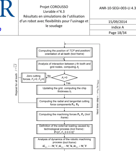
Described mechanism of chip formation and the machining force model (24) allow computing the dynamic behaviour of the robotic machining process where models of robot inertia and stiffness are discussed in the section 3 of the paper. The detailed algorithm that is used in numerical analysis is presented in 0, where the analysis of the robot dynamics is performed in the tool frame with respect to the dynamic displacement of the tool δtdyn fixed on the robot end‐effector around its position on the trajectory.
Repe
at for all teeth
Next time step τ : τ= τ0 : τ: τMA X Z j ,1 = 1 1 1
dyn c c dyn c c dyn c
− − −
= − − +
δt&& M C δt& M K δt M F
Figure 7 : Algorithm for numerical simulation of robotic machining process dynamics
2.5 Modèle du procédé FSW
Le principe du FSW consiste à apporter une énergie d’origine mécanique par l’action d’un outil à l’interface entre les pièces à souder. La liaison se crée de proche en proche à l’état solide. Le procédé FSW a été mis en œuvre, en premier lieu, dans les industries du transport, qui ont recours à l’aluminium pour alléger les structures mécaniques. En simulation, on utilise des modèles présentés dans le rapport Livrable 2.3 : Modèle exploitable pour la définition de la commande du robot. Les forces du soudage dépendent des paramètres physiques : matériaux des pièces à souder, épaisseur, forme et taille de l’outil, etc. Elles dépendent également de paramètres dynamiques : position et angle relatifs entre l’outil et la pièce, la vitesse avance, la vitesse de la rotation, etc. Les paramètres opératoires avec lesquels on contrôle la phase de soudage sont : • La vitesse d’avance de l’outil ou vitesse d’avance . • L’effort axial
appliqué sur l’outil suivant son axe de rotation. • La fréquence de rotation . • L’angle d’inclinaison de l’outil dénommé angle de tilt.
Projet COROUSSO Livrable n°4.3 Résultats en simulations de l’utilisation d’un robot avec flexibilités pour l’usinage et le soudage ANR‐10‐SEGI‐003‐LI 4.3 15/09/2014 indice A Page 19/34 Auteurs : A.K, A.P, S.G, S.C, F.L, G.A, J.Q
C
orousso
Figure 8 : Algorithm for numerical simulation of robotic machining process dynamics Les paramètres opératoires lors de la phase de soudage changent en fonction de l’épaisseur à souder, le matériau et la géométrie de l’outil. L’ensemble conditionne l’apport d’énergie, le flux de matière, la
formation du cordon, les propriétés mécaniques de l’assemblage et les efforts générés [Mishra 2005].
Modèle :
Selon les conditions dans notre étude, les forces extérieures pendant le procédé FSW peuvent être modélisées dans le simulateur comme suit :F
A . V
.
. F
F
A . V
. N . F
Par identification, on peut calculer les valeurs des coefficients du modèle avec la méthode des moindres carrés. On choisit les valeurs suivantes pour les simulations : 0,54; α 0,938 ; β 0,647; μ
0,021 et 13 . 10 ; α 0,596 ; β 0,37; μ 0,02 Évolution des variables principales en FSW • Identification des phénomènes limites aux frontières du domaine de fonctionnement • Évolution des composantes du torseur des interactions mécaniques outil/matière dans le domaine de fonctionnement • Modélisation statistique des composantes du torseur des efforts en fonction des principaux paramètres de conduite du procédé
3 RÉSULTATS DE SIMULATION EN USINAGE
3.1 Exemples avec un modèle d’usinage « Grid based Model »
CASE A: RIGID TOOL FIXATION. The objective of this case study is to understand the mechanics of the
tool/workpiece interaction, while any dynamic aspect related to the robot compliance is excluded from the analysis. In that case the applied feed rate and spindle rotational speed totally determine the position {xi, yi}, 1, z i= N of all tool cutting edges referred to robotic base frame at each instant of machining τ
(
)(
)
sin , cos 2 1 , 1, i f i i i z i z x v R y R N i i N τ φ φ φ τ π = + = = Ω + − = (28)The orientation αi of the i‐th tooth velocity vi can be defined by the feed rate vf and the spindle rotational
speed Ω at each instant as αi=atan2
(
(
v + vf Ωx)
vΩy)
with vΩx = ΩRsin ,ϕi vΩy = ΩRcosϕi. The angle αiprovides computing the chip thickness hi as the displacement of TCP corresponding to the one tooth period
2π ΩNz and referenced to the i‐th tooth, when it is situated inside the working material. If the given tooth is located outside the working material, the corresponding chip thickness hi is equal to zero. The following
expressions allow evaluating hi for all possible positions of the i‐th tooth on its path while machining 0, sin , 2 , 1, 2 sin , 2 i z i i i i f z f z i i f z x R h x R x v N i N v N x v N α π π α π ⎧ < ⎪ =⎨ ≤ < Ω = ⎪ Ω ≥ Ω ⎩ (29)
The advantage of the presented algorithm of computing the chip thickness is that different phases of tool/workpiece interaction illustrated in Figure 9 can be identified.
It should be mentioned that the phase of tool approaching to the workpiece corresponding to the zero machining force is not considered here. For the remaining phases a detailed analysis is presented below: The phase of tool engaging into the working material (phase I) corresponds to the variable contact area between the tool and the workpiece. The TCP during this phase is located always outside the workpiece. In fact, the phase I can be divided into two sub phases:
Projet COROUSSO Livrable n°4.3 Résultats en simulations de l’utilisation d’un robot avec flexibilités pour l’usinage et le soudage ANR‐10‐SEGI‐003‐LI 4.3 15/09/2014 indice A Page 21/34 Auteurs : A.K, A.P, S.G, S.C, F.L, G.A, J.Q
C
orousso
0 π/2 π 3π/2 2π −100 −50 0 50 100 150 [rotation period] -F x , [N ] vf Phase Ia 20π 20π+π/2 20π+π 20π+3π/2 20π+2π −100 −50 0 50 100 150 [rotation period] -F x , [ N ] 52π 52π+π/2 52π+π 52π+3π/2 52π+2π −100 −50 0 50 100 150 [rotation period] -F x , [ N ] 0 π/2 π 3π/2 2π −100 −50 0 50 100 150 [rotation period] Fy , [N ] 20π 20π+π/2 20π+π 20π+3π/2 20π+2π −100 −50 0 50 100 150 [rotation period] Fy , [N ] 52π 52π+π/2 52π+π 52π+3π/2 52π+2π −100 −50 0 50 100 150 [rotation period] Fy , [N ] (a) (b) (c) Figure 9 : Different phases of tool/workpiece interaction (case Nz=4) and corresponding machining forces; (a) – tool entry into the workpiece, only one tooth can be in contact with workpiece at the same time, (b) – increasing tool engagement into the workpiece, several teeth could be in contact with workpiece at the same time, (c) – slot machining with fully engaged tool. Phase Ia: In the beginning of milling operation a small area of workpiece is affected by the machining process. This fact and presence of two types of motion (feed, spindle rotation) form the case, when only one tooth can participate in cutting at the same time (Figure 9‐a). Such behaviour produces intermittent machining forces Fx
and Fy with the frequency ΩNz 2π Hz. The sub phase 1 is very limited in time and its duration depends on the feed rate, the spindle rotational speed and the number of teeth Nz. For example, if vf=4m/min, Ω=104rpm, Nz=4 the duration of phase Ia is only 0.04sec.
Phase Ib: It corresponds to a case, when several teeth can participate in cutting at the same time, but the TCP does not reach the workpiece border (Figure 9‐b). As a result an oscillatory periodic behaviour in machining forces Fx and Fy is observed. But, because of different number of currently working teeth, the force patterns
are not homogenous.
The phase of machining with fully engaged tool (Phase II) starts when TCP reaches the workpiece border (Figure 9‐c). In that case always the same number of teeth (nc=2 for the tool with Nz=4) is working at every
instant of cutting process. It produces harmonic periodic machining forces Fx and Fy with the frequency
2
Z π
behaviour of machining forces can be detected for whole process (Figure 10). The high frequency of such oscillation (for example, Ω=104rpm, Nz=4 give frequency of 667Hz) does not affect the motion of robot but it can be crucial for robot control system and should be considered in design of robotic machining process. 0 2 4 6 8 x 10⁻³ -100 -50 0 50 0.09 0.092 0.094 0.096 0.098 -100 -50 0 50 0.2 0.202 0.204 0.206 -100 -50 0 50 0 0.05 0.1 0.15 0.2 0.25 -100 -50 0 50 Time, [sec] F x ( W o rkp ie ce ->T o o l) , [N ] 0 2 4 6 8 x 10⁻³ 0 20 40 60 80 100 120 140 0.092 0.094 0.096 0.098 0 50 100 150 0.202 0.204 0.206 0.208 0 50 100 150 0 0.05 0.1 0.15 0.2 0.25 0 50 100 150 Time, [sec] Fy ( W o rkp ie ce ->T o o l) , [ N ] Figure 10 : Machining force patterns with average forces referenced to the frame {x, y}. CASE B: TOOL FIXATION WITH COMPLIANCE IN X DIRECTION. In contrast to Case A, the dynamic aspect of tool
motion associated with the robot compliance is considered here. Thus, at each instant of machining, the position xTCP is defined as a superposition of tool displacement xf due to feed and a dynamic displacement δx
due to compliance of the fixation: xTCP=xf +δx. The first component xf =vfτ is known at each instant of process while the second one depends on the current position of the tool regarding to the machining profile. In this case, the dynamic displacement δx can be obtained by reducing the equation (1) to a one‐dimensional problem and by introducing the damping related to the machining process and robot control algorithms
M x C x K x Fδ&&+ xδ&+ xδ = x (30)
where M is the equivalent mass of the tool fixation, Kx and Cx are its stiffness and damping respectively. The
damping Cx =2ζ K Mx is related to the damping factor ζ, which can be estimated experimentally. The machining force Fx acting in x direction, depends on the chip thickness h which in its turn depends on the
relative position between teeth of the tool and the workpiece (i.e. δx) at each instant of machining. Next, the position of the i‐th tooth in the robot base frame {x,y} can be easily determined:
xi=xTCP+Rsin ,ϕi yi =Rcos ,ϕi i=1,Nz.
Comparative analysis of this position with respect to the current machining profile defines the chip thickness hi
removing by i‐th tooth. But, the main issue here is to define whether i‐th tooth participates in cutting for given instant of process. For this reason, it is proposed to create a mesh on the workpiece, where each node j (
Projet COROUSSO Livrable n°4.3 Résultats en simulations de l’utilisation d’un robot avec flexibilités pour l’usinage et le soudage ANR‐10‐SEGI‐003‐LI 4.3 15/09/2014 indice A Page 23/34 Auteurs : A.K, A.P, S.G, S.C, F.L, G.A, J.Q
C
orousso
1, w j= N , Nw is the number of nodes) can be filled with “1” or “0”: “1” corresponds to nodes situated in the workpiece area with material, “0” corresponds to nodes situated in workpiece area that was cut away.
In order to define the number of currently cut nodes by the i‐th tooth, the previous instant of machining process should be considered. Let us define Ai as an amount of working material that is currently cut away by
the i‐th tooth (Figure 11). So, if node j filled with “1” is located inside the sector, it changes to “0” and Ai is
increasing by Δ Δ (Δss sx y x, Δsy are node steps in x and y directions respectively). Analysing all potential nodes
and computing Ai, the chip thickness hi, removed at given instant of process by the i‐th tooth, can be estimated
by hi= A Ri Δαi, i=1,Nz. The angle Δαi determines the current angular position of the i‐th tooth regarding
to its position at the instant τ‐Δτ (Δτ is the time step) and referred to the position of TCP at τ‐Δτ.
Figure 11 : Evaluating the tool/workpiece intersection Ai and computing the corresponding chip thickness hi
Here, in contrast to the previous case, the dynamic aspect of the tool motion allows:
Estimating of deviation in tool motion from the desired one because of the robot compliance in the feed
direction. It should be mentioned that this deviation affects the Cartesian stiffness of robot but does not influence the machining profile quality. For example, following parameters M=100 kg, Kx=3 10× 5 N/m, ζ=0.05, Nz=4, Ω=104 rpm, vf=4 m/min provide deviation in the feed direction of 0.13mm (Figure 12). But it is not
essential for this application.
Detecting of vibratory behaviour of tool motion while it is engaging into the workpiece. In some cases the low
frequency of such motion can excite robot natural frequency, destabilize machining operation and may even damage the tool or/and workpiece. For example, the milling process with following parameters M=100 kg, Kx=
5
3 10× N/m, ζ=0.05, Nz =4, Ω=104 rpm, vf=4 m/min generates vibration of f1=8.8Hz from the beginning of
0 0.2 0.4 0.6 0.8 1 1.2 -100 -80 -60 -40 -20 0 20 40 Time, [sec] F x ( W o rkp ie ce -> T o o l) , 0 0.2 0.4 0.6 0.8 1 1.2 0 20 40 60 80 100 120 140 Time, [sec] F y ( W o rkp ie ce -> T o o l) , 0 0.2 0.4 0.6 0.8 1 1.2 -0.2 -0.15 -0.1 -0.05 0 Time, [sec] D y nam ic di spl a cem ent δ x , [m m ] Figure 12 : Machining force patterns and TCP dynamic displacement in case of 1DOF model (M=100 kg, Kx= 5 3 ×10 N/m, ζ=0.05, Nz=4, Ω=104 rpm, vf=4 m/min).
More details on influence of the tool fixation parameters (M, Kx) on the dynamics of its motion during
machining are presented in Table 1, which covers the range of values for M, Kx computed for different
configurations of the robot KUKA KR 270. M, kg Kx, N/m τs, sec |xs|, mm PO, % f1, Hz 100 0.05 10× 6 1.2 0.80 52 3.5 100 0.30 10× 6 0.6 0.13 30 8.8 100 0.60 10× 6 0.5 0.07 23 12.4 100 1.00 10× 6 0.4 0.04 17 15.6 100 2.00 10× 6 0.4 0.02 11 22.6 150 2.00 10× 6 0.5 0.02 14 18.3 200 2.00 10× 6 0.5 0.02 18 15.6 Table 1: Influence of tool fixation parameters on the tool motion; τs is the settling time, PO is the overshoot, f1 is the first frequency of the tool dynamic displacement in feed direction ζ=0.05, Nz =4.104 rpm, vf=4 m/min As it can be observed from the table, changing the fixation parameters (i.e. the robot configuration) influences low frequencies (about 10 – 20 Hz) of the tool motion.
Projet COROUSSO Livrable n°4.3 Résultats en simulations de l’utilisation d’un robot avec flexibilités pour l’usinage et le soudage ANR‐10‐SEGI‐003‐LI 4.3 15/09/2014 indice A Page 25/34 Auteurs : A.K, A.P, S.G, S.C, F.L, G.A, J.Q
C
orousso
Suitable robot configurations to perform given machining operation could be defined. But, it should be mentioned that this one dimensional equivalent model presented here allows analysis of machining process dynamics in the feed direction only. In order to evaluate behaviour of the tool motion more closely to the real machining operation, this model should be extended. M r,xx=M r,yy, kg K r,xx=K r,yy, N/m |xs|, mm |ys|, mm f1x, Hz f1y, Hz 100 0.05 10× 6 0.80 2.61 3.2 2.2 100 0.30 10× 6 0.13 0.43 8.2 7.3 100 0.60 10× 6 0.07 0.22 12.4 11.4 100 1.00 10× 6 0.04 0.13 15.6 14.6 100 2.00 10× 6 0.02 0.06 22.4 21.5 150 2.00 10× 6 0.02 0.06 18.3 17.4 200 2.00 10× 6 0.02 0.06 15.6 15.6 Table 2: Influence of the tool fixation parameters on tool dynamic behavior; f1x, f1y are first frequencies of the tool dynamic displacement in x and y directions respectively; Nz =4. 104 rpm, vf=4 m/min CASE C: TOOL FIXATION WITH COMPLIANCE IN X AND Y DIRECTIONS. In this case, a dynamic aspect of tool motion in feed direction (x) and orthogonal to it (y) is considered. Then, similarly to the Case B, at each instant of machining process, the position of TCP is determined by xTCP=xf +δx y, TCP= yf +δy, where
, , ,
f f x f f y
x =v τ y =v τ . The dynamic displacements δx, δy could be obtained from the equation (1) which, in this case, is reduced to x y F x x x F y y y δ δ δ δ δ δ ⎡ ⎤ ⎡ ⎤+ ⎡ ⎤+ ⎡ ⎤ = ⎢ ⎥ ⎢ ⎥ ⎢ ⎥ ⎢ ⎥ ⎣ ⎦ ⎣ ⎦ ⎣ ⎦ ⎣ ⎦ r r Μ && C & Κ && & (31)
where Mr (2×2) is the equivalent mass matrix of the tool fixation, the matrices Kr (2×2) and C (2×2), where
, 2 , , ,
i j = ζi j i j i j
C K M characterize the fixation stiffness and damping respectively (which can be estimated
experimentally), Fx and Fy are the machining forces in x and y directions.
In contrast to the previous case, the position of the i‐th tooth at each process instant t includes dynamic components in both directions: xi =xTCP+Rsin ,ϕi yi= yTCP+Rcos ,ϕi i=1,Nz. The algorithm of computing the chip thickness hi for given position of tooth {xi, yi} is similar to Case B.
(that are not visible in Cases A, B) the robotic milling process is simulated for KUKA KR 270 robot with the following parameters 5 5 100 0 , kg, 3 10 0 , , 550 0 , 0 100 0 3 10 0 550 sec N kg m ⎡ × ⎤ ⎡ ⎤ ⎡ ⎤ =⎢ ⎥ =⎢ ⎥ =⎢ ⎥ × ⎣ ⎦ ⎣ ⎦ ⎣ ⎦ r r M K C . Here, the equivalent mass matrix Mr is computed in accordance with the method presented in the Section 2 of
this paper. The stiffness Kr is the structural stiffness of the robot, referred to its end‐effector. It should be
noted that in practice the non‐diagonal elements in these matrices are non‐zero. But, with this simplified case it is possible to identify qualitatively the dynamic nature of the tool behaviour in the direction (y) orthogonal to the feed. Simulation results corresponding to this case study are presented in Fig. 9.
It should be also stressed that the tool dynamic behaviour in the feed direction (x) is similar to the results, which were obtained in the Case B. The displacement in y‐direction has an essential dynamic component during the phase of tool engagement (Phase I) into the workpiece and becomes constant while machining with fully engaged tool. The corresponding frequency f1y=7.3Hz is comparable with the frequency f1x=8.2Hz of the
tool dynamic displacement in feed direction. More details on the tool motion during milling process regarding to the parameters of the tool fixation are presented in Table 2 (it covers the range of values for Mr,xx, Mr,yy, Kr,xx, Kr,yy computed for different configurations of the robot KUKA KR 270 using the methodology presented in
Section 2)
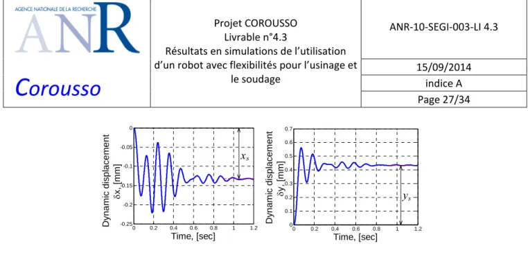
It should be noted that changing the robot configuration affects the tool dynamics in y direction which is crucial regarding to the quality of the final product. Hence, considering the tool displacement orthogonal to the feed direction is essential and the Case C gives more realistic results comparing Cases A and B. As it is shown in 0, the deviation (0.31 – 0.56mm) in machining profile from the desired one has a vibratory behaviour during the phase of tool engagement into the workpiece. Thus it cannot be suppressed by straightforward compensation methods and other compensation techniques should be proposed. 0 0.2 0.4 0.6 0.8 1 1.2 -100 -80 -60 -40 -20 0 20 40 60 Time, [sec] F x (W o rk p ie c e -> T o o l), [N ] 0 0.2 0.4 0.6 0.8 1 1.2 0 20 40 60 80 100 120 140 160 Time, [sec] F y ( W or k p ie c e -> T ool ), [N ]
Projet COROUSSO Livrable n°4.3 Résultats en simulations de l’utilisation d’un robot avec flexibilités pour l’usinage et le soudage ANR‐10‐SEGI‐003‐LI 4.3 15/09/2014 indice A Page 27/34 Auteurs : A.K, A.P, S.G, S.C, F.L, G.A, J.Q
C
orousso
0 0.2 0.4 0.6 0.8 1 1.2 -0.25 -0.2 -0.15 -0.1 -0.05 0 Time, [sec] Dyna m ic di spl a ce me n t δx, [mm ] 0 0.2 0.4 0.6 0.8 1 1.2 0 0.1 0.2 0.3 0.4 0.5 0.6 0.7 Time, [sec] Dy nam ic dis p la cem e nt δy , [ mm] Figure 13 : Machining force patterns and TCP dynamic displacements in case of 2DOF model (Mr,xx=Mr,yy=100 kg, Kr,xx=Kr,yy=3 ×10⁵ N/m, Nz=4, Ω=104 rpm, vf=4 m/min).
3.2 Exemple avec un modèle d’usinage à effort spécifique de coupe
Le modèle d’effort de coupe choisi est adapté à une opération de détourage. L’outil est une fraise cylindrique revêtue de grains abrasifs. L’outil est solidaire de la partie terminale de l’outil et son axe de rotation est perpendiculaire au plan du travail. On suppose que la trajectoire du bout d’outil reste dans le plan , . Les forces sont exercées au point par la pièce sur l’outil qui est fixé au 6ème corps du robot. Les forces peuvent être calculées par une modélisation des efforts de coupe. En première approximation, on peut considérer que la force de coupe est proportionnelle à la section de matière enlevée et à l’effort spécifique de coupe . Lorsque le robot est soumis à un effort, les raideurs en torsion non infinies entraînent un déplacement de celui‐ci et donc une modification de la section de matière enlevée comme le montre la Figure 14. On obtient l’effort de coupe par :
avec la profondeur de coupe et représentant la largeur de matière enlevée. L’effort spécifique
de coupe dépend de la matière, de l’outil et de la vitesse d’avance qui est imposée par le robot. Dans le cas du détourage considéré sur la Figure 14, la vitesse d’avance est définie par qui dépend à l’instant t des déformations du robot dans la direction . La modélisation de la coupe des matériaux composites n’a pas fait l’objet de travaux aussi approfondis que la coupe des métaux. Par analogie avec les modèles de coupe considérant un cisaillement primaire, l’effort spécifique peut être exprimé par :
avec un coefficient dépendant du matériau et qui sera déterminé expérimentalement et m l’indice viscoplastique dans les conditions données de température et de coupe.
L’e de pre Le effort norma s matériaux emière appro vecteur des l de coupe e x composites oximation, o forces extér Figure 14 est obtenu à s sont assez on peut adme rieures qui s’ : Modélisatio partir de l’é z éloignées d ettre que : ’appliquent d on de l’usinage étude des fro de celles de donc au robo e pour le déto ottements. Ic e l’usinage c ot est défini ourage. ci encore, les onventionne par s conditions el des méta
.
de l’usinage ux, mais en e n