Technology researchers and makes it freely available over the web where possible.
This is an author-deposited version published in: https://sam.ensam.eu Handle ID: .http://hdl.handle.net/10985/19539
This document is available under CC BY license
To cite this version :
Mattias SCHEFFLER, Nazih MECHBAL, Marc REBILLAT, Eric MONTEIRO, Nicolas BARABINO Sensorless Nonlinear Stroke Controller for an Implantable, Undulating Membrane Blood Pump -In: 58th Conference on Decision and Control, France, 2019-12 - Proceedings of the 58th Conference on Decision and Control - 2019
Any correspondence concerning this service should be sent to the repository Administrator : [email protected]
+
Abstract— This paper describes an original methodology to operate a new nonlinear vibrating membrane pump, actuated by a moving magnet actuator without the use of a motion sensor, in the scope of cardiac assistance. A nonlinear mathematical model of the system is established and used to parametrize a nonlinear position observer that uses the coils current as an input and which output is a feedback to a stroke controller. Actuator’s parameters are identified by a recursive least square algorithm and direct measurements. Finally, a numerical experiment illustrates the implementation of the algorithm and its possible applications.
Index terms— Biomedical, Control Application, Left Ventricular Assist Device, Non-linear system, observer, sensorless control.
I. INTRODUCTION
Chronic heart failure (CHF) is a medical condition where the heart is unable to pump blood sufficiently to meet body needs. It is a common, yet costly and often fatal condition. It is estimated that overall 2% of adults in the western hemisphere suffer from heart failure [1]. Depending on the severity of CHF, therapies vary from dietary restriction to heart transplantation. For the most advanced CHF patients, in cases where prompt heart transplantation is impossible due to patient ineligibility or donor organ scarcity, a left ventricular assist device (LVAD) can be surgically implanted. It consists of a pump whose inlet is connected to the ventricle while the outlet is connected to the aorta. Blood is directly pumped from the ventricle and ejected to the aorta, thus restoring blood perfusion. It differs from total artificial hearts such as [2] in that no part of the heart is removed during surgery.
Several pumping technologies have been adapted to heart assistance prior to this submission, and all are subject to common critical requirements: (i) pump flow must be sufficient to restore perfusion; (ii) the system must not be subject to failure when used for several months or even years; (iii) the pump must be small-sized so it can be surgically implanted inside the thorax and last, (iv) the system efficiency must be high enough for it to be powered by portable batteries for several hours, to guarantee patient autonomy.
The first generation of LVADs was blood-filled sacs emptied by an air compressor or an electrically driven pusher
plate like [3]. Although able to produce a high-fidelity blood flow which was close to natural heart flow rate, pulsatility and low blood damage, those are not used anymore due to their lack of reliability. The second and third generations consist of rotative pumps such as in [4]. More reliable and with a reduced size, these pumps have improved patient survival rates. However, this improvement is at the expense of a drastic loss of flow pulsatility control as these pumps are operated at an almost constant rotation speed. New medical complications appeared, largely caused by the continuous operation of these pumps [5]. Ventricular suction, described in [6], may occur and must be avoided via control strategies such as [7]. Mechanical haemolysis due to blood cell shear stress near the pump’s rotating blades is now a design issue. Thrombus formation inside the pump and gastrointestinal bleeding require medical attention [8]–[10]. All these pumps require control laws to ensure safe operation, which is a challenge because adding sensors in the human body or to the pump itself is always detrimental to biocompatibility.
This contribution deals with the control of a new type of LVAD, based on an undulating membrane pump technology. It aims to produce near instantaneous flow modulations while at the same time keeping the required power surge at a reasonable level, and an implantable size. Both its design and operation principle differ from existing LVADs as it does not contain any rotating parts that have a momentum of inertia that significantly limits the rate at which flow can be changed. Indeed, the fluid is propelled by the undulation of a membrane made of a lightweight polymer material. The miniaturization of this technology into an LVAD requires to solve several issues. The present contribution focuses on control issues raised by this choice of technology.
II. THE IMPLANTABLE UNDULATING MEMBRANE PUMP
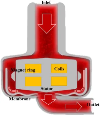
This technology, originally patented in [11] is made of an inlet, an outlet and a pump body that is the operation space bounded by rigid walls where a deformable membrane is excited at one end by a periodic force exerted normally to the membrane surface [12], [13]. The excitation results in a deformation wave that propagates from the excited end of the membrane, close to the inlet, to the opposite end, which is near the outlet. The propagation of the wave transmits energy to the fluid to create a flow and pressure gradient in the direction of the propagation [11].
In our application, the generated periodic excitation is made by an axisymmetric, moving magnet actuator (see
Figure 1 and Figure 2). This actuator consists of two coils
wound inside a stator that are powered by alternative current, and a permanent magnet moving ring to which the excited
Sensorless Nonlinear Stroke Controller for an Implantable,
Undulating Membrane Blood Pump
Mattias Scheffler, Nazih Mechbal, Marc Rebillat, Eric Monteiro, Nicolas Barabino, Member, IEEE
M. Scheffler, N. Mechbal, M. Rebillat and E. Monteiro are with the PIMM laboratory, UMR CNRS Le CNAM, HESAM universite, 151, boulevard de l’Hopital, 75013 Paris, France (e-mail: [email protected], [email protected], [email protected], [email protected])
N. Barabino is senior R&D manager at CorWave SA, 17, rue de Neuilly, 92110, Clichy, France (e-mail: [email protected])
Figure 1. Commercial schematics of the pump. Flow direction is indicated by red arrows
end of the membrane is attached. The magnet ring is centred around the stator and kept around a rest position by a set of springs. The design of a prototype that fulfils all the requirements mentioned above necessitates to overcome many challenges in terms of mechanical design and manufacturing process. It is also a challenge from a control perspective because unlike rotary pumps, the operation point of a vibrating membrane pump is set by the frequency and amplitude of membrane excitation. Indeed, the higher the frequency or the stroke is, the higher the pressure head will be. As a consequence, the stroke needs to be set accurately with sufficient speed to be able to switch the operating point of the pump fast enough to recreate a pulse synchronized to heartbeats. At the same time, it must be restrained so as not to damage either the membrane, the springs or the blood by excessive stress. Overstress of the mechanical parts can be caused by overpowering the actuator or by the effect of perturbation forces induced by the remaining activity of the left ventricle. Due to the specific medium (blood) in which the pump is operating, it is highly recommended to avoid adding position, velocity or acceleration sensors that would significantly increase the complexity and size of the pump.
Approaches that bypass the use of motion sensors have been studied for similar actuators or applications. One of those consists in measuring current ripple generated by a PWM voltage input [14] to estimate an equivalent circuit inductance that is related to the magnet position. This method only works if the magnetic parts’ velocity is close to zero which is not the case in the vibrating membrane pump that operates at frequencies close to 100 𝐻𝑧. Other methods compute the back electromotive force (𝑏𝑎𝑐𝑘 𝑒𝑚𝑓, proportional to velocity) from an inverted equivalent electric
circuit [15] and directly integrate the estimated speed to get the position. This last method only requires knowledge of electrical parameters and no information about the mechanical subsystem of the actuator are needed. However, coil current derivative must be computed which is not trivial in a noisy environment. Latham et al.[16] present a velocity observer to estimate the 𝑏𝑎𝑐𝑘 𝑒𝑚𝑓 that does not rely on computing any time derivative. The resulting position from integrating the estimated velocity [15]–[17] is sensitive to measurement bias that propagates into the velocity estimation which results in drift when integrated. This effect can be bounded by adding another stage to the observer as proposed in [18]. This stage adds partial knowledge about the mechanical subsystem of the actuator, and is robust to unknown, bounded forces. However, these studies are limited to a linear domain of the actuator, where the parameters of the equivalent electric circuit of the actuator can be approximated as constants. This approximation is valid for these applications, but not in our case because the actuator size is made as small as possible and it is expected to perform along its whole stroke range.
This contribution thus aims to synthesize a stroke nonlinear controller for the pump that will only rely on actuator current measurement. It will be robust to pressure and flow changes inside the pump head and allow fast change of pump operation point. To do so, a two-stage, nonlinear position observer is developed based on a reduced order nonlinear model of the electromagnetic actuator. As the actuator is very small regarding its performance requirements, we cannot make the linear approximation of the equivalent electric circuit that is commonly made. To meet nevertheless the required operation range of the controller, parameters’ variations regarding state variables will be included in the model and the observer. Means to identify actuator’s nonlinear model are given by a recursive least squares (RLS) so they can be incorporated in a into the observer. A forgetting factor is included in the RLS to capture model parameters’ variations regarding state variables. We propose to validate our approach with numerical simulations of the identification process and then of the controller.
The paper is organised as follows: Section III introduces the different elements of the pump model. Section IV and V synthetize the position observer and pump’s stroke controller. Section VI details the identification scheme that is used and finally Section VII shows the results of the implementation and a comparison of the expected operation range of the pump when the non-linearities of the actuator are included or not.
III. MODELLING OF THE SYSTEM
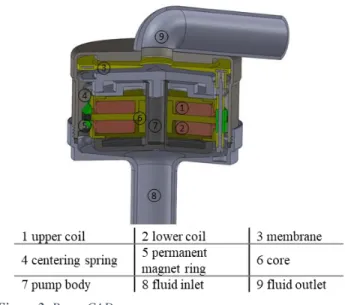
The pump is a complex system that is represented in Figure
2. To help designing the stroke controller we set up a model
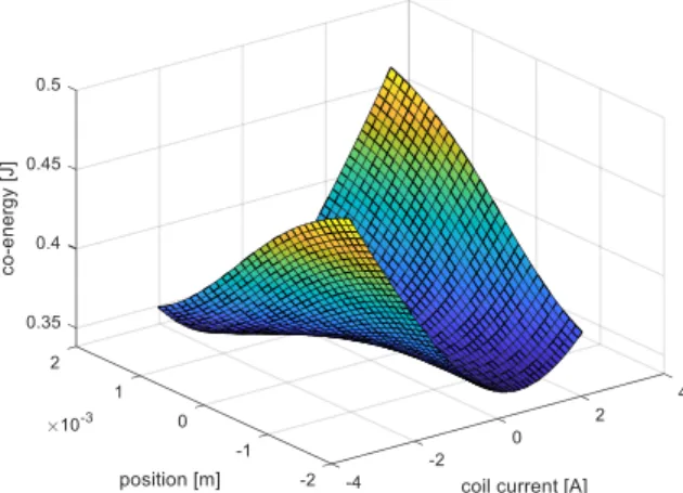
of the pump. D. Wiedemann in [19] proposes a clear methodology to transform a finite elements method model (FEM) of a moving magnet actuator into a lumped parameters model represented by a system of ODEs. We do propose to follow the same approach to transform the complex system shown in Figure 2 into the simpler lumped parameters model of Figure 4. It relies on the computation of the co-energy 𝑊 of the system for various position of the magnet and coils
Figure 2. Pump CAD
current as depicted in Figure 6. The FEM model is set up by following the methodology presented in [20] on a commercial software (MagNet 2D/3D). An overview of the simulated geometry and mesh is visible in Figure 3. In our case we simulate the static response of the actuator to a prescribed current density inside the coils area, and magnet ring position. Before running the simulation, a mesh convergence study has been done. In areas with the most flux’s variations (i.e. in the airgap between the magnet and the core), the size of the elements is reduced.
Figure 3. Simulated geometry and mesh overview
With that resulting co-energy variable (seen in Figure 6) a lumped parameters model is deduced from the FEM model. The partial derivatives of 𝑊 are computed and identified to the parameters of an equivalent circuit which is expressed as (1). The one degree of freedom motion equation of the magnet ring of the pump is given in (2):
𝑉𝑖𝑛(𝑡) = 𝑅𝐼 + 𝐿(𝑥, 𝐼) 𝑑𝐼 𝑑𝑡+ 𝐸(𝑥, 𝐼) 𝑑𝑥 𝑑𝑡 (1) 𝑚𝑥̈(𝑡) = 𝐹𝑚𝑎𝑔(𝑥, 𝐼) + 𝐹𝑠(𝑥) + 𝐹𝑚𝑒𝑚𝑏(𝑡) (2) 𝐹𝑠(𝑥) = 𝑎𝑥3+ 𝑏𝑥 (3)
where 𝑉𝑖𝑛, 𝑥, 𝐼, 𝑅, 𝐿 and 𝐸 are respectively the input voltage,
magnet position, coils current, coils resistance, coils inductance and 𝐸 the 𝑏𝑎𝑐𝑘 𝑒𝑚𝑓 factor. Springs reaction force 𝐹𝑠 (Figure 5) is identified to a third-degree polynomial of 𝑥
given in (3). It takes into account design induced nonlinearities that are measured on a pull tester
𝐿, 𝐸, 𝐹𝑚𝑎𝑔 are related to 𝑊 by the following relationships that
are demonstrated in details in [19]:
𝐿(𝑥, 𝐼) =𝜕 2𝑊(𝑥, 𝐼) 𝜕𝐼2 (4) 𝐸(𝑥, 𝐼) =𝜕 2𝑊 𝜕𝑥𝜕𝐼 (5) 𝐹𝑚𝑎𝑔(𝑥, 𝐼) = 𝜕𝑊(𝑥, 𝐼) 𝜕𝑥 (6)
Those relations between co-energy and the parameters of the lumped model are interesting for two reasons. First, it is a good test to validate the FEM simulation, because the parameters computed from partial derivatives of 𝑊 should have limited variations from point to point. Then the knowledge of the variation of those parameters will reveal the limits of the linear operation range of the actuator.
Figure 4. Schematic representation of Eqs (1) and (2)
We assume that the membrane force 𝐹𝑚𝑒𝑚𝑏 is bounded and
piecewise continuous. Its effects will be dealt with by a robust observer. Indeed, the fluid-structure interaction between the membrane and the fluid is too complex to be reduced to an analytic function. This is a source of problems because it forces us to find a control approach that is robust to the variations of this almost unknown force. Then to test numerically the developed controller we will have to choose an ersatz force to enabling the realization of simple tests. This means that we should expect differences between the numerical test bench, and an implementation on a real prototype.
Figure 5. Springs reaction force polynomial identified from measurements
IV. POSITION OBSERVER FOR SENSOR-LESS CONTROL
Now that a model of the system is provided, we need to design a stroke controller. The variable to be controlled is magnet position 𝑥, however, as we mentioned above it is not possible to measure 𝑥 with a sensor. Hence, we propose to build a position observer that will allow to control the excitation of the membrane with an estimate of 𝑥. The previous section shows that our system presents unmodelled forces. This means that our observer has to be robust to
Figure 6. Co-energy computed from the FEM model, displayed as a function of magnet ring’s position and coil current. unmodelled dynamics. As it is possible to directly measure current (with a probe placed inside the power electronics, i.e. outside patient’s body), and the electric dynamics is well known, we will rely mostly on Eq (1), ([16], [18]). This equation can be used to create an estimate of velocity, that can be integrated to the position [15]. However, any bias in current measurement will result in a constant error of velocity, that will result in a drift of position. This situation can be improved if we can bound position error with Eq (2). We also need to find an acceptable way to compute current derivative that will not amplify measurement noises. In order to cope with these constraints, we propose a two stage strategy (Figure 7):
The first stage is a velocity estimator (𝑥̇̂) that is directly deduced from Eq. (1). It includes a current derivative estimator to tackle the current derivation problem.
The 2nd stage is a position observer (𝑥̃) that takes
current measurement and the velocity estimate of the 1st stage as inputs.
From (1) the velocity estimator can be expressed as: 𝑥̇̂ = 1
𝐸(𝑥̃, 𝐼)(𝑉𝑖𝑛− 𝑅𝐼 − 𝐿(𝑥̃, 𝐼) 𝑑𝐼
𝑑𝑡) (7)
It is obvious that the current derivative in (7) will make the estimation extremely sensitive to measurement noise if left as it is. Different solutions exist to deal with this estimation problem such as low pass filtering or more elaborated techniques ([17]). Following the work of [21]–[23] we propose a derivative estimator:
𝑑𝐼 𝑑𝑡 ̂ (𝑡) = − 6 𝑇3∫ (𝑇 − 2𝜏)𝐼(𝑡 − 𝜏)𝑑𝜏 𝑡 𝑡−𝑇 (8) with 𝑇 the length of the integration windows. This estimation is straightforward to implement as a discrete FIR filter by using the trapezoidal method:
𝑑𝐼 𝑑𝑡 ̂ (𝑘𝑇𝑠) = − 6 (𝑁𝑇𝑠)3 ∑𝑁𝑖 = 0𝑤𝑖(𝑁𝑇𝑠− 2𝑖𝑇𝑠)𝐼(𝑘𝑇𝑠− 𝑖𝑇𝑠)𝑑𝜏 (9)
𝑁 being an integer chosen so that 𝑇 = 𝑁𝑇𝑠, 𝑤0 = 𝑤𝑁= 𝑇𝑠
2
and 𝑤𝑖= 𝑇𝑠 ( 𝑖 = 1, … 𝑁 − 1).
Based on the idea proposed in [18], the 2nd stage of the
observer is designed. If 𝑥̃ and 𝑥̇̃ are the observed position and velocity, the observer is expressed as:
[𝑥̇̃ 𝑥̈̃] = 𝑨 [ 𝑥̃ 𝑥̇̃] + [ 0 𝐹(𝑥̃, 𝑥̇̃, 𝐼)] + [ 𝑘1 𝑘2 ] (𝑥̇̂ − 𝑥̇̃) (10) with 𝑨 a constant square matrix regrouping the linear terms of Eq. and 𝐹 the function regrouping the nonlinear elements, and 𝑘1 and 𝑘2 two gains to be chosen to guarantee:
lim
𝑡→∞[
𝑥 − 𝑥̃
𝑥̇ − 𝑥̇̃] = 𝟎 (11)
V. POSITION CONTROLLERS
Figure 7. Multistage control diagram
From the observed position a stroke controller that will satisfy the requirements (setting the excitation to a desired stroke 𝑆𝑑,
for a given frequency 𝑓𝑑 while limiting overshoots) is
designed. It consists of a feedforward and a PI controller. The feedforward is a linearization of Eqs (1) and (2) around the resting point (𝑥 = 0, 𝐼 = 0), given in (12) and (13). It takes as input the desired position 𝑥𝑑 at each time step to compute
𝑉𝑖𝑛 as: 𝑉𝑖𝑛= 𝑅𝐼𝑑+ 𝐿(0,0) 𝑑𝐼𝑑 𝑡 + 𝐸(0,0) 𝑑𝑥𝑑 𝑑𝑡 (12) 𝜕𝐹𝑚𝑎𝑔 𝜕𝐼 (0,0)𝐼𝑑 = 𝑚𝑥̈𝑑− 𝜕𝐹𝑠𝑝𝑟𝑖𝑛𝑔𝑠(0) 𝜕𝑥 𝑥𝑑− 𝛼 𝑑𝑥𝑑 𝑑𝑡 (13) where 𝛼 represents a viscous damping coefficient that could be related to the membrane force. We choose to keep a linear formulation of the feedforward as its effect will be predominant only at startup or a change of operation point. The reference signal 𝑥𝑑 is generated to be sufficiently smooth,
in such a way to not create any discontinuity in the feedforward during startup or change of desired stroke 𝑆𝑑 or
frequency 𝑓𝑑 (which is supposed to happen frequently in order
to change the operation point of the pump) To do so the transfer function 𝐻(𝑠) is introduced:
𝑥𝑑(𝑡) = 𝑆(𝑡)sin (𝜑(𝑡)) (14) 𝜑(𝑡) = 2𝜋𝑓(𝑡) (15) 𝑆(𝑠) 𝑆𝑑(𝑠) (𝑠) = 𝑓(𝑠) 𝑓𝑑(𝑠) = 𝑘𝑓 3 (𝑠 + 𝑘𝑓)3= 𝐻(𝑠) (16) where 𝑘𝑓 is a positive, real number that guarantee the stability
of 𝐻(𝑠).
Then, the remaining errors due to un-modeled dynamics are cancelled by a PI controller that adjust the amplitude of the excitation. One way to estimate this amplitude is to define an
amplitude estimator 𝑆̂(𝑡) that is valid if 𝑥(𝑡) is sufficiently close to a sinus function, i.e.:
𝑆̂(𝑡) = √𝑥̂(𝑡)2+ 𝑥̂ (𝑡 − 1
4𝑓(𝑡))
2
(17)
VI. PARAMETERS IDENTIFICATION
In order to validate the model of section III and adjust it with experimental data, an estimation of the electric parameters (𝑅, 𝐿(𝑥, 𝐼), 𝐸(𝑥, 𝐼)) is developed. A recursive least square estimation scheme that include a forgetting factor is used. As the weight of the oldest samples will gradually be reduced, we will see time variation of the electric sub-model. By adjusting the current and position of the magnet, we will run the estimation process for every point that was simulated with the FEM model and compare the resulting inductance and 𝑏𝑎𝑐𝑘 𝑒𝑚𝑓.
Parameters 𝑅, 𝐿 and 𝐸 are unknown and slowly time varying. The variables 𝑉𝑖𝑛, 𝐼 and 𝑥 are piecewise continuous
and bounded, and all equal to zero at 𝑡 = 0. The problem is set by integrating (1) over time, i.e.
𝐼 =1 𝐿∫ 𝑉𝑖𝑛+ 𝑅 𝐿∫ 𝐼 + 𝐸 𝐿𝑥 (18)
which can be expressed as: 𝑦 = 𝚿𝑻𝜽 (19) 𝚿𝑻= [∫ 𝑉 𝑖𝑛 ∫ 𝐼 𝑥] (20) 𝜽 = [1 𝐿 𝑅 𝐿 𝐸 𝐿] (21)
For each sample 𝑛 > 0,
𝜽̂𝒏= 𝜽̂𝒏−𝟏+ 𝑲𝒏(𝑦𝑛− 𝑦̂𝑛) (22)
𝑦̂𝑛= 𝚿𝐧𝑻𝜽̂𝒏−𝟏 (23)
where 𝑲𝒏 is updated at each time step to minimize the least
square error function.
VII. RESULTS
The co energy result of the FEM simulations (Figure 6) is computed for magnet positions and coils currents that are part of the operation range of the pump. The partial derivatives that make up the inductance, the back emf coefficient and the magnetic force are computed (Figure 8). Their computation shows that the FEM model is sufficiently performant to guarantee the required smoothness of the parameters after derivation.
A numerical model of the pump and the controller is built under Matlab/Simulink to test the implementation of the controller and motor parameters’ identification before allocating resources to build a dedicated test setup for the implementation on the real pump prototype (see Figure 9). Actuator’s model is compared to measurement and adjusted accordingly. Springs’ reaction force is measured by using a pull tester. The same pull tester in Figure 9 is also used to measure the magnetic force of the actuator by applying an arbitrary constant electric current on actuator’s coils while
Figure 8. Co-energy, magnetic force, back emf and inductance from FEM simulation and partial derivation
measuring force. Near the rest point of the actuator, the linear approximation of motor parameters gives
Fmag(0, I) = AI (24)
𝐸(0, 𝐼) =𝑑𝐹𝑚𝑎𝑔
𝑑𝐼 = 𝐴 (25)
with A a positive constant. Electric inductance and resistance can be estimated with a LRC meter when the magnet ring’s motion is blocked to cancel the effect of the back emf. As LRC meters’ input current is limited (< 20 𝑚𝐴), inductance can only be estimated in this limited area. In quantitative term, measurements near the rest point give 𝐿 = 33 mH, and 𝐴 = 18 𝑁𝐴−1
, while simulation gives 𝐿 = 24 mH and 𝐴 = 24 𝑁𝐴−1. As membrane force is currently poorly known we
propose to emulate it by a viscous friction term µ that is a sensible first approximation:
𝐹𝑚𝑒𝑚𝑏𝑟𝑎𝑛𝑒(𝑡) = 𝜇(𝑡)𝑥̇ (26)
Using the verified lumped parameters model deduced from FE simulation, we test the whole strategy for identification and stroke control. In particular, we aim to compare different observer implementations to show the interest of using varying electric parameters instead of linear approximations.
Figure 9 Left: actuator mounted on the pull tester. Right: Pump mounted on test bench. Motion measurement is made a laser sensor.
A. Identification results
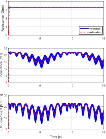
The result of the identification is shown in Figure 10. To guarantee a quick convergence two excitation signals are applied to the actuator. A voltage excitation that contains a high frequency (500 𝐻𝑧) square wave voltage that makes the inductance’s voltage to never be close to zero, and a low frequency (0.1 𝐻𝑧) sinus component for resistance’s voltage and to reach every position. To ensure that back emf is represented in the response, an external sinus force is simulated at 50 𝐻𝑧. To filter out high frequency variations as well as eventual noise, while capturing the low frequency variations of the parameters 𝜆 is set to 0.999 via a trial and error approach. The recursive least square identification was run with different initial conditions. Measurement errors (noises, bias, gain) were simulated to verify that their effects would not hinder convergence and help to diagnostic future experimental issues. RLS algorithm can filter out high frequency noises very easily, but gain errors lead to over or underestimation of parameters while bias and low frequency noise increase estimation error over time.
Figure 10. Identification of resistance, inductance and electromotive force. Blue lines: varying parameters from co-energy derivation. Red dashes: identification results.
B. Sensor-less control implementations and evaluation
A discrete version of the controller is implemented on Simulink to emulate what would be done by compiling it on a hardware target. As the frequency response of the derivative estimator of Eq (9) depends of the length of the integration
window and the sampling rate, and the signals to derivate may have frequency up to 100 Hz, we choose to set 𝑇𝑠= 2. 10−5𝑠
and 𝑁 = 6 (i.e. integration window of 1,2. 10−4𝑠), which is
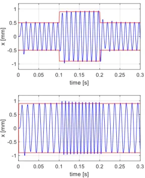
in this case a good trade between noise attenuation and performances. Figure 11 displays the response of the actuator from startup at 𝑡 = 0 𝑠 to a nominal constant operation point (a constant amplitude and frequency). Current and position are both reasonably sinusoidal, and after a transition period, the amplitude of position reaches the desired amplitude, and the observer output keeps track of the variation of position. In Figure 12 two cases of change of operation points are depicted (a change of frequency and a change of stroke). Those are two
Figure 11. System response to a desired stroke of 0.9 mm at 90 Hz. Top: coils’ current. Bottom: position of the mobile parts (red dashes: desired stroke, blue line: real position, green: observed position)
ways to increase or decrease pump flow. We can notice that overshoots appear during a change of stroke. If not kept below a safe level, they could create overstress that could damage the membrane and the springs. This can be avoided by making the desired stroke signal change smoother. In figure 13 a comparison between two observers is given. These observers are different through their first stage. One is the velocity observer developed in [16]. The other the one is designed from Eq (7). In each case, inductance and back emf are implemented as constant approximation and as functions. As the controller must maintain stroke over a wide range of strokes and frequencies, and different reaction forces of the membrane that are unknown we need to test combinations of
those three parameters to evaluate the performance of the controller. To do so we emulate the variation of the membrane force according to flow and pressure inside the pump head by varying µ, and we create an error variable 𝑒 that is evaluated over a range of strokes, frequency and µ:
𝑒(𝑆𝑑, 𝑓𝑑) = max
µ (|𝑆𝑑− 0.5(max 𝑥 − min 𝑥)|) (27)
where max 𝑥 𝑎𝑛𝑑 min 𝑥 are computed from one period of oscillation. This formulation of 𝑒 can be compared to a maximal admissible error 𝜀 : every operation point [𝑆𝑑, 𝑓𝑑]
which presents 𝑒 < 𝜀 can be reached safely (stroke will be maintained to deliver the required flow without the risk of damaging the device by an overshoot). With this performance indicator, we can see that taking into account the variations of the inductance and back emf in the velocity estimator (or observer in the case of [16]) results in an increase of the operation range of the stroke controller.
Figure 12. System’s reaction to a change of operation point. Top change of strokes. Bottom: change of frequency. Red lines: desired stroke, blue lines: real position.
CONCLUSION AND FUTURE WORK
In this work, we have demonstrated that it is possible to synthetize a stroke controller and assess its performance with a numerical experiment. This process requires to compute the co-energy of the actuator that allows to build a dynamic model of the actuator that is accurate and quick to run. From the resulting lumped parameters model it is possible to formulate a position observer that keeps the error bounded, that include magnetic induced non-linearities of the actuator. At last we propose a way to identify the variation of actuator’s parameters that could be done in an experiment. In the same perspective of being able to test on a live prototype we create numerical experiments that evaluate the performance of the controller according to requirements. It shows that it is beneficial to
include the non-linearities of the actuator into the observer as it widens the range of the operation of the system, whatever the choice of algorithms. Currently, experimental implementation is in progress, in order to validate the approach before testing it in vivo.
Figure 13. Stroke output error map of the system for different observer implementations. Green area: error below 0.1 mm. Red area: error above 0.1 mm. Top: 1st stage uses velocity
estimator. Bottom: 1st stage is made according to [16]. Left:
constant inductance and back emf. Right: variable inductance and back emf
ACKNOWLEDGMENT
We would like to thank all the engineers and technicians working at CorWave who supported us to present this contribution.
REFERENCES
[1] G. Savarese, L. H. Lund, Department of Cardiology, Karolinska University Hospital, Stockholm, Sweden, L. H. Lund, Division of Cardiology, Department of Medicine, Karolinska Insitutet, Stockholm, Sweden, and Department of Cardiology, Karolinska University Hospital, Stockholm, Sweden, “Global Public Health Burden of Heart Failure,” Cardiac Failure Review, vol. 3, no. 1, pp. 7–11, 2017.
[2] M. J. Slepian, Y. Alemu, J. S. Soares, R. G. Smith, S. Einav, and D. Bluestein, “The SyncardiaTM total artificial heart: in vivo, in vitro, and computational modeling studies,” Journal of Biomechanics, vol. 46, no. 2, pp. 266–275, Jan. 2013.
[3] N. Yuan et al., “The Spectrum of Complications Following Left Ventricular Assist Device Placement,” Journal of Cardiac Surgery, vol. 27, no. 5, pp. 630–638, Sep. 2012.
[4] O. Castellanos, K. Faulkner, and G. Ramina, “Generations of Left Ventricular Assist Devices: The HeartMate Family,” p. 6. [5] S. N. Purohit, W. K. Cornwell, J. D. Pal, J. Lindenfeld, and A. V.
Ambardekar, “Living Without a Pulse: The Vascular Implications of Continuous-Flow Left Ventricular Assist Devices,” Circulation: Heart Failure, vol. 11, no. 6, p. e004670, Jun. 2018.
[6] K. Reesink et al., “Suction Due to Left Ventricular Assist: Implications for Device Control and Management,” Artificial Organs, vol. 31, no. 7, pp. 542–549, Jul. 2007.
[7] Y. Wang, S. C. Koenig, M. S. Slaughter, and G. A. Giridharan, “Rotary Blood Pump Control Strategy for Preventing Left Ventricular Suction:,” ASAIO Journal, vol. 61, no. 1, pp. 21–30, 2015.
[8] S. S. Najjar et al., “An analysis of pump thrombus events in patients in the HeartWare ADVANCE bridge to transplant and continued
access protocol trial,” The Journal of Heart and Lung Transplantation, vol. 33, no. 1, pp. 23–34, Jan. 2014. [9] S. Crow et al., “Gastrointestinal bleeding rates in recipients of
nonpulsatile and pulsatile left ventricular assist devices,” The Journal of Thoracic and Cardiovascular Surgery, vol. 137, no. 1, pp. 208–215, Jan. 2009.
[10] D. Malehsa, A. L. Meyer, C. Bara, and M. Strüber, “Acquired von Willebrand syndrome after exchange of the HeartMate XVE to the HeartMate II ventricular assist device,” European Journal of Cardio-Thoracic Surgery, vol. 35, no. 6, pp. 1091–1093, Jun. 2009. [11] J. B. Drevet, “Vibrating membrane fluid circulator,” US
2001/0001278 A1, 17-May-2001.
[12] H. Feier et al., “A Novel, Valveless Ventricular Assist Device: The FishTail Pump. First Experimental In Vivo Studies,” Artificial Organs, vol. 26, no. 12, pp. 1026–1031, Dec. 2002.
[13] M. Perschall, J. B. Drevet, T. Schenkel, and H. Oertel, “The Progressive Wave Pump: Numerical Multiphysics Investigation of a Novel Pump Concept With Potential to Ventricular Assist Device Application: THE PROGRESSIVE WAVE PUMP,” Artificial Organs, vol. 36, no. 9, pp. E179–E190, Sep. 2012.
[14] M. F. Rahman, N. C. Cheung, and Khiang Wee Lim, “Position estimation in solenoid actuators,” IEEE Transactions on Industry Applications, vol. 32, no. 3, pp. 552–559, Jun. 1996.
[15] J. Zhang, Y. Chang, and Z. Xing, “Study on Self-Sensor of Linear Moving Magnet Compressor’s Piston Stroke,” IEEE Sensors Journal, vol. 9, no. 2, pp. 154–158, Feb. 2009.
[16] J. Latham, M. L. McIntyre, and M. Mohebbi, “Parameter Estimation and a Series of Nonlinear Observers for the System Dynamics of a Linear Vapor Compressor,” IEEE Transactions on Industrial Electronics, vol. 63, no. 11, pp. 6736–6744, Nov. 2016. [17] P. Mercorelli, “An Adaptive and Optimized Switching Observer for
Sensorless Control of an Electromagnetic Valve Actuator in Camless Internal Combustion Engines: An Adaptive and Optimized Switching Observer for Sensorless Control,” Asian Journal of Control, vol. 16, no. 4, pp. 959–973, Jul. 2014.
[18] P. Mercorelli, “A Motion-Sensorless Control for Intake Valves in Combustion Engines,” IEEE Transactions on Industrial Electronics, vol. 64, no. 4, pp. 3402–3412, Apr. 2017. [19] D. Wiedemann, “Permanent Magnet Reluctance Actuators for
Vibration Testing.”Ph.D dissertation, Fakultät für Maschinenwesen, Technischen Universität München, Munich, 2012
[20] J. R. Brauer, “Finite Element Method,” in Magnetic Actuators and Sensors, 2nd Edition, Wiley-IEEE Press., Wiley-IEEE Press, 2014, p. 397.
[21] M. Mboup, C. Join, and M. Fliess, “Numerical differentiation with annihilators in noisy environment,” Numerical Algorithms, vol. 50, no. 4, pp. 439–467, Apr. 2009.
[22] L. Menhour, B. d’Andréa-Novel, M. Fliess, D. Gruyer, and H. Mounier, “An efficient model-free setting for longitudinal and lateral vehicle control. Validation through the interconnected pro-SiVIC/RTMaps prototyping platform,” arXiv:1705.03216 [cs, math], May 2017.
[23] J. Wang, “Quadrotor analysis and model free control with comparisons,”, Ph.D dissertation, Université Paris Sud, Paris, 2013