Technology researchers and makes it freely available over the web where possible.
This is an author-deposited version published in: https://sam.ensam.eu
Handle ID: .http://hdl.handle.net/10985/11295
To cite this version :
Elodie ARLAUD, Sofia COSTA D'AGUIAR, Etienne BALMES - A reduced track model to understand the dynamic behavior of the track - 2014
Any correspondence concerning this service should be sent to the repository Administrator : archiveouverte@ensam.eu
A REDUCED TRACK MODEL TO UNDERSTAND THE DYNAMIC
BEHAVIOR OF THE TRACK
UTILISATION D'UN MODELE REDUIT DE VOIE POUR COMPRENDRE SON COMPORTEMENT DYNAMIQUE
Elodie ARLAUD1,2, Sofia COSTA D'AGUIAR1, Etienne BALMES2 1 SNCF Innovation & Recherche, Paris, France
2 Arts et Métiers, Laboratoire PIMM, CNRS-UMR 8006, 151 Boulevard de l’hôpital, 75013 Paris, France
ABSTRACT -Nowadays, trends in railways are for more traffic at higher speed, whereas infrastructures remain basically unchanged. As track design has evolved over the years based on experience, the introduction of numerical models could be a tool to gain better understanding of track behaviour and improve track design.
Dynavoie software is a finite element model which aims to offer a comprehensive view of the track, taking into account all the components of the system, from the rail to the soil. This global approach is a specificity of the software, as well as the low computation time due to the reduction strategy.
This paper presents model validation steps in the frequency domain, computing a receptance test and comparing it to another model presented in the literature. A characterisation of the railway substructure based on this test is then proposed.
RÉSUMÉ -Alors que les sollicitations du système ferroviaire, tant sur le plan de l'augmentation de vitesses que du trafic, sont en constante progression, les infrastructures demeurent à peu de choses près les mêmes. C'est pourquoi l'introduction de modèles numériques peut être un levier important de compréhension du comportement de la voie et d'amélioration de sa conception.
Dynavoie est un modèle de calcul par éléments finis prenant en compte l'ensemble des composants de la voie, du rail à la plateforme. Cette approche exhaustive est une spécificité du modèle, tout comme son temps de calcul limité grâce à une stratégie de réduction.
Cet article présente l'utilisation de ce code pour le calcul de la réceptance de voie et propose de caractériser des variation de la sous-structure en se basant sur ce test.
1. Introduction
Vibration induced by railway tracks are a major issue, principally due to environmental concerns.Various authors (Degrande and Schillemans 2001; Sheng et al., 2006; Chebli et al., 2006 among others) have proposed models to predict these vibrations. The purpose of this paper is not to predict wave propagation induced by train passages in the free field near railway tracks, but to use these advances in the modelling techniques to better understand wave propagation in tracks and then to assess dynamic track behaviour in order notably to compare different track designs.
This paper will focus on the results of a well-known track testing method: the receptance test which measures the transfer function between displacement and force during a hammer impact on rail (Knothe and Wu, 1998; De Man, 2002; Lombaert et al., 2006). A methodology to compute the track response in the frequency domain is set out:
as railway tracks are periodic in track development direction, spatial Fourier transform is used to model the track, which reduces considerably the number of degrees of freedom. This approach is well-known as some authors have proposed a coupled FEM-BEM numerical model in 2.5 D, which implies approximations on the track geometry (Yang et al. 2003, François et al. 2010, Alves Costa et al. 2012, among others) or in 3D representing the whole problem in one generic cell (Chebli et al. 2006).
The numerical model, used and described hereafter, presents a hybrid approach between 2.5D FEM and 3D FEM calculations. It is based on the finite element representation of a ”slice” of the track (basic periodic cell with one sleeper repeated to form the complete track) and uses track periodicity to reduce the number of degrees of freedom to take into account. This methodology allows both a good reproduction of track geometry and low computational time.The aim of this work is to assess the model ability to represent track behavior in the frequency range of interest, that is to say at least between 0 and 150 Hz. A comparison with a 2.5D FEM/BEM model is undertaken in order to verify the accuracy of the methodology employed.
Then, the model is used to assess if soil characteristics are visible in the global track response given by the receptance test in order to use this test for instance to detect easily changes in the substructure of track.
2. Calculation of the track's frequency response using inverse Fourier Transform The methodology employed hereafter to exploit periodicity of track is derived from the work of (Sternchüss, 2009) on bladed disks, and is similar to that of (Chebli et al. 2006) for railway tracks applications.
2.1 Direct and inverse Fourier transforms in the spatial domain
A structure is said spatially periodic when it is composed of cells geometrically identical, generated by a translation on a predefined direction (x here) from the reference cell. The reference cell width is Δx.
One can then compute Fourier transform U of the field u:
i n n cx cx e x n u U
(1)The conventions used in this work regarding Fourier transform are the following:
ncx is the wavelength or spatial periodicity in number of cells, so ncx Є[1 ∞]. The
physical wavelength λx in length unit is then given by λx = ncx× Δx.
The discrete wavenumber κcx in rad/number of cells is then given by κcx= 2π/ncx, so
κcx Є[02π] and the physical wavenumber kx in rad/unit of length by kx= 2π/λx. The
relationship between both is kx= κcx/Δx.
The inverse Fourier transform allows recovering the physical field u based on its Fourier transform U
cx n i cx e d U x n u cx
2 0 2 1 (2)Looking at Equation 1, U is real if κcx is equal to 0, π or 2π, and Uκcx and U2π-κcx are
conjugate.
Taking into account this last property, and knowing the Fourier transform U, the real-valued field u is recovered computing the inverse Fourier transform given by:
02 Re cos Im sin 2 1 cx cx cx cx cx n U n d U x n u (3)As κcx can take any value in [0 2π] which is a continuous interval, numerical
applications must make a choice regarding which values of κcx to consider and how to
build the numerical approximation of the inverse transform. Since the integral is a linear function, one can express its result as a linear operator:
cx cx nk U U E x n u Im Re (4)Matrix [E] has as many rows as cells where the displacement is to be computed and as many columns as wavenumbers chosen, with the convention the first κ is 0 and the last is equal to 2π.
This matrix is defined as following:
2 sin 2 cos 1 1 2 1 1 1 2 k k k k k k n k k k k k k n n E n E (5)which corresponds to a simple integration rule assuming U(κcx) constant over the interval
[(κk+κk-1)/2 (κk+κk+1)/2]. 2.2 Continuity condition
The properties mentioned above are applied to the displacement {q} defined on the degrees of freedom (DOF) of the structure.
The response on a left cell edge has to be equal to that of the preceding cell right edge (continuity of displacement, thus {qleft(nΔx)} = {qright((n-1)Δx)}). One can define the
observation matrices [cl] and [cr] which, for each cell, allow extracting among all the DOFs
the ones corresponding to respectively left and right boundaries.
For a response at a given wavenumber, taking into account Equation 2, the condition can be written as
i cxcx r
cx
l Q c Q e
c 2 which, differentiating real and imaginary parts, leads to:
0 Im Re cx cx cx Q Q C (6) with
r cx l r cx r cx r cx l cx c c c c c c C cos sin sin cos2.3 Response in the frequency/wavenumber domain
For an external force { f } applied to the system, s being the Laplace variable, the equations of motion take the frequency domain form:
Z s
Q
cx,s
F
cx,s
(7)where the dynamic stiffness Z
s Ms2 K contains mass, stiffness as well as hysteretic damping (constant imaginary part of K) or viscoelastic contributions (frequency and temperature dependent K(s)), see (Balmes, 2013).Each component of this Fourier series, that is to say each
Q
cx
for all κcx Є [0 2π] isthen totally described by the system composed of the condition of continuity (6) and by:
s F s F s Q s Q s Z s Z cx cx cx cx , Im , Re , Im , Re 0 0 (8)Accounting for continuity is done by elimination. One first seeks a basis T of
C cx
ker and uses it to solve the forced response:
TtZ sT
QTtF
s (9)Computing this response at every target frequency s=iω can be fairly long, modal synthesis methods are thus used. One first computes the periodic modes solutions of:
Tt Kj2M T
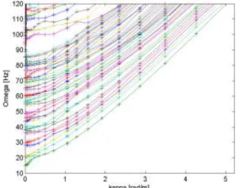
j 0 (10)First order correction for the imaginary part of the dynamic stiffness is then used to obtain a reduced model for which the frequency response can be computed efficiently. The second interest of computing periodic modes is to build a dispersion diagram showing the evolution of modal frequencies as a function of wavenumber.This motivates a strategy for choosing wave numbers. Instead of taking values evenly distributed in [0 2π] interval (which is the classic approach of discrete Fourier transform), the choice is made to refine the interval for small values of κ, and then to space the values as κ increases. This choice is justified looking at the shape of dispersion diagrams, for instance in Figure1 which represents dispersion diagram for the Carregado site (Alves Costa et al. 2012) described in section 3.
3. Results
The methodology described before is used to compute the results of a receptance test. The receptance of the track is the transfer function, obtained with an impact load of a hammer, between displacement and force at the loading point (Figure 2). This test is used to characterize track behavior in dynamics for a specified range of frequencies (De Man, 2002).
Figure 2: Hammer impact on rail, from (Verbraken et al.,2011)
3.1 Model description
A slice of track comprising rail, pad, sleeper, ballast, subballast, embankment and soil is modeled using finite elements and an Euler beam for rail.
The properties used for calculation are taken from (Alves Costa et al. 2012) and listed in Table 1. As soil is modeled as a semi-infinite half-space in the reference paper, an approximation is made for the presented calculation: 4 m of soil at 80 MPa are taken into account.
Table 1.Properties of the Carregado site
Layer Depth
(m)
Young Modulus (MPa)
Poisson ratio Density (kg/m3) Damping Ballast 0.22 97 0.12 1590 0.061 Subballast 0.35 212 0.20 1910 0.054 Embankment 0.30 212 0.20 1910 0.054 Soil 4 80 0.2 1900 0.06
Then, the methodology exposed in section 2 is applied to this slice in order to compute the frequency response of the track due to a hammer impact.
3.2 Comparison to a 2.5D FEM/BEM model
Using the methodology described in the previous section, a comparison with a receptance curve computed in paper (Alves Costa et al. 2012) with a 2.5D FEM/BEM model for the site of Carregado is led.
Figure 3: Comparison between receptance curves (a) from (Alves Costa et al., 2012) and (b) computed using the methodology described above
Both curves, displayed in Figure 3, present two main peaks, the first one is at 9 Hz in the reference model and around 20 Hz on the compared one, and the second peak at an higher frequency: 80 Hz for the reference graph and around 110 Hz for the present model. The first peak corresponds to a full vertical resonance of track, as displayed in Figure 4 a) (colors correspond to vertical displacement). The second peak is also mainly a vertical resonance of track, but other modes are contributing, as can be seen in the dispersion diagram in Figure 1.
a) b)
Figure 4 : Vertical displacement of track at the peak frequencies of Figure 3( a) at the first peak at 28 Hz and b) at the second peak at 113 Hz)
Regarding the response level, it is twice in the current model (Figure 3b) due to a unit force applied on rail, whereas in the reference curve (Figure 3a), only a half unit force is applied on each rail head.
As the shape of the two curves is similar, it is interesting to analyze causes of the differences in the peaks positions. As the reference model uses a BEM methodology, the
finite dimension of soil in the model presented here appears as the more evident explanation for these differences.
3.3 Impact of boundary conditions on receptance curve
Thus, in this paragraph the impact of the boundary conditions on the receptance curve is evaluated.
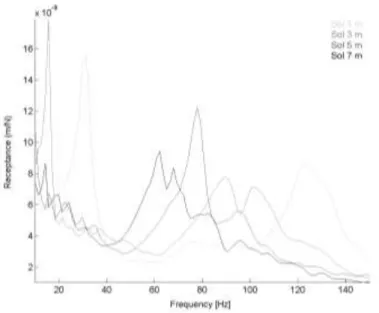
The first study is on lateral boundaries. In the 2.5D FEM/BEM model, there is no lateral boundary on soil, as it is modeled as an infinite half-space. In the initial mesh, the width of soil was taken equal to the embankment width given in the paper (Alves Costa et al. 2012): 7m. Figure 5 presents the evolution of the receptance curve when the width of soil increases, adding 1 m on each side up to 21 m.
As soil width increases, the second peak identified becomes more widespread, moves towards lower frequency and seems to converge around 90 Hz, which is close to the value of the reference model.
Figure 5: Comparison of receptance curves for different width of soil
Then the position of the lower boundary is studied. Receptance curves are computed for 1m of soil, 3m, 5m and 7m, all other parameters being constant.
Increasing the thickness of the soil layer considered leads to a shift of both principal peaks towards lower frequencies without convergence towards a set frequency. However, in a real track there is a peak characteristic of full track resonance between 40 and 140 Hz (Knothe and Grassie, 1993), and considering an homogenous layer of soil does not lead to a convergence towards such a peak.
3.3 Use of a non-linear elastic law for soil
The shift of the peaks to lower frequencies for increasing soil depths leads to question the considered soil model. To compute the curves of Figure 6, the soil has been taken as linear elastic, with a constant Young modulus for all depth. However, this modeling is an approximation as elastic soil modulus is rather increasing with confining pressure (Biarez and Hicher, 1994), and pressure is increasing with depth.Thus a more accurate rule will be taken into account :
zz yy yy zz n K and P ith P P E E 0 0 0 3 2 w (11)
In the soil layer, the elastic modulus will follow equation 11, E0 being a parameter to
adjust the elastic modulus to a known value at a given depth (for instance 120 MPa at 1 m of soil is taken below). P0 will be taken equal to atmospheric pressure. The exponent n
depends on the type of soil considered. For sands it will be equal to 0.4/0.5, for clays it will be higher, between 0.7 and 0.9 (Biarez and Hicher, 1994). In this case, the soil is mainly composed of sand, and the value of 0.5 is chosen. The earth pressure coefficient K0 is
taken equal to 0.5, leading to P=ρgh.
In Figure 7, the evolution of soil modulus with depth following this law is displayed.
Figure 7: Evolution of elastic modulus of soil with depth
The two peaks of the receptance curves correspond to the two first eigen frequencies of a column of soil, similar to that shown in Figure 7, having the same material properties as the railway track.
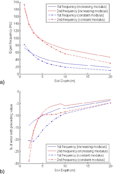
Following the evolution of these two first vertical eigen frequencies is thus similar to follow the evolution of the two peaks of the receptance curve. Figure 8 compares the evolution of these two frequencies for a soil modeled as an elastic linear homogenous media and as a non homogenous media, its elastic modulus following equation 11.
a)
b)
Figure 8: Evolution of the two first eigen frequencies with the thickness of soil layer (with dots for a contant modulus, without dots for an increasing modulus following Equation 11) Employing this law reduces the error made by approximating the soil by a finite layer, as displayed in Figure 8b). The lower part of the soil layer moves less in the second mode than in the first one, that can explain why stabilization of second frequency is faster than that of the first one. That can also explain why the error in Figure 8b) is rapidly lower for this second frequency than for the first one.Then, an optimal depth of soil can be found regarding error on both eigen frequencies. In the present case, the value of 10 m of soil seems a good choice as errors made on the first and second frequencies are lower than 10 % compared to the frequencies obtained with one additional meter of soil.
4. Conclusion
Two main conclusions can be drawn from this study. First, a competitive model has been proposed to compute the railway track response in the frequency domain. A further step will be to use this model in the time domain to compute the track response at a moving load.
Secondly, the soil characteristics have a great influence on the receptance curve, as shown in Figure 6: the depth of a bedrock, or the presence of a stiffer layer can easily be detected looking at the position of the two first peaks of the receptance curve, mostly influenced by the platform properties. Comparing receptance curves on a section of track
could then be a tool to detect changes in the substructure. A test campaign will be led on transition zones on the High Speed Line between Paris and Strasbourg (Costa D'Aguiar et al., 2013) to validate this statement and to exploit this testing.
5. References
Alves Costa, P., R. Calçada, & A. Silva Cardoso (2012). Ballast mats for the reduction of railway traffic vibrations. Numerical study.Soil Dynamics and Earthquake Engineering 42, 137–150.
Balmes, E. (2004-2013). http://www.sdtools.com/pdf/visc.pdf, Viscoelastic vibrationtoolbox, User Manual.
Biarez, J., &Hicher, P. Y. (1994). Elementary mechanics of soil behaviour: saturated
remoulded soils. AA Balkema.
Chebli, H., Othman, R., & Clouteau, D. (2006).Response of periodic structures due to moving loads. Comptes Rendus Mécanique, 334(6), 347-352.
Costa D'Aguiar S., Arlaud E.,Potvin R., Laurans E., Funfschillling C. (2013). Railway transitional zones: The challenges of very high speeds, Proceedings, World Congress
on Railway Research.
Degrande, G., &Schillemans, L. (2001). Free field vibrations during the passage of a Thalys high-speed train at variable speed. Journal of Sound and Vibration, 247(1), 144.
François, S., Schevenels, M., Galvín, P., Lombaert, G., &Degrande, G. (2010). A 2.5 D coupled FE–BE methodology for the dynamic interaction between longitudinally
invariant structures and a layered halfspace. Computer methods in applied mechanics
and engineering, 199(23), 1536-1548.
A. P. De Man. (2002). Dynatrack: A survey of dynamic railway track properties and their
quality.Phd, Delft University.
Knothe, K. L., &Grassie, S. L. (1993).Modelling of railway track and vehicle/track interaction at high frequencies.Vehicle system dynamics, 22(3-4), 209-262.
Knothe, K., & Wu, Y. (1998).Receptance behaviour of railway track and subgrade. Archive
of Applied Mechanics, 68(7-8), 457-470.
Lombaert, G., Degrande, G., Kogut, J., & François, S. (2006). The experimental validation of a numerical model for the prediction of railway induced vibrations. Journal of Sound
and Vibration, 297(3), 512-535.
Sheng, X., Jones, C. J. C., & Thompson, D. J. (2006).Prediction of ground vibration from trains using the wavenumber finite and boundary element methods.Journal of Sound
and Vibration, 293(3), 575-586.
Sternchüss, A. (2009). Multi-level parametric reduced models of rotating bladed disk
assemblies. Phd, Ecole Centrale Paris.
Verbraken H., Degrande G., Lombaert G., Stallaert B., Cuellar V. (2013). Benchmark testsfor soil properties, including recommendations for standards and guidelines.
Project no.scp0-ga-2010-265754 rivas, RIVAS D1.11.
Yang, Y. B., Hung, H. H., & Chang, D. W. (2003). Train-induced wave propagation in layered soils using finite/infinite element simulation. Soil Dynamics and Earthquake