A NURBS-BASED TOPOLOGY OPTIMIZATION METHOD INCLUDING ADDITIVE MANUFACTURING CONSTRAINTS

This is an author-deposited version published in: https://sam.ensam.eu

Handle ID: .http://hdl.handle.net/10985/12539

To cite this version :

Giulio COSTA, Marco MONTEMURRO, Jérôme PAILHES - A NURBS-BASED TOPOLOGY OPTIMIZATION METHOD INCLUDING ADDITIVE MANUFACTURING CONSTRAINTS - In: 7th International Conference on Mechanics and Materials in Design, Portugal, 20170611

PAPER REF: 6793

A NURBS-BASED TOPOLOGY OPTIMISATION METHOD

INCLUDING ADDITIVE MANUFACTURING CONSTRAINTS

Arts et Métiers ParisTech, I2M CNRS UMR 5295, F-33400, Talence, France

(*)_{Email: Giulio.Costa@ensam.eu}

ABSTRACT

In this work, the Solid Isotropic Material with Penalisation (SIMP) topology optimisation (TO) method for 2D structures is revisited and reformulated within the mathematical framework of Non-Uniform Rational BSpline (NURBS) functions. This implies several advantages: firstly, a NURBS surface allows for exploiting an implicitly defined filter zone; secondly, the number of optimisation variables (i.e. the parameters defining the NURBS surface) is relatively small when compared to the classical SIMP approach. Finally, the TO can be carried out by including linearity (either geometric or material) or non-conventional manufacturing constraints, as those related to the Additive Manufacturing (AM) technology. In this work, the TO is applied to a standard benchmark problem.

Keywords: NURBS, Topology Optimisation, Additive Manufacturing, SIMP.

INTRODUCTION

Topology Optimisation (TO) is a well-known design tool that provides extremely efficient mechanical structures. Often, the mathematical optimum solution could involve a really complicated geometry and topology: in some cases the optimised components cannot be fabricated through standard technologies. Nowadays, Additive Manufacturing (AM) seems to show all the requirements to achieve really optimised and manufacturable components both in plastics and in metal alloys (Guo and Leu, 2013). In spite of its great potential, AM has many difficulties to spread out in the industrial world. Moreover, only a little percentage of AM production is dedicated to functional parts which do not need post-treatment. In fact, there are two keys factors preventing the link between TO and effective AM techniques. On the one hand, there is a lack of consistency between the optimised geometries produced by TO commercial software and effective geometries that are reassembled after TO analysis in standard format file, as “.stp”, “.igs” or “.stl”. In particular, when one of the aforementioned files is imported in other FEM or CAD software, a lot of time is spent to obtain a connected and consistent geometry. On the other hand, despite its dimensional freedom, AM has intrinsic technological constraints which should be taken into account within TO analysis and not within a post-processing phase. Considering manufacturability constraints after the optimisation could seriously spoil the optimum solution and make the previous work useless (Mirzendehdel and Suresh, 2016). Some AM constraints have already been considered in the framework of TO, since they were conceived as further development of TO algorithms. Particularly, in the context of the SIMP method, the minimal member size is a typical constraint in TO (Poulsen, 2003): this requirement is fundamental for AM structures because it is related to the minimal printable dimension. A maximum member size constraint has been developed as well (Guest, 2009): it is estimated by means of a projection method.

Nevertheless, there are other constraints that need to be integrated within the TO algorithm when AM is chosen as manufacturing process. The first one concerns the orientation angle of the local tangent vector at the boundary surface: when the tangent vector overcomes a critical angle with respect to the manufacturing direction, a support structure is required. This limitation has been recognised and checked in several AM processes, such as Selective Laser Melting (SLM) and Electron Beam Melting (EBM) and it has been widely characterised (Kranz et al., 2015). Even if supports represent one of the most important constraint in a TO method finalised to AM, it is not the only one. It is evident that further constraints capable of taking into account thermal effects and residual stresses, typical of AM, are required.

In this paper, an innovative TO methodology for 2D structures is proposed in order to overcome the aforementioned drawbacks and to get solutions that are designed for AM. The well-known SIMP method is modified by relating the fictitious density (or pseudo-density) field 𝜌(𝐱) ∈ [0,1] to a suitable NURBS surface 𝜑(𝐱) (Piegl and Tiller, 1997), where 𝐱 is the position vector in the reference domain. Instead of assuming an unknown pseudo-density for each element of the underlying mesh, the number of variables is now defined by the value of the pseudo-density for each control point of the NURBS surface. Inspired by the idea of (Qian, 2013), when relating the SIMP density field to a suitable NURBS surface, many advantages occur: the first one is linked to the implicit filter zone that is defined by the blending functions local support. The size of such a filter zone depends on the degrees of the NURBS basis functions and on the knot vectors length (so it implicitly depends on the number of control points). As consequence, artefacts typical of the SIMP method, such as the “checkerboard effect”, as well as the mesh dependency are automatically overcome without establishing further filters. It is also interesting to remark how the implicit filter size (related to the NURBS formalism) affects the minimum length of features in TO. The present work goes beyond the analysis done by (Qian, 2013): the proposed strategy focuses on the design advantages, which can be got when the SIMP method is reformulated in the NURBS mathematical framework. Firstly, it will be shown that, in the context of the classical TO benchmark problem dealing with the compliance minimisation subject to an imposed volume fraction (an equality optimisation constraint), the solutions exhibit clearly defined bounds. Volume constraints are met both in the TO process and in the post processing phase, where the resulting optimised geometry is handled by external software. Moreover, the reconstruction phase for 2D structures is a completely automatic process: when the pseudo-density distribution is expressed through a NURBS surface, the boundary reconstruction is a straightforward step. Another significant advantage is the independence of the design variables (i.e. the value of the pseudo-density at each control point of the NURBS surface) from the elements of the predefined mesh. Finally, the NURBS-based approach allows a mathematically well-defined description of the boundaries in terms of both local normal vector and local curvature radius, so it is possible to impose constraints of different nature, especially those concerning the AM. Such an unconventional constraint on the curvature radius could enable the designer to manage both the smoothness of the boundaries and, indirectly, stress concentrations, which are typical in AM technologies.

The paper is structured as follows: in the second paragraph, the theoretical framework of the NURBS surfaces theory is briefly described. Then, in the third section the classic SIMP method is enhanced by means of the NURBS and the TO problem is stated as a constrained non-linear programming problem (CNLPP). The adopted numerical method is detailed in paragraph four. Section five illustrates a meaningful benchmark: in this background, the influence of the parameters defining the NURBS surface (number of control points, degrees

of the surface) has been investigated. The sixth paragraph concludes this article with some critical discussion and remarkable future perspectives.

THEORETICAL FRAMEWORK OF NURBS SURFACES

In this section, the fundamentals of the NURBS surfaces theory are briefly recalled. It is noteworthy that, since only 2D problems are considered, a NURBS surface suffices to obtain a suitable representation of the density field as function of the spatial coordinates 𝑥 and 𝑦 defined over the design space.

According to the notation of (Piegl and Tiller, 1997), a NURBS surface is defined as follows: 𝐒(𝑢, 𝑣) = ∑ ∑ 𝑅_𝑖,𝑗(𝑢, 𝑣)𝐏𝑖,𝑗 𝑛𝑣 𝑗=0 𝑛𝑢 𝑖=0 , (1)

where 𝑅_𝑖,𝑗(𝑢, 𝑣) are the piecewise rational basis functions, which are related to the standard NURBS blending functions 𝑁_𝑖,𝑝(𝑢) and 𝑁𝑗,𝑞(𝑣) by means of the relationship

𝑅𝑖,𝑗(𝑢, 𝑣) =

𝑁𝑖,𝑝(𝑢)𝑁𝑗,𝑞(𝑣)𝑤𝑖,𝑗 ∑𝑛_𝑘=0𝑢 ∑𝑛_𝑙=0𝑣 𝑁_𝑘,𝑝(𝑢)𝑁𝑙,𝑞(𝑣)𝑤𝑘,𝑙

. (2)

In equations (1) and (2), 𝐒(𝑢, 𝑣) is a bivariate vector-valued piecewise rational function, (𝑢, 𝑣) are scalar dimensionless parameters both defined in the interval [0,1], 𝑝 and 𝑞 are the NURBS degrees along 𝑢-direction and 𝑣-direction, respectively. 𝑤𝑖,𝑗 are the weights and 𝐏_𝑖,𝑗 = {𝑥_𝑖,𝑗, 𝑦_𝑖,𝑗, 𝑧_𝑖,𝑗} the Cartesian coordinates of the control points, with 𝑖 ∈ [0, 𝑛_𝑢] and 𝑗 ∈ [0, 𝑛_𝑣]. The net of (𝑛_𝑢+ 1) × (𝑛_𝑣+ 1) control points constitute the so-called control net. The blending functions are defined recursively by means of the Bernstein polynomials:

𝑁𝑖,0(𝑢) = {_{0 otherwise,}1 if 𝑈𝑖 ≤ 𝑢 ≤ 𝑈𝑖+1, (3)

𝑁_𝑖,𝑝(𝑢) = 𝑢 − 𝑈𝑖

𝑈_𝑖+𝑝− 𝑈_𝑖𝑁𝑖,𝑝−1(𝑢) +

𝑈_𝑖+𝑝+1− 𝑢

𝑈_𝑖+𝑝+1− 𝑈_𝑖+1𝑁𝑖+1,𝑝−1(𝑢), (4) where 𝑈_𝑖 is the 𝑖 − 𝑡ℎ component of the following non-periodic non-uniform knot vector

𝐔 = {0, … ,0⏟ 𝑝+1

, 𝑈_𝑝+1, … , 𝑈_{𝑚𝑢−𝑝−1}, 1, … ,1⏟ 𝑝+1

}. (5)

It is noteworthy that the size of the knot vector is 𝑚𝑢+ 1,

𝑚_𝑢 = 𝑛_𝑢+ 𝑝 + 1. (6)

Analogously, the 𝑁_𝑗,𝑞(𝑣) are defined on the knot vector 𝐕, whose size is 𝑚𝑣: 𝐕 = {0, … ,0⏟

𝑞+1

, 𝑉_𝑞+1, … , 𝑉_{𝑚𝑣−𝑞−1}, 1, … ,1⏟ 𝑞+1

𝑚_𝑣 = 𝑛_𝑣+ 𝑞 + 1. (8) The knot vectors 𝐔 and 𝐕 are two non-decreasing sequences of real numbers that can be interpreted as two discrete collections of values of the dimensionless parameters 𝑢 and 𝑣. As the control points, also the knot vectors components form a net. One basic property of the blending functions is the local support property: 𝑁𝑖,𝑝(𝑢) = 0 if 𝑢 is outside the interval [𝑈_𝑖, 𝑈_𝑖+𝑝+1). Hence, it is evident that 𝑅_𝑖,𝑗(𝑢, 𝑣) = 0 if (𝑢, 𝑣) is outside the rectangle [𝑈_𝑖, 𝑈_𝑖+𝑝+1) × [𝑉_𝑗, 𝑉_𝑗+𝑞+1), i.e. the local support associated to the control point 𝐏_𝑖,𝑗. The local support property is of paramount importance to understand all the advantages of the NURBS formulation of the SIMP method in the context of TO. For a deeper insight in the NURBS theory, the reader is addressed to (Piegl and Tiller, 1997).

THE NURBS-BASED TOPOLOGY OPTIMISATION METHOD: MATHEMATICAL FORMULATION

The classic SIMP Method

The SIMP method is here briefly recalled for the minimum compliance problem subject to an equality constraint on the volume for a 2D problem (Bendsøe and Sigmund, 2004).

Let us consider a rectangular reference domain 𝐷 ∈ ℝ2 in a Cartesian orthogonal frame 𝑂(𝑥, 𝑦). Let 𝐷 be defined as

𝐷 = {(𝑥, 𝑦) ∈ ℝ2| 𝑥 ∈ [0, 𝑤], 𝑦 ∈ [0, ℎ]}. ₍₉₎ where 𝑤 and ℎ are two reference lengths of the domain (that can vary depending to the considered problem) along x and y axes, respectively. The goal is to find the optimal distribution of a given isotropic material on 𝐷 by minimising the compliance (i.e. the virtual work of external applied loads) with an imposed volume fraction 𝑓 of the design domain. The material distribution (void and material zones) affects the stiffness tensor 𝐸_{𝑖𝑗𝑘𝑙}(𝐱), which is variable over the domain 𝐷. Let 𝛺 ⊆ 𝐷 be the material domain. In the SIMP approach the material domain is determined by means of a fictitious density function 𝜌(𝐱) ∈ [0,1] defined over the whole design domain 𝐷. Such a density field is related to the material distribution and, accordingly, to the local stiffness tensor. 𝜌(𝐱) = 0 means absence of material, whilst 𝜌(𝐱) = 1 implies completely dense base material. The dependence of the stiffness tensor 𝐸_{𝑖𝑗𝑘𝑙}(𝜌(𝐱)) on the density field 𝜌(𝐱) is provided by

𝐸_{𝑖𝑗𝑘𝑙}(𝜌(𝐱)) = 𝜌(𝐱)𝛼_𝐸

𝑖𝑗𝑘𝑙0 , (10)

where 𝐸_{𝑖𝑗𝑘𝑙}0 is the stiffness tensor of the isotropic material and 𝛼 ≥ 3 a suitable parameter that aims at penalising all the meaningless densities between 0 and 1. Let 𝐮 be the displacement vector field and 𝑙(𝐮) the compliance of the structure. During the optimisation process, the equilibrium equation is implicitly imposed in its weak form:

𝑙(𝐮) = ∫ 𝜌(𝐱)𝛼𝐸_{𝑖𝑗𝑘𝑙}0 𝜀𝑖𝑗(𝐮)𝜀𝑘𝑙(𝐯) 𝑑𝐷 𝐷

. (11)

In equation (11), 𝐯 is a kinematic admissible displacement vector, 𝜀𝑖𝑗 is the linear strain tensor. In order to prevent any singularity of the equilibrium problem, a lower non-null

boundary is applied to the density field, so 𝜌(𝐱) ∈ [𝜌𝑚𝑖𝑛, 1], with usually 𝜌𝑚𝑖𝑛 = 10−3. Then, the mathematical formulation of the TO problem is given by:

min𝜌(𝐱)𝑙(𝐮), subject to { 𝑉(𝐱) 𝑉𝑡𝑜𝑡 =∫ 𝜌(𝐱) 𝑑𝐷𝐷 ∫ 𝑑𝐷_𝐷 = 𝑓, 0 < 𝜌𝑚𝑖𝑛 ≤ 𝜌(𝐱) ≤ 1. (12)

Classically, such a problem can be solved by a suitable gradient-based algorithm coupled to a FEM solver. The variables of problem (12) are the pseudo-densities computed at the centroid of each element (𝜌_𝑒) constituting the mesh. Hence, the FEM-discretised version of problem (12) writes

min_𝜌𝑒{𝐅} ∙ {𝐔FEM} = min 𝜌𝑒 𝑐(𝜌_𝑒), subject to { (∑ 𝜌_𝑒𝛼[𝐊_𝐞] 𝑁𝑒 𝑒=1 ) {𝐔_𝐅𝐄𝐌} = {𝐅} 𝑉(𝜌_𝑒) 𝑉_𝑡𝑜𝑡 = ∑𝑁𝑒 𝜌_𝑒 𝑣_𝑒 𝑒=1 𝑁_𝑒𝑣_𝑒 = 𝑓, 0 < 𝜌_𝑚𝑖𝑛 ≤ 𝜌_𝑒 ≤ 1, 𝑒 = 1, … , 𝑁_𝑒, (13)

where {𝐅} and {𝐔_FEM} are, respectively, the vector of nodal generalised forces and displacements in the global reference system while [𝐊_𝐞] is the element stiffness matrix expanded over the full set of degrees of freedom (DOFs) of the structure. It must be pointed out that the SIMP method can lead to numerical issues, e.g. the well-known “checkerboard effect”, which are due to the lack of mutual dependency among the design variables. To repair these issues, a distance-based filter is usually employed (Bendsøe and Sigmund, 2004).

The proposed NURBS-based SIMP method

In the framework of the proposed approach, the pseudo-density field characterising the SIMP method is related to a suitable NURBS scalar function. In the following, only Bspline functions have been employed for sake of simplicity, thus all the weights in equation (2) are equal to 1.

In the context of Bspline functions, the pseudo-density field writes: 𝜌(𝑢, 𝑣) = ∑ ∑ 𝑁𝑖,𝑝(𝑢)𝑁𝑗,𝑞(𝑣)𝜌̅𝑖,𝑗 𝑛𝑣 𝑗=0 𝑛𝑢 𝑖=0 . ₍₁₄₎

The shape of the Bspline is affected by the value of the pseudo-density at each control point, i.e. 𝜌̅_𝑖,𝑗, as well as by the value of the other parameters involved into the definition of the Bspline scalar function, namely the degrees of the blending function, i.e. p and q, the number

of control points (related to the parameters 𝑛_𝑢 and 𝑛_𝑣) and the value of the knot vectors components, as illustrated in Eqs. (2) and (4). The dimensionless parameters 𝑢 and 𝑣 shown in Eq. (14) are related to the Cartesian coordinates of the global frame as:

𝑢 = 𝑥 𝑤, 𝑣 =𝑦

ℎ.

(15)

In equation (14) 𝜌̅_𝑖,𝑗 are the design variables of the NURBS-based SIMP method. They are collected in a column array 𝛏 and suitable boundaries are imposed to satisfy the density field requirements for the TO problem:

𝛏𝐭= {𝜌̅̅̅̅̅, … , 𝜌_0,0 ̅̅̅̅̅̅̅ 𝜌_𝑛𝑢,0,̅̅̅̅̅ … , , 𝜌_0,1 ̅̅̅̅̅̅, … , 𝜌_𝑛𝑢,1 ̅̅̅̅̅̅, 𝜌_0,𝑛𝑣 ̅̅̅̅̅̅̅̅}, _{𝑛𝑢,𝑛𝑣} 𝜌𝑖,𝑗

̅̅̅̅ ∈ [10−3, 1] ∀𝑖 = 0, … , 𝑛𝑢, ∀𝑗 = 0, … , 𝑛𝑣.

(16) Without loss of generality, in this work the two knots vector 𝐔 and 𝐕 are considered uniformly distributed in the interval [0,1] and both the degrees of the blending functions and the number of control points are fixed a priori.

In this background the TO problem can be stated (for the 2D case) as follow: min𝛏𝑙(𝛏), subject to: { 𝐸𝑖𝑗𝑘𝑙(𝜌(𝛏)) = 𝜌(𝛏)𝛼𝐸𝑖𝑗𝑘𝑙0 , 𝑉(𝛏) 𝑉_𝑡𝑜𝑡 = ∫ ∫ 𝜌(𝛏) 𝑑𝑥𝑑𝑦₀𝑤 ₀ℎ 𝑤ℎ = 𝑓, 𝐠(𝛏) ≤ 𝟎, 𝜉𝑘 ∈ [10−3, 1] ∀𝑘 = 1, … , (𝑛𝑢+ 1) × (𝑛𝑣+ 1). (17)

In problem (17), 𝐠(𝛏) is the vector collecting the technological constraints related to the considered AM process.

The FEM discretised version of problem (17) is

min_𝛏{𝐅} ∙ {𝐔FEM} = min_𝛏 𝑐(𝜌(𝛏)), subject to { (∑ 𝜌_𝑒𝛼[𝐊_𝐞] 𝑁𝑒 𝑒=1 ) = [𝐊], 𝑉(𝜌_𝑒) 𝑉_𝑡𝑜𝑡 = ∑𝑁𝑒 𝜌_𝑒 𝑒=1 𝑒_𝑥𝑒_𝑦 = 𝑓, {𝐠(𝛏)} ≤ {𝟎}, 𝜉_𝑘 ∈ [10−3, 1] ∀𝑘 = 1, … , (𝑛_𝑢+ 1) × (𝑛_𝑣+ 1). (18)

𝜌_𝑒 = 𝜌(𝑢_𝑒, 𝑣_𝑒) = 𝜌 (𝑥𝑒 𝑤,

𝑦𝑒

ℎ), (19)

where (𝑥_𝑒, 𝑦_𝑒) are the Cartesian coordinates of the element centroid, whilst [𝐊] is the global stiffness matrix and 𝑒𝑥 and 𝑒𝑦 are the number of mesh divisions along 𝑥 and 𝑦 axes, respectively.

The SIMP approach revisited in the NURBS mathematical framework is characterised by a given number of features which implies just as many advantages:

1) the number of design variables is unrelated to the number of elements. In the classic SIMP approach, each element introduces a new design variable. In the NURBS framework, the accuracy of the topology description is characterised solely by the number of points of the control net, i.e. (𝑛_𝑢+ 1) × (𝑛_𝑣 + 1);

2) the locally supported blending functions imply an implicitly defined filter zone. The size of such a filter zone is related to the dimensions of the local support of the blending functions. It should be remarked that standard TO filters create a mutual dependency area among the elements densities, i.e. the design variables. In the case of the NURBS, the inter-dependence is automatically provided between the NURBS control points, without the need of defining a filter on the mesh elements densities. 3) the NURBS formalism allows taking into account new kinds of constraints, since a

mathematically well-defined description of the geometrical bounds of the optimum topology is always available during the iterations of the optimisation process.

In the following, the mathematical formulation and the implementation of a suitable constraint on the radius of curvature is briefly discussed: this is only an example to prove the effectiveness of the proposed approach. More sophisticated, AM-oriented, technological constraints are forecast for the immediate future.

The curvature radius constraint

The quality of the boundaries of the optimum topology of a given product is of paramount importance for both manufacturing and mechanical viewpoints: regions characterised by a small local curvature radius should be avoided in order to limit stress concentration. To this purpose, in this work a mathematical formalisation of the curvature radius constraint is introduced in the framework of the NURBS-based SIMP approach.

In the classical SIMP method, the first issue to be faced is the absence of a mathematical representation of the boundary of the structure during the optimisation process. Indeed, in the context of the SIMP method the boundary is determined at the end of the TO by interpolation of the nodes of the retained elements after convergence. Conversely, in the framework of the NURBS formalism, a mathematical description of the boundaries is available by establishing a proper cutting plane for the Bspline (during the iterations). Let 𝛺 ⊆ 𝐷 be the material domain and 𝜌_𝑐𝑢𝑡 ∈ [10−3_{, 1] the threshold cutting value for the density field. Since the} pseudo-density field is given by the NURBS scalar function of Eq. (14), the relationship

𝜌𝑐𝑢𝑡− 𝜌(𝛏) = 0 (20)

implicitly provides the boundary of the structure. In particular, a given point belongs to (or is out of) the material domain 𝛺 if the following conditions are met:

{

(𝑥, 𝑦) ∈ 𝛺, 𝑖𝑓 𝜌(𝛏) > 𝜌𝑐𝑢𝑡, (𝑥, 𝑦) ∈ 𝜕𝛺, 𝑖𝑓 𝜌(𝛏) = 𝜌_{𝑐𝑢𝑡,}, (𝑥, 𝑦) ∈ 𝐷|𝛺, 𝑖𝑓 𝜌(𝛏) < 𝜌𝑐𝑢𝑡.

(21) For an implicitly defined curve, the equation of the curvature is available in (Goldman, 2005) and writes 𝜒 = {𝜕𝜌_𝜕𝑦 −𝜕𝜌_𝜕𝑥} [ 𝜕2𝜌 𝜕𝑥2 𝜕2𝜌 𝜕𝑥𝜕𝑦 𝜕2𝜌 𝜕𝑥𝜕𝑦 𝜕2𝜌 𝜕𝑦2 ] { 𝜕𝜌 𝜕𝑦 −𝜕𝜌_𝜕𝑥 } [(𝜕𝜌_𝜕𝑥) 2 + (𝜕𝜌_𝜕𝑦) 2 ] 3 2 . (22)

Thanks to the NURBS formalism the derivatives of the pseudo-density can be easily computed in a recursive manner, see (Piegl and Tiller, 1997). Considering the composed derivative, the curvature radius (that is the reciprocal value of the curvature) writes

𝑅 = 1 𝑤ℎ [ℎ2(_𝜕𝑢𝜕𝜌) 2 + 𝑤2(𝜕𝜌_𝜕𝑣) 2 ] 3 2 (𝜕𝜌_𝜕𝑢) 2 𝜕2_𝜌 𝜕𝑣2− 𝜕𝜌 𝜕𝑢 𝜕𝜌 𝜕𝑣 𝜕2_𝜌 𝜕𝑢𝜕𝑣+ ( 𝜕𝜌 𝜕𝑣) 2 𝜕2_𝜌 𝜕𝑢2 . (23)

To be remarked that in Eqs. (22) and (23) the dependence on both the coordinates (𝑥, 𝑦) and the design variable array 𝛏 has been omitted for sake of simplicity.

Therefore, the constraint on the admissible value of the local radius of curvature can be formalised as:

𝑔(𝛏) = 𝑅̅ − min

𝜕𝛺 |𝑅(𝑥, 𝑦)| ≤ 0, (24)

where 𝑅̅ represents the minimum admissible value for the curvature radius for the considered application.

NUMERICAL STRATEGY

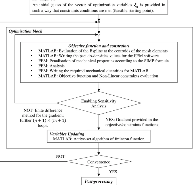
In this section a suitable numerical strategy for solving the CNLPP (18) is presented. A synthetic scheme of the numerical strategy is illustrated in Figure 1:. Only few comments are added in order to clarify the procedure.

Pre-processing: both a mesh and a NURBS parametrisation are associated to the geometrical

reference domain. The boundary conditions and loads are set. The user can enable a symmetric solution (i.e. a symmetric shape of the Bspline scalar function defining the pseudo-density). At this stage the user has to set the objective function as well as the optimisation constraints for the problem at hand.

Initialisation: for a given problem usually the pseudo-density field is initialised in order to

satisfy the volume constraint at the beginning of the optimisation.

Optimisation Block: it should be remarked that sensitivity analysis is not automatically

activated; some problems have simple objective and constraints functions, so derivatives can be easily provided in analytical form. However, the algorithm, in its most general form, does

not require the gradient provision and it can be adequate for whatever customised problem. Of course, this would penalise computational time.

Figure 1: The numerical strategy – synthetic scheme.

Optimisation block

Objective function and constraints

• MATLAB: Evaluation of the Bspline at the centroids of the mesh elements • MATLAB: Writing the pseudo-densities values for the FEM software • FEM: Penalisation of mechanical properties according to the SIMP formula • FEM: Analysis

• FEM: Writing the required mechanical quantities for MATLAB • MATLAB: Objective function and Non-Linear constraints evaluation

Enabling Sensitivity Analysis

Pre-processing

• Bspline parameterisation

• Mesh, Loads, Boundary Conditions (BC) • Choice of constraints and objective function • Enabling Symmetries

• Enabling Sensitivity analysis

Initialization

An initial guess of the vector of optimization variables 𝝃_𝟎 is provided in such a way that constraints conditions are met (feasible starting point).

NOT: finite difference method for the gradient: further (𝑛 + 1) × (𝑚 + 1)

loops.

Variables Updating

MATLAB: Active-set algorithm of fmincon function

YES: Gradient provided in the objective/constraints functions

Convergence YES NOT

RESULTS

In order to prove the effectiveness of the proposed approach several benchmarks and real-world engineering problems have been analysed. However, for the sake of brevity, in this section only some meaningful results related to the “cantilever plate” benchmark illustrated in Figure 2 are discussed. The results including the technological constraint on the local radius

of curvature (together with other meaningful benchmarks) will be presented in an extended version of this manuscript.

The aim is to minimise the compliance by keeping the volume of the structure at the 40% of the starting volume. All geometrical and mechanical data are provided in the caption of Figure 2.

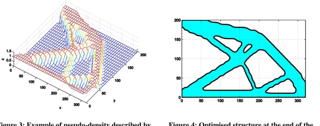
Figure 3 shows a typical result of the TO analysis: the pseudo-density NURBS function. The corresponding optimised structure is depicted in Figure 4 and it is obtained by means of the intersection of the aforementioned NURBS with a suitable cutting plane. For all the considered benchmarks, the compliance is evaluated after cutting the Bspline surface with the cutting plane and compared with the value provided by the TO algorithm at the end of the analysis. This comparison (in terms of objective function values) is considered in order to prove the consistency of the proposed method.

Figure 3: Example of pseudo-density described by means of a Bspline function

Figure 4: Optimised structure at the end of the NURBS-based TO method

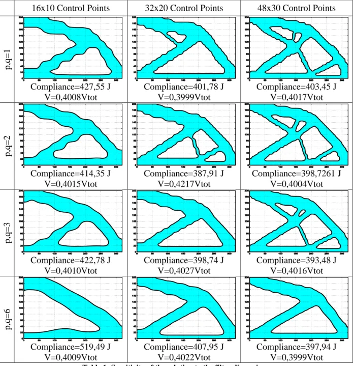
The first campaign of analyses aims at investigating the effects of the filter zone dimensions on the final topology. Being the filter zone affected by the discrete parameters of the NURBS, the following analyses have been performed by changing both the NURBS degrees and the Figure 2: The proposed benchmark – In-plane dimensions: w =320mm, h=200 mm. Thickness: t=2 mm.

number of control points. Results are collected in Table 1 in the case of a fixed mesh of 40 × 25 SHELL elements with 8 nodes and 6 degrees of freedom per node.

16x10 Control Points 32x20 Control Points 48x30 Control Points

p,q= 1 Compliance=427,55 J V=0,4008Vtot Compliance=401,78 J V=0,3999Vtot Compliance=403,45 J V=0,4017Vtot p,q= 2 Compliance=414,35 J V=0,4015Vtot Compliance=387,91 J V=0,4217Vtot Compliance=398,7261 J V=0,4004Vtot p,q= 3 Compliance=422,78 J V=0,4010Vtot Compliance=398,74 J V=0,4027Vtot Compliance=393,48 J V=0,4016Vtot p,q= 6 Compliance=519,49 J V=0,4009Vtot Compliance=407,95 J V=0,4022Vtot Compliance=397,94 J V=0,3999Vtot Table 1: Sensitivity of the solution to the filter dimensions

The dimensions of the filter increase when the degrees increase or when the number of control points decreases. So, evident changes in resulting topologies occur: when the number of control points increases the final optimum topology has better quality (together with better performances) and thinner features (i.e. thin branches) appear. Conversely, increasing the degrees implies an inhibition of such features. Hence, it is evident that the dimension of the filter zone affects the minimum member size that can be expected from the topology optimisation. It should be also highlighted that, if objective function values are compared, only the solution 𝑝, 𝑞 = 6 with 16 × 10 control points is significantly far from the other solutions: it can be explained by the fact that the filter dimensions are too big and the zone of interdependence among elements is too extended. So, the algorithm tends to converge on a

pseudo-optimal solution. However, increasing too much the number of control points or decreasing the degree of the blending functions does not imply a more efficient solution (in terms of both objective and constraint functions).

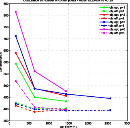
Figure 5: Objective function vs number of control points for a 40x25 mesh elements

Furthermore, too small filter dimensions lead to misleading results. When the filter dimensions are lower than or equal to those of the elements, the checkerboard effect appears also in the framework of the NURBS-based SIMP approach.

Concerning the volume equality constraint, it is strictly met in the examined configurations (after performing the geometrical reconstruction of the optimum topology). Indeed this is a strong advantage of the NURBS-based SIMP approach: when the pseudo-density field is described through a NURBS scalar function, it is automatically compatible with any standard format of data exchange (IGS, STEP, etc.) and the optimum topology can be easily transferred from the FE code to a CAD software without the need of any curve/surface fitting phase. Conversely, in the framework of the classical SIMP approach (where the volume constraint is met only in the element-discretised domain) there is not any ad-hoc rule to retrieve the boundary of the optimum topology by rigorously satisfying the volume constraint during CAD rebuilding phase (often the optimum topology is described through the positions of the elements nodes at the end of the analysis and requires complex surface and/or curve fitting operations which lead to a considerable increase of the volume of the final topology). Moreover, Figure 5 shows the trends of the compliance versus the number of control points for several values of the surface degrees. In this figure, the objective function at the end of the optimisation is called “obj opt” and it is the nominal compliance of the structure evaluated on the whole domain 𝐷 with a mapped mesh (it is represented with a continuous line). The

From an accurate analysis of results provided in Table 1 and Figure 5 two basic facts can be deduced:

 for each analysis the effective compliance is always smaller than the nominal one. This means that the proposed methodology is conservative (in terms of the strain energy of the structure);

 when the number of control points reaches a threshold value (when the number of control point is about the 75% of the mesh elements) it has no more influence on the value of the compliance. This means that even the user chooses of increasing the number of control points beyond this threshold there is almost any influence on the values of the objective/constraint functions. This fact also proves that the number of design variables is

unrelated to the mesh size and, if the aforementioned constraints on the filter dimensions

are met, the designer is free to choice the best compromise between computational time and accuracy in the description of the involved physical phenomena.

CONCLUSIONS

This study aims at proving the possibility of enhancing the classic SIMP approach in the context of the NURBS formalism for 2D structures. The main effects of such a choice have been investigated and the main results can be summarised as follows.

1) The NURBS representation of the pseudo-density introduces an implicitly defined filter zone that should be properly sized by means of the NURBS discrete parameters in order to avoid numerical artefacts or premature convergence on pseudo-optimal solutions. 2) If the dimensions of the filter are big enough (i.e. superior to the mesh characteristic

dimension) in order to prevent the checkerboard effect, there is a substantial independence of the resulting objective function from the number of the NURBS control points. Therefore, increasing the number of design variables beyond to a given threshold value (which depends upon the problem at hand) does not affect the result in terms of objective and constraint functions.

3) The final rebuilt structure (i.e. the CAD geometrical representation of the optimum topology) exhibits conservative and consistent properties in terms of both the objective function and the volume constraint: for the considered examples the CAD representation of the optimum solution has always the same (or a lower) objective function value (when compared to that provided by the TO algorithm) and exactly meets the volume constraint.

4) Using the NURBS allows for precisely describing the structure boundaries, so unconventional constraints related to the AM technology can be imposed. In this paper a constraint on the radius of curvature has been successfully included in the TO.

This work opens several perspectives: first of all, some constraint, typical of the AM technology, can be included in the TO. In this sense, the most important constraints to be taken into account are the minimum length scale size and the volume of support. The first constraint should be imposed on the true boundary of the structure and not on the mesh elements. Therefore, the minimum length constraint would exactly correspond to the actual minimum printable feature size. Concerning the latter constraint, it can be stated that the most efficient way to deal with support structures could be a minimisation of their volume rather than avoiding their presence on the final product. Finally, the most challenging perspective is to develop the NURBS-based SIMP approach in the most general 3D case.

ACKNOWLEDGMENTS

The first author is grateful to Nouvelle-Aquitaine region for supporting this research work through the FUTURPROD project.

REFERENCES

Bendsøe, M.P., Sigmund, O., 2004. Topology Optimization. Springer Berlin Heidelberg, Berlin, Heidelberg.

Goldman, R., 2005. Curvature formulas for implicit curves and surfaces. Computer Aided Geometric Design 22, 632–658.

Guest, J.K., 2009. Imposing maximum length scale in topology optimization. Structural and Multidisciplinary Optimization 37, 463–473.

Guo, N., Leu, M.C., 2013. Additive manufacturing: technology, applications and research needs. Frontiers of Mechanical Engineering 8, 215–243.

Kranz, J., Herzog, D., Emmelmann, C., 2015. Design guidelines for laser additive

manufacturing of lightweight structures in TiAl6V4. Journal of Laser Applications 27, S14001.

Mirzendehdel, A.M., Suresh, K., 2016. Support structure constrained topology optimization for additive manufacturing. Computer-Aided Design 81, 1–13.

Piegl L, Tiller W, The NURBS Book, Springer-Verlag, New York, 1997.

Poulsen, T.A., 2003. A new scheme for imposing a minimum length scale in topology optimization. International Journal for Numerical Methods in Engineering 57, 741– 760.

Qian, X., 2013. Topology optimization in B-spline space. Computer Methods in Applied Mechanics and Engineering 265, 15–35.