HAL Id: hal-00603639
https://hal.archives-ouvertes.fr/hal-00603639v2
Submitted on 20 Oct 2012
HAL is a multi-disciplinary open access
archive for the deposit and dissemination of
sci-entific research documents, whether they are
pub-lished or not. The documents may come from
teaching and research institutions in France or
abroad, or from public or private research centers.
L’archive ouverte pluridisciplinaire HAL, est
destinée au dépôt et à la diffusion de documents
scientifiques de niveau recherche, publiés ou non,
émanant des établissements d’enseignement et de
recherche français ou étrangers, des laboratoires
publics ou privés.
Hierarchical clustering for graph visualization
Stéphan Clémençon, Hector de Arazoza, Fabrice Rossi, Viet Chi Tran
To cite this version:
Stéphan Clémençon, Hector de Arazoza, Fabrice Rossi, Viet Chi Tran. Hierarchical clustering for
graph visualization. European Symposium on Artificial Neural Networks (ESANN 2011), Apr 2011,
Bruges, Belgium. pp.227-232. �hal-00603639v2�
Hierarchical clustering for graph visualization
St´ephan Cl´emen¸con1, Hector De Arazoza2, Fabrice Rossi1 and Viet-Chi Tran3∗
1- Institut T´el´ecom, T´el´ecom ParisTech, LTCI - UMR CNRS 5141 46, rue Barrault, 75013 Paris – France
2- Facultad de Matem´atica y Computaci´on, Universidad de la Habana, La Habana, Cuba
3- Laboratoire Paul Painlev´e UMR CNRS No. 8524, Universit´e Lille 1, 59 655 Villeneuve d’Ascq Cedex, France
Abstract. This paper describes a graph visualization methodology based on hierarchical maximal modularity clustering, with interactive and significant coarsening and refining possibilities. An application of this method to HIV epidemic analysis in Cuba is outlined.
1
Introduction
Large graphs and networks are natural mathematical models of interacting objects such as persons in social networks, articles in citation networks, etc. [8]. Unfortunately, the sizes of real networks strongly limit visual exploratory analysis of their properties. Indeed, despite the numerous graph visualization methods available [3, 7], displaying a graph with hundreds of vertices or more in a meaningful way remains difficult. It is therefore common to rely on simplification techniques to draw a summary of a complex graph: in general, a graph clustering algorithm is used to identify clusters of nodes and the graph induced by the clustering is drawn [4]. When the clustering is hierarchical, the full graph can be represented using the structure imposed by the hierarchy: the general layout is given by the higher level of the hierarchy in which the graph is strongly simplified, then details are added in a top down way by descending the hierarchy (see e.g., [1] for a recent algorithm of this type).
Those approaches generally consider the (hierarchical) clustering of the graph nodes to be obtained via one of the numerous graph clustering methods available [5, 13]. In addition, the significance of the hierarchical clustering is generally not questioned, while a bad clustering could lead to serious interpretation errors. We propose in this paper a methodology that addresses those two aspects.
2
Clustered graph construction
This section described the proposed methodology which consists in building a hierarchical graph clustering with guaranteed significance at each level, using maximal modularity clustering as a building block.
∗This work was supported by the French Agency for Research under grant ANR Viroscopy
2.1 Maximal modularity clustering
As show in recent surveys [5, 13], dozens of graph clustering methods have been proposed. However, as pointed out in e.g. [12], not all of them are adapted to graph visualization. In seems indeed important to obtain clusters of nodes with a high density of internal connections and a low number of external connections, i.e., to find what is frequently called communities. Among the corresponding clustering methods, the ones that maximize the modularity of the obtained partition seem the more adapted: modularity maximization has been shown to produce interesting partitions in many applications [5] and maximizing the modularity is equivalent [9], to some extend, to optimizing the energy models used in many graph visualization method, such as the standard Fruchterman Reingold algorithm [6].
While maximizing the modularity is a NP hard problem, high quality sub-optimal solutions can be obtained efficiently, for instance using deterministic annealing [12] or greedy methods such as [10]. Those latter methods have reasonable computational complexities, proportional to the number of edges in the graph multiply by the number of nodes: the implementation proposed in [10] can cluster a graph with 75 000 nodes and 120 000 edges in less than 2 minutes on standard PC hardware.
2.2 Clustering Significance
While modularity is normalized and takes values between −1 and 1, it is a priori difficult to tell whether a given value corresponds to an actual significant partition of the graph or is just a manifestation of random fluctuation. Indeed modularity maximization algorithms will generally discover some partition in a random graph with no cluster structure. As clustered graph visualization strongly relies on the hierarchical partitioning scheme, only significant partitions should be considered. This could be done with the help of theoretical results from [11]. Indeed, the authors compute the expected maximal modularity of random graphs with arbitrary degree distribution. Given a graph, one can apply those results to its empirical degree distribution to get a threshold value for the modularity; then if a clustering has a larger modularity, it is assumed to be significant, i.e., to represent a real structure in the graph.
This approach suffers from two drawbacks. Results from [11] are only asymp-totically valid in the limit of large and dense graphs. In addition, only the expected value is given, not the fluctuations around this value (e.g., the variance). We propose therefore to rely on a simpler monte carlo strategy. We built random graphs with no structure that have exactly the same degree distribution as the one of the graph under study (this is the configuration model random graph, see e.g., [8]). Then we apply a maximal modularity clustering algorithm (the one from [10]) to each of the random graph. The obtained distribution of the modularity is valid under the null hypothesis of no clustering and can be used to compute an estimate of the p-value of the modularity of the clustering obtained on the original graph. This procedure is time consuming, but current clustering
methods are efficient enough to allow it for medium scale graphs for e.g. 100 random trials. We recommend to consider the clustering significant only if no random graph lead to a modularity higher than the one of the original graph, i.e., for a p-value lower than 1%. For large scale graphs, we fall back to the approximation provided in [11].
2.3 Hierarchical clustering
To produce a clustered graph, we proceed as follows. We first compute a maximal modularity clustering of the full graph and assess its significance using the simulation strategy described above. If the clustering is not relevant, then no meaningful representation can be done: this is reported to the user as it means that the graph under study is better modelled as a random network without structure than via clustering.
Depending on the size of the graph and on the number of clusters produced by the clustering algorithm, more coarsening and/or more refinement might be useful. Following the general idea of clustered graph analysis, the clustering is refined on a per cluster basis: we apply the same clustering method to each of the clusters of the original graph, considered separately, that is discarding inter-cluster connections. This can be repeated recursively if needed, while keeping only significant clusterings. More precisely, two significance levels are checked. We first apply the methodology described above while considering the sub-graph in isolation. If the clustering is significant, we also test its impact when integrated in the global clustering of the graph: we make sure that, apart from the bottom level, each level of the hierarchy contains a significant clustering of the original graph.
Coarsening is done differently by applying the greedy strategy used by efficient modularity maximization algorithms, in its simplest form: cluster pairs that induce the least reduction in modularity are merged recursively as long as the modularity of the obtained clustering remains above the significance level.
3
Visualization
The visualization of the clustered graph is based on classical solutions, such as [1], with an important difference. Indeed, efficient modularity maximization algorithms use generally greedy coarsening techniques: any merge of the clusters of the best clustering will reduce the modularity. Therefore, using the highest level of the hierarchy to guide the display of the graph is likely to induce suboptimal visualization (based on results of [9]). Then we rely on the following strategy.
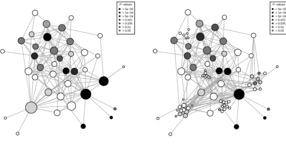
A variant of the Fruchterman Reingold (FR) algorithm [6] is used to layout the quotient graph with the best modularity: the repulsive force from a node is weighted by the size of cluster it represents, rather than being uniform. This resulting display is the original solution proposed to the user (see Figure 1 (a) for an example). Each node of this graph represents a cluster, while edges are added between clusters whose members are connected in the original graph. The surface of each node is proportional to the cluster size. Colors (or gray levels) can
P−values > 5e−05 > 1e−04 > 5e−04 > 0.001 > 0.005 > 0.01 > 0.05
(a) Best partition
P−values > 5e−05 > 1e−04 > 5e−04 > 0.001 > 0.005 > 0.01 > 0.05
(b) Maximally refined partition
Fig. 1: Clustered graph visualization
be used to encode cluster specific information, such as the internal connection density, or, as shown on Figures 1 and 2, to display quantities related to the distribution of some node property inside the cluster.
Then an interactive exploration is provided. The user can request the refining of the clustering. This is done by descending in the hierarchical partition, down to the last level that provide a significant clustering. At each refinement step, the layout of the previous level is used for non refined nodes, while the FR algorithm is applied to the refined node (see Figure 1 (b)).
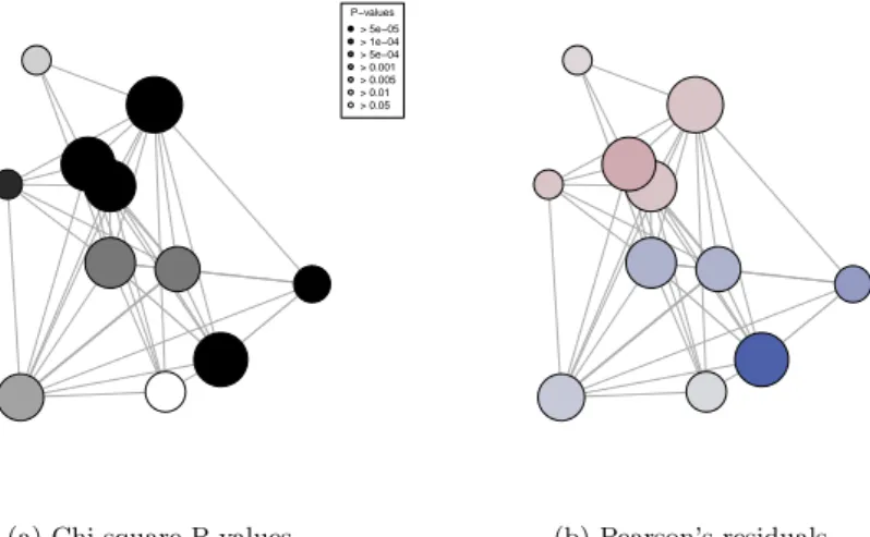
Coarsening is done in a similar but simpler way: the position of the node that replaces nodes merged from the previous level is obtained as the center of mass of those nodes, weighted by the size of the associated clusters (see Figure 2).
4
Application to the Cuban HIV-AIDS epidemic
The proposed methodology is used to explore the largest connected component of a graph of sexual contacts between patients infected by the HIV in Cuba (see [2] for details). The corresponding database has been obtained via the infection tracing methodology: when an individual is tested as HIV positive, she/he is asked to name her/his sexual partners in the last two years. The sexual contact is recorded for each partner already in the database. Others are contacted and proposed a diagnosis. Positive new cases are added to the database and the tracking proceeds. The database includes important information about the patients, including there sexual orientation, age at detection, etc. Up to 2006, the database contains almost 5 400 persons, among which 2 386 belong to a single connected component. Applied to the corresponding graph, classical visualization algorithms provide no insight on the epidemic.
Using [10], we obtain a partition of the graph into 39 clusters, with a modu-larity of 0.85. This is significantly higher than the modularities of random graphs
P−values > 5e−05 > 1e−04 > 5e−04 > 0.001 > 0.005 > 0.01 > 0.05
(a) Chi square P values (b) Pearson’s residuals
Fig. 2: Coarsened clustered graph visualization
with identical sizes and degree distributions: the highest value among 50 random graphs is 0.74. The corresponding layout is given by Figure 1 (a): in this display nodes are darkened according to the p-value of a chi-squared test conducted on the distribution of the sexual orientation of persons in each cluster versus the distribution of the same variable in the full connected component. It appears clearly that some clusters have a specific distribution of the sexual orientation variable.
The possibility of refining the clustering in this case is quite limited: only 5 of the 39 clusters have a significant substructure. Nevertheless, Figure 1 (b), which shows the fully refined graph (with modularity 0.81) gives interesting insights on the underlying graph. For instance, an upper left gray cluster is split into 6 white clusters: while the best clustering of those persons lead to an atypical sexual orientation distribution, this is not the case of each sub-cluster. This directs the analyst to a detailed study of the corresponding persons: it turns out that the cluster consists mainly of bisexual male patients, who represent 76 % of the original connected component. Sub-clusters are small enough (∼ 7 patients) for bisexual male dominance to be possible by pure chance, while this is far less likely for the global cluster with 41 patients (among which 39 are bisexual males).
Coarsening can be done more aggressively on this graph: clusterings down to 8 clusters have modularity above the random level. With 11 clusters, the modularity reaches 0.81, a similar value as the maximally refined graph. While Figure 1 (a) is legible enough to allow direct analysis, the coarsening emphasizes the separation of the graph into two sparsely connected structures with mostly atypical sexual orientation distributions in the associated clusters, as shown in Figure 2 (a). Figure 2 (b) represents the Pearson’s residuals of the chi square tests for the “bisexual male” sexual orientation: it clearly shows that a part of the largest connected component contains more than expected bisexual males (red nodes) while the other part contains less than expected (blue nodes). Further
analysis of those data confirm the existence of a mostly homosexual/bisexual recent epidemic and of an older and more heterosexual epidemic involving women.
5
Conclusion
The proposed methodology leverages progress in graph clustering, especially the availability of fast modularity maximization algorithms. As shown on the Cuban infection network, the visual results lead to important insight on the graph content. Further work includes extensive comparisons to alternative methods and combination of the proposed hierarchical clustering approach with other clustered graph visualization approaches.
References
[1] R. Bourqui, D. Auber, and P. Mary. How to draw clustered weighted graphs using a multilevel force-directed graph drawing algorithm. In Proc. of the 11 Int. Conf. on Information Visualisation (IV’07), pages 757–764, Washington, USA, 2007. [2] H. de Arazoza, J. Joanes, R. Lounes, C. Legeai, S. Cl´emen¸con, J. Perez, and
B. Auvert. The HIV/AIDS epidemic in Cuba: description and tentative explanation of its low prevalence. BMC Disease, 2007.
[3] G. Di Battista, P. Eades, R. Tamassia, and I. G. Tollis. Graph Drawing: Algorithms for the Visualization of Graphs. Prentice Hall, 1999.
[4] P. Eades and Q.-W. Feng. Multilevel visualization of clustered graphs. In Pro-ceedings of the Symposium on Graph Drawing, GD ’96, pages 101–112, Berkeley, California, USA, September 1996.
[5] S. Fortunato. Community detection in graphs. Physics Reports, 486(3-5):75 – 174, 2010.
[6] T. M. Fruchterman and E. M. Reingold. Graph drawing by force-directed placement. Software - Practice and Experience, 21(11):1129–1164, 1991.
[7] I. Herman, G. Melan¸con, and M. Scott Marshall. Graph visualization and navigation in information visualisation. IEEE Transactions on Visualization and Computer Graphics, 6(1):24–43, 2000.
[8] M. E. J. Newman. The structure and function of complex networks. SIAM Review, 45:167–256, 2003.
[9] A. Noack. Modularity clustering is force-directed layout. Physical Review E, 79(026102), February 2009.
[10] A. Noack and R. Rotta. Multi-level algorithms for modularity clustering. In SEA ’09: Proceedings of the 8th International Symposium on Experimental Algorithms,
pages 257–268, Berlin, Heidelberg, 2009. Springer-Verlag.
[11] J. Reichardt and S. Bornholdt. Partitioning and modularity of graphs with arbitrary degree distribution. Phys. Rev. E, 76(1):015102, Jul 2007.
[12] F. Rossi and N. Villa-Vialaneix. Optimizing an organized modularity measure for topographic graph clustering: a deterministic annealing approach. Neurocomputing, 73(7–9):1142–1163, March 2010.
[13] S. E. Schaeffer. Graph clustering. Computer Science Review, 1(1):27–64, August 2007.