HAL Id: hal-01699321
https://hal.archives-ouvertes.fr/hal-01699321
Submitted on 2 Feb 2018
HAL is a multi-disciplinary open access
archive for the deposit and dissemination of
sci-entific research documents, whether they are
pub-lished or not. The documents may come from
teaching and research institutions in France or
abroad, or from public or private research centers.
L’archive ouverte pluridisciplinaire HAL, est
destinée au dépôt et à la diffusion de documents
scientifiques de niveau recherche, publiés ou non,
émanant des établissements d’enseignement et de
recherche français ou étrangers, des laboratoires
publics ou privés.
Message-Passing Algorithms for the Verification of
Distributed Protocols
Loïg Jezequel, Javier Esparza
To cite this version:
Loïg Jezequel, Javier Esparza. Message-Passing Algorithms for the Verification of Distributed
Pro-tocols. 15th International Conference on Verification, Model Checking, and Abstract Interpretation
(VMCAI 2014), Jan 2014, San Diego, United States. �hal-01699321�
Message-Passing Algorithms for the Verification
of Distributed Protocols
Lo¨ıg Jezequel and Javier Esparza
Institut f¨ur Informatik, Technische Universit¨at M¨unchen, Germany
Abstract. Message-passing algorithms (MPAs) are an algorithmic para-digm for the following generic problem: given a system consisting of sev-eral interacting components, compute a new version of each component representing its behaviour inside the system. MPAs avoid computing the full state space by propagating messages along the edges of the system interaction graph. We present an MPA for verifying local properties of distributed protocols with a tree communication structure. We report on an implementation, and validate it by means of two case studies, including an analysis of the PGM protocol.
Introduction
Message-passing algorithms (MPAs) are an algorithmic paradigm for problems (called reduction problems) that can be generically described as follows. The input to the problem is a system consisting of several components communi-cating in some way. When considered in isolation, each component has a set of behaviours. However, not all these behaviours are necessarily realizable within the system, since some actions may need the cooperation of other components. The problem consists of computing a new version of each component whose behaviours are those behaviours of the original component that are realizable within the system.
MPAs work by propagating messages containing information about the be-haviour of parts of the system along the edges of its interaction graph. Before sending a message, a component can process it to remove redundant or useless information. This way MPAs avoid computing the full state space. MPAs can be applied on any system, however they ensure to solve the reduction problem only for systems whose interaction graph is a tree. A generic description of MPAs can be found in [1]. In particular, MPAs for distributed planning of [2, 3] have been developed in an automata theoretic setting. More precisely, to each compo-nent of the system is attached a (weighted) automaton, and interaction between components is modelled by means of automata-theoretic operations. The nice experimental results obtained with this approach on planning problems suggest to study the use of MPAs for solving more generic formal verification problems, and in this paper we explore this idea.
We present an MPA for verifying local properties of distributed protocols with a tree communication structure. Loosely speaking, “local” means that the
property is defined from the point of view of one of the components of the pro-tocol. For instance, a local property of a protocol for broadcast communication is that a receiver gets all messages sent by the source. On the other hand, the mutual exclusion property for a mutal exclusion protocol with N processes is an example of a global property (which may sometimes be equivalent to a local property, but not always).
We model components as labeled transition systems (LTSs) L1, . . . , Ln,
com-municating `a la CSP by rendez-vous. We present a generic MPA parametrized by an equivalence relation ≡, which is assumed to be a congruence with respect to parallel composition and hiding. The MPA computes LTSs K1, . . . , Kn such
that Ki ≡ (L1|| · · · ||Ln) \ Σi, where Σi is the complement of the alphabet of
Li (that is, we hide all actions but those involving the i-th component). We call
Ki the update of Li. For a system with n-components the MPA requires 2n − 2
messages, which we show is optimal. We then present two different instances of the algorithm, suitable for checking safety and liveness properties, respectively. The first instance instantiates ≡ with the standard trace semantics. The second one chooses for ≡ the semantics consisting of the infinite traces of the LTS plus its set of divergences, i.e., the traces after which an infinite sequence of silent transitions can occur. For both semantics we report on an implementation of the MPA, and we describe the technique used to reduce the size of the messages.
We evaluate our two instances on two case studies: a mutual exclusion pro-tocol for tree networks proposed in [4], and a version of the Pragmatic General Multicast Protocol (PGM) [5]. For the PGM we show how the result of the MPA allows us to identify potential problems of the protocol when the different parameters of the protocol are assigned unsuitable values.
Related work. The connection of our work to other work on MPAs has been described above.
Several compositional approaches to verification exist, aiming at avoiding the state-explosion problem in the verification of distributed systems by considering them component by component. In [6] the authors use an assume-guarantee way of reasoning in which they show that a component guarantees some property as soon as it is in a system satisfying some assumption, the hard part being to choose good assumptions, which is achieved by progressively learning them. In [7] the authors introduce thread-modular model checking where the states of a multithreaded software are enumerated thread by thread (a state taking into account the value of the program counter of a single thread instead of the value of the program counters of all threads), potentially leading to an exponential re-duction of the size of the state space considered, at the price of doing incomplete verification.
Our work is based on the possibility to replace a component of a system by an equivalent one (with respect to a suitable notion of equivalence or pre-order), but smaller in some way. This is also the starting point of works such as [8, 9] for example. This approach has been implemented for trace, failures, and bisimulation equivalence or related preorders in tools like FDR [10, 11], the Concurrency Workbench [12], CADP [13] and others, and most model-checkers
using abstraction techniques use it in some way. However, these tools address the problem of computing an update of the whole system, instead of an update for each component, and leave the choice of which components to minimize or reduce with respect to the given congruence, and in which order, to the user. (In particular, this hinders a direct comparison with these tools, since we would have to compare a fully automatic and a partially manual procedure. On the other hand, our algorithm could also be implemented on top of these tools.) By focusing on this problem we are able to provide a simple algorithm with a minimal number of exchanged messages.
Protocols with tree communication structure have also been analyzed by means of regular model checking (see [14] for a recent survey). The goal of regular model checking is more ambitious than ours, since it aims at proving the protocol correct for an arbitrary number of processes. On the other hand, this reduces the range of protocols that can be verified. In particular, we do not know of any analysis of our two case studies using regular model checking.
The PGM protocol has been analysed in a number of papers [15–17]. This work is orthogonal to ours. In [15, 16] the focus is on timing aspects and rela-tions between parameters, which are analysed for small instances of the protocol (below five processes), while we concentrate on analyzing simpler properties of larger instances with more than one hundred processes. Finally, the work in [17] is a manual proof providing cut-off bounds for parametric analysis.
1
Definitions and notations
LTS. A labelled transition system with silent transitions (LTS) is a tuple L = (Σ, S, T, s0) where Σ is a finite set of labels, S is a finite set of states, T =
{Tσ : σ ∈ Σ} ∪ {Tτ} is a set of transition relations: ∀σ ∈ Σ ∪ {τ }, Tσ⊆ S × S
(the elements of Tσ are called σ-transitions), and s0 ∈ S is an initial state. A
finite (resp. infinite) sequence of labels and τ , tr = σ1σ2. . . is a trace of L if there
exits a finite (resp. infinite) alternating sequence of states and transitions (a path) π = s0t1s1t2. . . realizing it, that is, such that s0= s0, and ti= (si−1, si) ∈ Tσi
for all i > 0. A finite (resp. infinite) sequence of labels tr is an observable trace of L if there exists a trace tr0 of L such that by removing all τ from tr0 one gets tr: tr0|Σ = tr. The set of finite observable traces of L is denoted by TL∗
while its set of infinite observable traces is denoted by TLω, and the set of all its observable traces is TL = TL∗∪ TLω. We write s0
τ
L sn if there exists a path
π = s0t1s1t2. . . sn such that ∀1 ≤ i ≤ n, ti∈ Tτ. Figure 1 gives some examples
of LTSs, states are represented by circles and labelled transitions by labelled arrows between states. Initial states are distinguished with small arrows. Definition 1. The hiding of a set Σ0 in an LTS L = (Σ, S, T, s0) is the LTS
L \ Σ0= (Σ \ Σ0, S, T0, s0) with T0 such that T0σ= Tσ for any σ ∈ Σ \ Σ0 and
T0τ = ∪σ∈Σ0∪{τ }Tσ.
For L = (Σ, S, T, s0) and some set of labels Σ0 we sometimes write L \ Σ0
Definition 2. Let L1and L2 be LTSs where Li= (Σi, Si, Ti, s0i). Their parallel
composition L1||L2 is the LTS L = (Σ, S, T, s0) such that: Σ = Σ1∪ Σ2, S =
S1× S2, if σ ∈ Σ1∩ Σ2 then Tσ= {((s1, s2), (s01, s02)) : (s1, s01) ∈ T1σ∧ (s2, s02) ∈ Tσ 2}, if σ ∈ Σ1\ Σ2 then Tσ = {((s1, s2), (s01, s2)) : (s1, s01) ∈ T1σ∧ s2 ∈ S2}, if σ ∈ Σ2\ Σ1 then Tσ = {((s1, s2), (s1, s20)) : s1 ∈ S1∧ (s2, s02) ∈ T2σ}, and Tτ = {((s 1, s2), (s01, s2)) : (s1, s01) ∈ T1τ∧ s2∈ S2} ∪ {((s1, s2), (s1, s02)) : s1∈ S1∧ (s2, s02) ∈ T2τ}, and finally s0= (s01, s02).
Notice that this parallel composition is commutative and associative, so one can safely write L = L1|| . . . ||Ln for the parallel composition of more than two
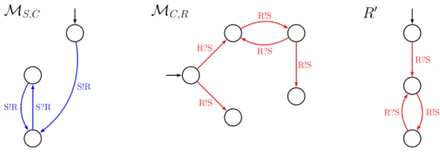
LTSs. The right LTS in Figure 3 is the parallel composition of the middle LTS in the same figure and the right LTS in Figure 1.
Definition 3. An equivalence relation between LTSs is called a congruence for LTSs, denoted by ≡, if for any LTSs L1, L2, L such that L1≡ L2 and any set of
labels Σ one has L1||L ≡ L2||L and L1\ Σ ≡ L2\ Σ.
MLTS. A marked labelled transition system (MLTS), or LTS with marked states, is a tuple ML = (L, F) where L = (Σ, S, T, s0) is an LTS and F ⊆ S is
a set of marked states. According to the set of marked states one can define the set of marked traces MTML of ML as the set of traces for which there exists
a realization verifying some condition on the marked states (examples are given below: automata and B¨uchi automata).
Definition 4. Given MLTSs ML1, ML2 where MLi= (Li, Fi), their parallel
composition ML1||ML2 is the MLTS ML = (L, F) such that L = L1||L2 and
F = F1× F2.
FSA. A finite state automaton (FSA) is an MLTS A = (L, F) such that a trace tr of A is a marked trace if and only if it is finite and it has a realization π = s0t1s1. . . sk such that sk ∈ F. The set MTA is usually called the language
of A.
NBA. A B¨uchi automaton (NBA) is an MLTS B = (L, F) such that a trace tr of B is a marked trace if and only if it is infinite and it has a realization π = s0t1s1t2. . . such that there exists an infinite number of i ≥ 0 for which
si∈ F. As for FSAs, the set MTB is usually called the language of B.
2
Message-passing algorithms
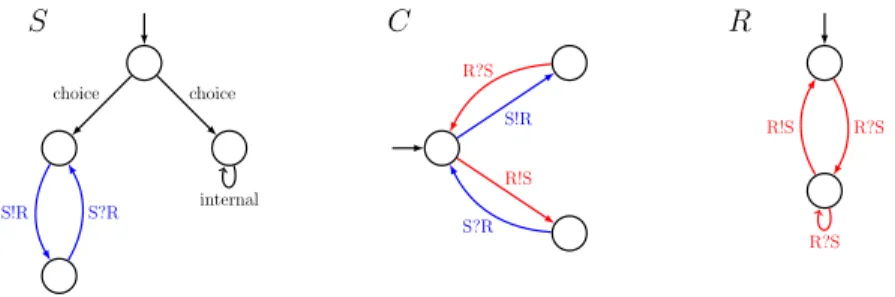
Before presenting a formal description of message-passing algorithms, we illus-trate them on an example. Consider the three LTSs of Figure 1. They represent an abstract view of a small distributed system involving three processes: a sender (S), a capacity one channel (C), and a receiver (R). S has to accomplish some task. It initially does a choice between doing it alone (right transition) or doing it together with R (left transition) by exchanging some messages through C.
The behaviour of this system is captured by L = S||C||R, and so – denoting by ΣS (resp. ΣC, ΣR) the set of labels of S (resp. C, R) – the behaviour of S (resp.
C, R) inside this system is captured by L \ ΣS (resp. L \ ΣC, L \ ΣR).
S choice S!R S?R choice internal C S!R R!S R?S S?R R R?S R!S R?S
Fig. 1. A distributed system constituted of three interacting LTSs.
Definition 5. The interaction graph of a system L1|| · · · ||Ln, where Σi is the
alphabet of Li, has L1, . . . , Ln as nodes, and an edge {Li, Lj} when Σi∩ Σj6= ∅.
The MPAs can solve the reduction problems for systems whose interaction graph is a tree. They proceed by sending messages (which have the same type as the components, i.e. LTSs in our example) along the edges of the tree, i.e. each component sends a message to each of its neighbours. In the system of Figure 1, the interaction graph is a line (and so a tree) with C in the middle and S and R at the extremities (see Figure 2). Indeed S interacts (that is, shares labels) only with C and R also interacts only with C. So each of S and R will send a message to C and C will send a message to each of S and R.
S C R
{S!R, S?R} {R!S, R?S}
MS,C MC,R
Fig. 2. The interaction graph of the system of Figure 1. Over each edge (plain line) the corresponding set of shared labels is indicated. Dashed lines represent the messages propagated from S to R.
The idea behind these messages is the following. In a tree shaped interaction graph, each edge separates the graph into two subtrees whose roots are the extremities of the edge (in our example, the edge (C, R) separates the graph into a tree containing only R and a tree with C as root and S as leaf). Using this fact each component at the extremity of the removed edge will send a message to the other component. This message describes the possible behaviours of the subtree from which its sender is the root as they can be seen by its receiver (for
example C sends a message to R describing the behaviour of S||C as R sees it, that is using only labels shared between C and R). This message is computed from the messages received from the neighbours of its sender in the subtree from which this sender is the root.
In the system of Figure 1 the message from S to C is then MS,C ≡ S \
ΣS∩ ΣC (see Figure 3, left for an example preserving observable traces) and it
is then used to build the message from C to R: MC,R ≡ (MS,C||C) \ ΣC∩ ΣR
(see Figure 3, middle). Similarly the remaining messages can be built: MR,C ≡
R \ ΣR∩ ΣC and MC,S ≡ (MR,C||C) \ ΣC∩ ΣS. It can then be proved (it is
a consequence of Theorem 1 below) using the separation property of the edges of a tree shaped interaction graph described above, that the composition of each component with all the messages it received describes the behaviour of this component in the full system. For example (see Figure 3, right) R0 = R||M
C,R
has the same set of observable traces than L \ ΣR. Similarly S0= S||MC,S and
C0 = C||MR,C||MS,C have the same set of observable traces than L \ ΣS and
L \ ΣC respectively. MS,C S!R S!R S?R MC,R R?S R!S R!S R?S R!S R0 R?S R?S R!S
Fig. 3. Messages from S to R, updated component R0.
2.1 Formal description of an MPA for LTSs
Algorithm 1 below presents a formal description of an MPA for a system L = L1|| . . . ||Ln whose interaction graph G = (V, E) is a tree. Any LTS Ki obtained
at the end of Algorithm 1 is called the update of Li (in G).
For the presentation it is convenient to model an undirected edge {Li, Lj}
as two directed edges (Li, Lj) and (Lj, Li). So the input to Algorithm 1 is a
directed graph G derived from a tree in this way.
We denote by x :≡ L that the variable x is assigned some LTS L0 such that L0 ≡ L. Notice that this is a nondeterministic assignment, and so Algo-rithm 1 is nondeterministic. In the next section we present several instances of the algorithm, and for each one we explain how the nondeterminism is resolved. In order to formulate and prove the correctness of the algorithm we introduce some notations.
Algorithm 1 An MPA for LTSs
Input: an interaction graph G = (V, E) with V = {L1, . . . , Ln}
1: M ← E
2: while M 6= ∅ do
3: choose (Li, Lj) ∈ M such that (Lk, Li) /∈ M for every k 6= j
4: Mi,j:≡ (Li|| (||k 6= j, (Lk, Li) ∈ E Mk,i)) \ Σj 5: remove (Li, Lj) from M 6: end while 7: for all i ∈ V do 8: Ki:≡ Li|| (||(Lj,Li)∈EMj,i) 9: end for
Definition 6. Given G = (V, E) with V = {L1, . . . , Ln}, we denote the parallel
composition (L1|| · · · ||Ln) by bG.
Given a tree G = (V, E) and (Li, Lj) ∈ E, we denote by Gij the maximal subtree
of G containing Lj but not Li.
Lemma 1. Let G = (V, E) be a tree and (Li, Lj) ∈ E. Let MGj,ibe the content of
variable Mj,iafter termination of Algorithm 1 on input G. Then MGj,i= bGij\Σi.
Proof. The proof is by induction on the depth of Gij. If Gijhas depth 1, then G ij
contains the vertex Lj and no arcs. By line 4 we get MGj,i≡ Li\ Σi = bGij\ Σj
(recall that, since we represent undirected trees as directed graphs, we have (Lj, Li) ∈ E).
Assume now that Gij has depth larger than 1. Let L
j1, . . . , Ljm be the
neigh-bours of Lj in Gij. Then the trees Gjj1, . . . Gjjmare proper subtrees of Gij, and
in particular have smaller depth. By induction hypothesis we have MGij
j1,j ≡ bGjj1\ Σj . . . M
Gij
jm,j ≡ bGjjm\ Σj (1)
By line 4 of the algorithm, and since ≡ is a congruence, we get
MGj,i≡ ( Lj|| (||k 6= i, (Lk, Lj ) ∈ E MGk,j) ) \ Σi (2) ≡ ( Lj|| MGj1,j|| · · · || M G jm,j ) \ Σi (3) ≡ ( Lj|| M Gij j1,j|| · · · || M Gij jm,j ) \ Σi (4) ≡ ( Lj|| ( bGjj1\ Σj) || · · · || ( bGjjm\ Σj) ) \ Σi (5)
where (4) follows from (3) because Lk is a node of Gij for every Mk,j.
Since G is a tree, the sets of labels of bGjj1, . . . , bGjjm are pairwise disjoint, and
so
Lj|| ( bGjj1\ Σj)|| · · · ||( bGjjm\ Σj) ≡ (Lj|| bGjj1|| · · · || bGjjm) \ Σj (6)
Moreover, for the same reason, there are no edges between any of Lj1, . . . , Ljm
(Lj|| bGjj1|| · · · || bGjjm) \ Σj\ Σi≡ (Lj || bGjj1|| · · · || bGjjm) \ Σi (7)
Putting together (4)-(7), we obtain
Mj,i≡ (Lj || bGjj1|| · · · || bGjjm) \ Σi (8)
By definition of bGij, we have
b
Gij≡ Lj|| bGjj1|| · · · || bGjjm (9)
which together with (8) yields MG
j,i≡ bGij\ Σi (10)
as desired.
We can now prove correctness of Algorithm 1.
Theorem 1. Let G = (V, E) with V = {L1, . . . , Ln} be a tree-shaped interaction
graph. The result of running Algorithm 1 on G are LTSs K1, . . . , Kn such that
Ki≡ bG \ Σi for every Li∈ V . Proof. We have Ki ≡ Li|| (||(Lj,Li)∈E M G i,j) (11) ≡ Li|| (||(Lj,Li)∈E ( bGij\ Σi)) (12) ≡ Li|| (||(Lj,Li)∈E Gbij) \ Σi (13) ≡ bG \ Σi (14)
Here, (11) follows from line 8 of the algorithm; (12) follows from Lemma 1; (13) follows from the fact that no two neighbours of Liare connected by an edge,
and so their sets of labels are disjoint. Finally, (14) follows from the definitions of bG and bGij.
If the messages of Algorithm 1 are large in the worst case (in theory they can have the size of the full system) their number is optimal. More precisely, no MPA using fewer messages can be correct, where the only assumption we make about MPAs is that the output Kiis a function of Li and the messages Li
receives from its neighbours.
Theorem 2. For every correct MPA algorithm and every n ≥ 1 there is a graph Gn such that the algorithm requires at least 2n − 2 messages on Gn.
Proof. Assume there is a correct MPA A which always requires less than 2n − 2 messages on graphs with n nodes. Consider the system S1= L1|| · · · ||Ln where
for every 1 ≤ i ≤ n the only maximal trace of Li is aiai+1bi+1bi (its interaction
graph is a line). Since the algorithm needs fewer than 2n − 2 messages, there is an index i such that either Li sends no message to Li−1, or sends no message to
Li+1.
In the first case, consider the system S2which is identical to S1, except that
the only maximal trace of Li is aibi+1ai+1bi. For S1 the only maximal trace
of Kn is anan+1bn+1bn, while for S2 the only maximal trace of Kn is anan+1.
Since, by our assumption on MPAs, Li−1does not receive any message from Li,
it returns the same result Kn in both cases, and so the algorithm is incorrect.
In the second case, consider the system S2 which is identical to S1, except
that the only maximal trace of Li+1 is aibi+1ai+1bi, and proceed analogously
with K1instead of Kn.
Observations The restriction to tree-shaped interaction graphs can be weak-ened in several ways.
Communication graphs. We can replace the interaction graph by a potentially smaller communication graph, thus reducing the number of messages.
Definition 7. Let G be any subgraph of an interaction graph. An edge (Li, Lj) ∈
E is redundant if there exists a sequence (Li, Lk1)(Lk1, Lk2) . . . (Lk`, Lj) of edges
such that i 6= km6= j and ΣLkm ⊇ ΣLi∩ ΣLj for every 1 ≤ km6= j.
A communication graph of a system is any subgraph of the interaction graph obtained by iteratively removing redundant edges.
If some communication graph of a system is a tree then all its communication graphs are trees [1]. We then say that the system lives on a tree. The following proposition shows that the MPA can be applied to any system that lives on a tree, even if its interaction graph is not a tree.
Proposition 1. Let G = (V, E) with V = {L1, . . . , Ln} be a tree-shaped
com-munication graph of L = L1|| . . . ||Ln. The result of running Algorithm 1 on G
are LTSs K1, . . . , Kn such that Ki ≡ bG \ Σi for every Li∈ V .
Proof. The proof follows the lines of Theorem 2. We just have to adjust the arguments justifying Equations (6) and (7) in Lemma 1, and Equation (13) in Theorem 2. For (6) and (13) observe that, if the communication graph is a tree, then there are no edges between the neighbours of Lj. Therefore, by the
definition of communication graph, every common label of any two processes in (5) belongs to Σj which suffices to derive (6) and (13).
For (7) we observe that the communication graph also contains no edges between any of Lj1, . . . , Ljm and Li. So we have (Σj1∪ . . . ∪ Σjm) ∩ Li ⊆ Lj,
and so
Tree decompositions. Any system L = L1|| . . . ||Ln can be transformed into an
equivalent one that lives on a tree. This is in itself trivial, since we can always choose this system as one single LTS equivalent to L. However, this destroys the concurrency of the system. In order to preserve as much concurrency as possible we can compute a tree decomposition of a communication graph [18]. Every set {Li1, . . . , Lik} of the decomposition is then replaced by any single LTS
equivalent to the subsystem Li1|| . . . ||Lik. For instance, if the interaction graph
of L1|| . . . ||Ln is a ring with an even number of components, we can take the
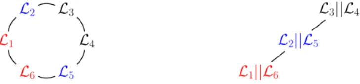
system L01|| . . . ||L0 n/2, where L 0 i≡ Li||Ln−i+1 (Figure 4). L1 L2 L3 L4 L5 L6 L1||L6 L2||L5 L3||L4
Fig. 4. A possible tree decomposition (right) of a ring-shaped interaction graph (left).
Computing one summary. Finally, we observe that computing one single update of component only requires to exchange n − 1 messages instead of 2n − 2. Proposition 2. Let L1, . . . , Ln be LTSs such that the system L = L1|| . . . ||Ln
lives on a tree, and let 1 ≤ i ≤ n. The update Ki of Li can be computed by an
MPA that uses only n − 1 messages.
Proof. Consider a communication graph G = (V, E) of L = L1, . . . , Ln that
is a tree. If n = 1 then i = 1 and L1 = K1 is computed using n − 1 = 0
messages. Assume the proposition is true up to n = k. Consider n = k + 1 and take 1 ≤ i ≤ n. Remark that Ki is computed exactly from the messages
of the form MLj,Li for (Lj, Li) ∈ E (denote by Ei the set containing these
edges). Given such a Lj, consider the largest subtree of G rooted in Lj which
does not contains Li. This subtree has nj < k + 1 nodes, so the update of
Lj in this subtree can be computed from nj− 1 messages. Remark that the
hiding of Σi in this update is exactly MLj,Li. From that Ki is computed using
P
(Lj,Li)∈Ei(nj− 1) + |Ei| = n − 1 messages.
3
Local verification of distributed protocols on trees
In this section we describe our implementations of Algorithm 1, tailored for checking local linear-time safety and liveness properties, respectively. Each im-plementation requires to
– Choose a congruence ≡ that preserves the properties of interest. – Resolve the nondeterminism introduced by :≡ in lines 4 and 8
3.1 Safety
A local safety property of a component Li within a system (L1|| . . . ||Ln) is a
property of the (observable) finite traces of Ki, the update of Li. In order to
preserve local safety properties we choose ≡ as (observable) finite trace equiv-alence, i.e., L ≡ L0 if and only if TL∗ = TL∗0. This equivalence is well known to
be a congruence, and in the following we denote it by ≡T. By Theorem 1, local
safety properties of Li can be decided by examining the traces of its update Ki
returned by Algorithm 1.
We implement L0 :≡T L as follows: L0 is the unique τ -free, minimal
deter-ministic LTS equivalent to L. More precisely,
L0:= M IN (DET (RED(L))),
where RED, DET, M IN are algorithms for removing τ -transitions, determiniz-ing, and minimizing LTSs, respectively. These algorithms are implemented using standard automata operations (see e.g. [19]).
This particular instantiation of Algorithm 1 closely corresponds to the MPA at the basis of the work presented in [2, 3].
3.2 Liveness
It is well known that defining a local liveness property of Lias a property of the
(observable) infinite traces of Ki is inadequate [20]. Consider two systems with
sets of infinite traces {abω} and {abω, acω}, respectively. If Σ
i= {a, b}, then in
both cases the only infinite trace of Ki is abω. However, in the first system Li
satisfies “after a eventually b”, while in the second it does not. To solve this problem we keep information about the divergences of Li.
Definition 8. Given L = (Σ, S, T, s0) with transitions labelled by τ , a diver-gence of L is a finite observable trace tr of L such that there exists an infinite trace tr0 of L verifying tr0|
Σ = tr. The set of divergences of L is denoted by DL.
Given (L1|| . . . ||Ln) without τ -transitions, a divergence of Liin L is a finite
observable trace tri ∈ TL∗i such that there exists an infinite observable trace
tr ∈ Tω
L satisfying tr|Σi = tri.
The hiding operation links these two definitions: Given L = L1|| . . . ||Lnwithout
τ -transitions, the set of divergences of Li in L is equal to the set DL\Σi of
divergences of L \ Σi.
We define a local liveness property of Lias a property of TKiand DL\Σi, and
so we choose: L ≡ L0 if and only if T
L = TL0 and DL = DL0. This equivalence is
known to be a congruence for LTSs (see [21] for example). In the following we denote it by ≡D.
By Theorem 1, local liveness properties of Li can be decided by examining
In order to implement L0:≡D L, we profit from the following fact: for finite
LTSs, TL = TL0 iff T∗
L = TL∗0, and so L ≡D L iff TL∗= TL∗ and DL = DL0. This
allows us to replace the nondeterministic assignment by a five-step procedure: L0:= HID(M IN (DET (RED(DIV (L))))),
where M IN , DET , and RED are defined as above. For L = (Σ, S, T, s0),
DIV (L) is the LTS (Σd, Sd, Td, sd0) such that: Σd = Σ ∪ {τ0} with τ0 ∈ Σ,/
Sd = S, Td = T ∪ Tτ 0 d with T τ0 d = {(s, s) : ∃s 0, s τ L s0 τ L s0}, and s0d = s 0.
Finally, HID(L) is defined as L \ {τ0}, where τ0 has to be the same as used in
DIV . We have:
Theorem 3. L ≡D HID(M IN (DET (RED(DIV (L))))) for any LTS L.
Proof. Denote by Σ the set of labels of L. First remark that a finite sequence tr of labels from Σ is a divergence of L if and only if trτ0ω is an infinite observable trace of DIV (L). This is because (1) tr is a divergence of L if and only if there exists a path realizing tr in L and reaching a state from which there exists an infinite path using only τ -transitions, and (2) DIV (L) is an exact copy of L with the addition of τ0-transitions, all of the form (s, s) for s ∈ S
d = S, and
there is a τ0-transition from a state s to itself if and only if there exists in L an
infinite path using only τ -transitions and starting from s.
From this, and because M IN , DET , and RED preserve observable traces, one gets that a finite sequence tr of labels from Σ is a divergence of L if and only if trτ0ωis an infinite observable trace of M IN (DET (RED(DIV (L)))). Also remark that M IN (DET (RED(DIV (L)))) does not contain any τ -transition.
The remark that HID only replaces τ0-transitions by τ -transitions then al-lows to conclude that a finite sequence tr of labels from Σ is a divergence of L if and only if trτωis an infinite trace of HID(M IN (DET (RED(DIV (L))))) if
and only if tr is a divergence of HID(M IN (DET (RED(DIV (L))))).
4
Experimental evaluation
The approaches described in the previous section have been implemented as an extension of the planner Distoplan [3]. In this section we report on an experi-mental evaluation of the performances of this implementation on two protocols: a mutual exclusion algorithm on trees [4] and the pragmatic general multicast protocol [5]. All experiments were performed using the same computer with an Intel Core i5 processor and a memory limit set to 4GB.
4.1 Raymond’s mutual exclusion protocol.
In [4], Raymond presents a distributed protocol ensuring mutual exclusion for n processes organized as a tree. Processes communicate by rendez-vous, which allows us to model the protocol as a parallel composition of LTSs, one for each process. The unique communication graph is given by the tree. The scaling
parameter is the number of processes, which fits well with our approach as the difference between two instances of the protocol is due to the number of LTSs needed to model them, rather than to their sizes.
The protocol can be roughly described as follows. A single token is passed between the processes, a process being allowed to access its critical section only if it owns the token. At any time, each process Pi not holding the token knows
which of its neighbours in the tree is closest to the token. In other words Piknows
in which maximal subtree containing exactly one of its neighbours, but not Pi
itself, the token currently is. Its requests for the token (and all requests by other processes that it may have to transmit) are sent to this particular neighbour. A more precise description of this protocol is given in Algorithm 2. It describes in a Promela-like manner an agent called x. N denotes the set of neighbours of x in the tree of agents on which the protocol is executed. We consider that x ∈ N . Q(N ) denotes the set of queues of elements from N . Notice that the same element never appears twice in the queue requestQ. At each step one of three mutually exclusive guarded atomic instruction sequences is executed: (1) re-assignation of the token when x holds it, (2) request for the token, (3) non-deterministic choice between: asking for entering the critical section, receiving a request message from a neighbour, receiving the token from a neighbour, deciding to exit the critical section.
Algorithm 2 An agent for Raymond’s mutual exclusion protocol
Agent x (holder: N , using: {true, f alse}, requestQ: Q(N ), asked: {true, f alse}) holder=x ∧ using=f alse
∧ isnotempty(requestQ) → holder:=dequeue(requestQ) asked:=f alse
holder=x → using:=true holder6=x → !token to holder holder6=x ∧ asked=f alse
∧ isnotempty(requestQ) → !request(x) to holder asked:=true else → isnotin(x,requestQ) → enqueue(x,requestQ)
?request(n) → enqueue(n,requestQ) ?token → holder:=x
using=true → using:=f alse
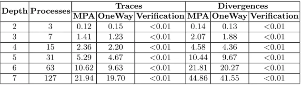
We consider instances of this protocol in which processes form a complete binary tree. The results obtained are presented in Table 1. The leftmost columns give the depth of the binary tree considered (Depth) and the corresponding number of processes (Processes). For each depth the column Traces reports the time (in seconds) needed for the following tasks: (1) run Algorithm 1 to obtain the updated versions of all the processes with respect to trace equivalence ≡T
(subcolumn MPA); (2) same but computing only n − 1 messages in order to obtain the updated version of the root only (subcolumn OneWay); (3) verify a simple local property from the updated root (subcolumn Verification). Column
Divergences gives the times required by analogous tasks, but with respect to divergence equivalence ≡D.
Table 1. Results for the analysis of Raymond’s mutual exclusion protocol on complete binary trees. Times are in seconds.
Depth Processes Traces Divergences
MPA OneWay Verification MPA OneWay Verification
2 3 0.12 0.15 <0.01 0.14 0.13 <0.01 3 7 1.41 1.23 <0.01 2.07 1.88 <0.01 4 15 2.36 2.20 <0.01 4.58 4.36 <0.01 5 31 5.29 4.67 <0.01 10.44 9.67 <0.01 6 63 10.62 9.63 <0.01 21.81 20.27 <0.01 7 127 21.94 19.70 <0.01 44.86 41.55 <0.01
We check a safety (in the case of ≡T) and a liveness (in the case of ≡D)
property in order to compare our MPA with an algorithm that constructs the state space, for which we use Spin. The local safety property verified for the root processes is: “It is not possible to request the token twice without receiving it in between”. Remark that, it is also expressible as the following global property: “It is not possible for the root process to request the token twice without receiving it in between”. We verify this property by checking emptiness of the product of the automaton ϕ on the left of Figure 5 (representing the negation of the property) and the (projection onto the labels of ϕ of the) updated version of the root process obtained by Algorithm 1 (in which all states are considered accepting). The local liveness property verified for the root processes is: “The token is received in finite time after any request”. Similarly, the property is verified by checking emptiness of the product of the B¨uchi automaton ϕ0 on the right of Figure 5 (representing the negation of the property) with the (projection on the labels of ϕ0 of the) updated version of the root process obtained by Algorithm 1 (in which all states are considered accepting).
ϕ
!request ?token !request !requestϕ
0 !request τ τ !request ?tokenFig. 5. Two properties to be checked on Raymond’s mutual exclusion protocol. !request is a general token request action and ?token is a general token reception action.
Analysis of the results. As expected, the approach scales very well with the number of components: at each depth the number of components almost doubles while the time spent for computing the updates of the components is slightly
more than doubling. We compare it with a verification of the same properties using Spin [22]. Since the system is highly concurrent, we use Spin with the partial order reduction optimization. Spin outperforms our approach for the complete binary tree of depth 2 (it needs less than 0.01 seconds to verify the properties). For trees of depth 3 or greater, however, Spin runs out of memory (memory limit being 4GB). Notice that, since the properties we check are true, Spin needs a full state-space exploration to verify them, while our MPA prevents this. We also remark that the time needed by our MPA is almost entirely spent in computing the updates of the components, and so the additional cost of veri-fying other properties after the first one is small, since the previously computed updates can be re-used. Finally, observe that, in this example, the difference in time spent between the standard application of Algorithm 1 (computing all updates) and the case where only the update of the root is computed (so only half of the messages are constructed) is not significant. This can be explained by the fact that – being the initial owner of the token – the root imposes more constraints to the system than the other components. So the messages from the root are potentially much simpler to compute than the messages to the root.
4.2 The pragmatic general multicast protocol.
[5] describes the pragmatic general multicast protocol (PGM), a reliable dis-tributed protocol for distributing information from multiple senders to multiple receivers in a network, designed to minimize the load of the network due to acknowledgement messages and retransmissions of lost messages. We consider the specific version of this very generic protocol given in Algorithm 3 (which is almost the one described in [17]): a unique source sends information to multi-ple receivers in a network organized as a tree. Each process is described in a Promela-like manner and consists of a single loop in which a non-deterministic choice is done at each step between several guarded atomic instruction sequences. The source can receive a negative acknowledgement nak(nr) for some data, in this case it sends back a confirmation ncf (nr) and, if the data nr is still within range of its window it adds it to the set recN ak of data to be re-sent. If some data nr is in the set recN ak and still within range of the window this data can be re-sent as a message rdata(nr, txW T r). And, if no data needs to be re-sent, a new data can be sent as a message odata(nr, txW T r) and the window may be moved. Any network element can receive negative acknowledgements and propagate them above itself in the tree. It can also transmit data below itself in the tree. Finally, it may generate new negative acknowledgements while no confirmation have been received for them. A receiver can receive data, and, when it allows it to deduce that some data are missing (by looking at the previously received data and because of the fact that the data are consecutive integers) it can send negative acknowledgements for these data.
As before we represent each process by an LTS. However, communications are no longer by rendez-vous but use messages sent through bidirectional channels (which can lose messages). Each channel is thus also modelled as an LTS. The unique communication graph of such a system is a tree.
Algorithm 3 PGM: source, network elements, and receivers
Source (data: N, winSize: N, txWTr: N, recNak: 2N)
?nak(nr) → !ncf(nr) txWTr < nr → recNak := add(recNak,nr) isin(nr,recNak) → nr > txWTr → !rdata(nr,txWTr) recNak := remove(recNak,nr) lenght(recNak) = 0 → !odata(data,txWTr) data := data + 1
odata > winSize + txWTr → txWTr := txWTr + winSize Network element (setRepair: 2N)
?nak(nr) → setRepair := add(setRepair,nr)
isnotin(setRepair,nr) → !nak(nr) upwards !ncf(nr) downwards
?rdata(nr,txWTr) → setRepair := remove(setRepair,nr) !rdata(nr,txWTr) downwards ?ncf(nr) → setRepair := remove(setRepair,nr) ?odata(nr,txWTr) → !odata(nr,txWTr) downwards isin(nr,setRepair) → !nak(nr) upwards
Receiver (rxWTr: N, setNr: 2N, setMissing: 2N)
?odata(nr,txWTr) ∧ rxWTr < nr → rxWTr < txWTr → rxWTr := txWTr setNr := add(setNr,nr)
for all (rxWTr < i < nr ∧ isnotin(i,setNr)) setMissing := add(setMissing,i) setMissing := remove(setMissing,nr) ?rdata(nr,txWTr) ∧ rxWTr < nr → rxWTr < txWTr → rxWTr := txWTr setNr := add(setNr,nr) setMissing := remove(setMissing,nr) isin(nr,setMissing) → nr > rxWTr → !nak(nr) nr ≤ rxWTr setMissing := remove(setMissing,nr)
In our experiments we considered two possible topologies for the systems: lines and complete binary trees. In each of these cases we considered instances of the protocol with increasing numbers of processes. We also made other pa-rameters vary: the number of different data to be sent by the source (two or three) and the capacity of the channels (one or two messages). The initial value of data for the source is set to 1 and the value of winSize is set to anything higher than the number of different data to be sent. All other integer parameters are initialized to 0 and all sets are initially empty.
Figure 6 presents the update of a leaf as obtained by Algorithm 1 (using ≡T as congruence) when ran on a complete binary tree of depth five with two
data to be sent and channels of capacity one. It is interesting to notice that just by looking at this LTS, a behaviour (corresponding to the path with larger labels in the figure) that may not be directly anticipated from the description of the protocol can be remarked: it is possible for the leaf to deduce that the
second (and last) data will never be received. This can in fact be explained by the possible losses of messages. For sure ncf (1) has been sent (by the source after reception of nak(1) from another leaf) after odata(2, 0). So, each channel between the source and the leaf represented in Figure 6 has contained ncf (1) at some time, and if it has contained odata(2, 0) at some time it was before ncf (1). The only explanation for receiving ncf (1) before odata(2, 0) is thus a loss of odata(2, 0) at some channel.
?ncf(1) ! n a k ( 1 ) ?ncf(1) ! n a k ( 1 ) ? r d a t a ( 1 , 0 ) ! n a k ( 1 ) ? r d a t a ( 1 , 0 ) ?ncf(1) ? r d a t a ( 1 , 0 ) ! n a k ( 1 ) ?ncf(1) ? r d a t a ( 1 , 0 ) ? r d a t a ( 1 , 0 ) ? o d a t a ( 2 , 0 ) ? n c f ( 1 ) ? o d a t a ( 2 , 0 ) ? o d a t a ( 1 , 0 )
Fig. 6. PGM protocol: update of a leaf in a complete binary tree of depth five when the number of different data to be sent is two and the channels capacity is one.
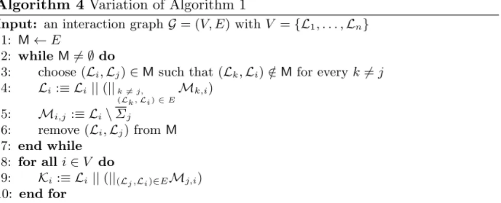
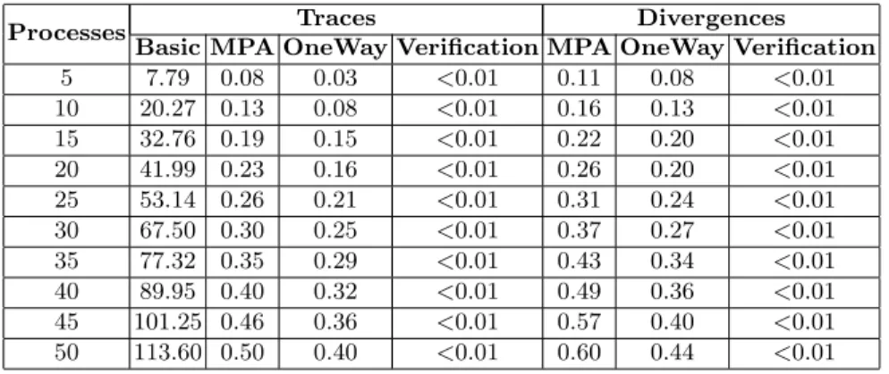
Table 2 gives the results obtained for the PGM protocols on lines, in the case where the source can only send two different data and the channels are of capacity one. Results are organized as before. The only difference are in the Basic and MPA columns. The Basic column presents the times obtained by run-ning Algorithm 1 while the MPA columns present the times obtained by runrun-ning Algorithm 4. This algorithm is a variation of Algorithm 1 where messages that “cross” at some edge of the communication graph are not completely indepen-dent: the constraints imposed by the first to be computed are used to compute the second.
Algorithm 4 Variation of Algorithm 1
Input: an interaction graph G = (V, E) with V = {L1, . . . , Ln}
1: M ← E
2: while M 6= ∅ do
3: choose (Li, Lj) ∈ M such that (Lk, Li) /∈ M for every k 6= j
4: Li:≡ Li|| (||k 6= j, (Lk, Li) ∈ E Mk,i) 5: Mi,j:≡ Li\ Σj 6: remove (Li, Lj) from M 7: end while 8: for all i ∈ V do 9: Ki:≡ Li|| (||(Lj,Li)∈EMj,i) 10: end for
The local safety and liveness properties we check at the source are the fol-lowing: “The last data can only be sent once” (its negation is represented by
the FSA ϕ on the left of Figure 7) and “The first data is always sent at least once” (its negation is represented by the NBA ϕ0 on the right of Figure 7). The verification process is the same as above.
ϕ
!maxdata !maxdataϕ
0 !mindataτ
Fig. 7. Two properties to be checked on PGM. !maxdata (respectively !mindata) rep-resents any sending of the last data (respectively the first data) using an odata or an rdata message.
Table 3 gives the other results obtained for the PGM protocols on lines. Table 4 gives the results obtained for the PGM protocols on complete binary trees. They only report the running times of Algorithm 4 as the verification of the properties considered still always requires less than 0.01 seconds.
Analysis of the results. Spin can deal with lines of length 5 within 20 seconds but cannot handle larger lines nor binary trees without running out of the 4GB of memory allowed to it. In addition to what has been noticed in the case of Raymond’s mutual exclusion protocol, it appears that using Algorithm 4 instead of Algorithm 1 can significantly reduce running times. This is due to the fact that some constraints are taken into account earlier, and so some messages can be simplified. Using this version of our approach is not always that efficient however. In the case of Raymond’s mutual exclusion protocol, for example, it almost does not reduce running times. The comparison of the different numbers of data and capacities of channels also shows that, if our approach scales well with the number of components of the system to analyse, it is more sensitive to increases of the sizes of these components.
Conclusion
We have presented message-passing algorithms for the verification of local prop-erties of distributed protocols. The components of the protocol must have a tree-shaped communication structure. The MPAs compute for each component Li an LTS equivalent to the result of hiding in the full LTS (the LTS of the full
protocol) all actions not appearing in Li. We have shown that the MPAs can be
instantiated with different equivalence notions, in particular trace equivalence and divergence equivalence. We have evaluated the algorithms on two well-known protocols, and shown that for several important properties they scale very well, in particular much better than a generic search-based model-checker like Spin.
The properties we have used for our comparison with Spin were true proper-ties, i.e., properties that hold for the protocol. In fact, for false properties Spin often outperforms our approach, possibly due to the existence of a relatively
Table 2. Analysis of PGM (with two different data and channels of capacity one) on lines. Times are in seconds.
Processes Traces Divergences
Basic MPA OneWay Verification MPA OneWay Verification
5 7.79 0.08 0.03 <0.01 0.11 0.08 <0.01 10 20.27 0.13 0.08 <0.01 0.16 0.13 <0.01 15 32.76 0.19 0.15 <0.01 0.22 0.20 <0.01 20 41.99 0.23 0.16 <0.01 0.26 0.20 <0.01 25 53.14 0.26 0.21 <0.01 0.31 0.24 <0.01 30 67.50 0.30 0.25 <0.01 0.37 0.27 <0.01 35 77.32 0.35 0.29 <0.01 0.43 0.34 <0.01 40 89.95 0.40 0.32 <0.01 0.49 0.36 <0.01 45 101.25 0.46 0.36 <0.01 0.57 0.40 <0.01 50 113.60 0.50 0.40 <0.01 0.60 0.44 <0.01
Table 3. Analysis of PGM on lines using Algorithm 4. Different numbers of data to be sent (d) and different sizes of channels (c) are considered. Times are in seconds.
Processes Traces Divergences
d=2, c=2 d=3, c=1 d=2, c=2 d=3, c=1 5 10.71 10.63 15.37 13.26 10 19.19 12.60 28.94 18.00 15 27.24 14.56 41.77 22.21 20 35.53 16.46 55.77 26.80 25 43.66 18.24 68.40 30.95 30 52.14 20.66 81.43 35.36 35 60.16 22.64 95.39 39.82 40 68.78 24.80 109.17 44.49 45 77.00 26.66 122.57 48.56 50 85.12 29.01 136.60 53.27
Table 4. Analysis of PGM on complete binary trees using Algorithm 4. Different numbers of data to be sent (d) and different sizes of channels (c) are considered. Times are in seconds.
Depth Proc. Traces Divergences
d=2, c=1 d=2, c=2 d=3, c=1 d=2, c=1 d=2, c=2 d=3, c=1 3 7 0.85 26.26 59.30 1.41 33.96 93.02 4 15 1.58 56.10 114.05 1.60 72.89 156.93 5 31 2.48 113.82 235.32 2.93 153.47 316.63 6 63 5.06 231.27 472.19 5.73 310.28 641.13 7 127 10.24 474.57 979.85 12.10 625.61 1582.23
large number of counterexamples, which allows Spin to quickly find one. This suggests to run Spin and a suitable MPA in parallel.
Future work will explore how to instantiate the MPAs with equivalence re-lations sensitive to deadlocks or partial deadlocks.
References
1. E. Fabre. Bayesian Networks of Dynamic Systems. Habilitation `a diriger des recherches, Universit´e de Rennes1, 2007.
2. E. Fabre and L. Jezequel. Distributed optimal planning: an approach by weighted automata calculus. In CDC, pages 211–216, 2009.
3. E. Fabre, L. Jezequel, P. Haslum, and S. Thi´ebaux. Cost-optimal factored planning: Promises and pitfalls. In ICAPS, pages 65–72, 2010.
4. K. Raymond. A tree-based algorithm for distributed mutual exclusion. TCS, 7(1):61–77, 1989.
5. T. Speakman et al. PGM reliable transport protocol specification. RFC 3208 (Experimental) of the IETF, 2001.
6. J. M. Cobleigh, D. Giannakopoulou, and C. S. Pasareanu. Learning assumptions for compositional verification. In TACAS, pages 331–346, 2003.
7. C. Flanagan and S. Qadeer. Thread-modular model checking. In SPIN, pages 213–224, 2003.
8. S. Graf and B. Steffen. Compositional minimization of finite state systems. In CAV, pages 186–196, 1990.
9. O. Grumberg and D. E. Long. Model checking and modular verification. TOPLAS, 16(3):843–871, 1994.
10. A. W. Roscoe, P. H. B. Gardiner, M. H. Goldsmith, J. R. Hullance, D. M. Jackson, and J. B. Scattergood. Hierarchical compression for model-checking CSP or how to check 1020 dining philosophers for deadlock. In TACAS, pages 133–152, 1995.
11. FRD2 user manual, 2009.
12. R. Cleaveland, J. Parrow, and B. Steffen. The concurrency workbench: A semantics-based tool for the verification of concurrent systems. TOPLAS, 15(1):36– 72, 1993.
13. H. Garavel, F. Lang, R. Mateescu, and W. Serwe. CADP 2011: a toolbox for the construction and analysis of distributed processes. STTT, 15(2):89–107, 2013. 14. P. A. Abdulla. Regular model checking. STTT, 14(2):109–118, 2012.
15. B. B´erard, P. Bouyer, and A. Petit. Analysing the PGM protocol with UPPAAL. International journal of production research, 42(14):2773–2791, 2004.
16. M. Boyer and M. Sighireanu. Synthesis and verification of constraints in the PGM protocol. In FME, pages 264–281. Springer, 2003.
17. J. Esparza and M. Maidl. Simple representative instantiations for multicast pro-tocols. In TACAS, pages 128–143, 2003.
18. H. Bodlaender. A linear time algorithm for finding tree-decompositions of small treewidth. In STC, pages 226–234, 1993.
19. J. Sakarovitch. ´El´ements de th´eorie des automates. Vuibert, 2003.
20. S. D. Brookes and A. W. Roscoe. An improved failures model for communicating processes. In Seminar on Concurrency, pages 281–305, 1984.
21. A. Valmari. All linear-time congruences for finite LTSs and familiar operators. In ACSD, 2012.
22. G. Holzmann. The SPIN model checker: primer and reference manual. Addison-Wesley Professional, 2003.