TopPI: An efficient algorithm for item-centric mining

HAL Id: hal-01479067

https://hal.archives-ouvertes.fr/hal-01479067

Submitted on 28 Feb 2017

HAL is a multi-disciplinary open access

archive for the deposit and dissemination of

sci-entific research documents, whether they are

pub-lished or not. The documents may come from

L’archive ouverte pluridisciplinaire HAL, est

destinée au dépôt et à la diffusion de documents

scientifiques de niveau recherche, publiés ou non,

émanant des établissements d’enseignement et de

TopPI: An efficient algorithm for item-centric mining

Vincent Leroy, Martin Kirchgessner, Alexandre Termier, Sihem Amer-Yahia

To cite this version:

Vincent Leroy, Martin Kirchgessner, Alexandre Termier, Sihem Amer-Yahia.

TopPI: An

effi-cient algorithm for item-centric mining.

Information Systems, Elsevier, 2017, 64, pp.104 - 118.

�10.1016/j.is.2016.09.001�. �hal-01479067�

TopPI: An Efficient Algorithm for Item-Centric Mining

V. Leroya,∗, M. Kirchgessnera, A. Termierb, S. Amer-Yahiaa

a_{Univ. Grenoble Alpes, LIG, CNRS, F-38000 Grenoble, France} b_{Univ. Rennes 1, IRISA, INRIA, F-35000 Rennes, France}

Abstract

In this paper, we introduce item-centric mining, a new semantics for mining long-tailed datasets. Our algorithm, TopPI, finds for each item its top-k most frequent closed itemsets. While most mining algorithms focus on the globally most frequent itemsets, TopPI guarantees that each item is represented in the results, regardless of its frequency in the database.

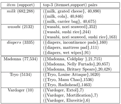
TopPI allows users to efficiently explore Web data, answering questions such as “what are the k most common sets of songs downloaded together with the ones of my favorite artist?”. When processing retail data consisting of 55 million supermarket receipts, TopPI finds the itemset “milk, puff pastry” that appears 10,315 times, but also “frangipane, puff pastry” and “nori seaweed, wasabi, sushi rice” that occur only 1120 and 163 times, respectively. Our experiments with analysts from the marketing department of our retail partner, demonstrate that item-centric mining discover valuable itemsets. We also show that TopPI can serve as a building-block to approximate complex itemset ranking measures such as the p-value.

Thanks to efficient enumeration and pruning strategies, TopPI avoids the search space explosion induced by mining low support itemsets. We show how TopPI can be parallelized on multi-cores and distributed on Hadoop clusters. Our experiments on datasets with different characteristics show the superior-ity of TopPI when compared to standard top-k solutions, and to Parallel FP-Growth, its closest competitor.

Keywords: Frequent itemset mining, Top-K, Parallel data mining, MapReduce

2000 MSC: 68W15

1. Introduction

Over the past twenty years, pattern mining algorithms have been applied successfully on various datasets to extract frequent itemsets and uncover hidden

∗_{Corresponding author}

Email addresses: vincent.leroy@imag.fr (V. Leroy), martin.kirchgessner@imag.fr (M. Kirchgessner), Alexandre.Termier@imag.fr (A. Termier), Sihem.Amer-Yahia@imag.fr (S. Amer-Yahia)

Support C

ount

Items

Support threshold

(a) Frequent Itemset Mining

Support C

ount

Items

k

(b) Our approach, TopPI

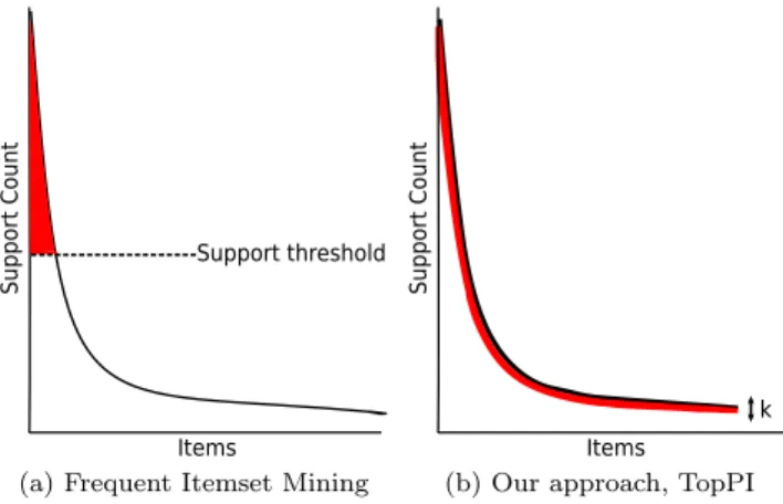
Figure 1: Schematic distinction between frequent itemsets mining and TopPI. The area in red represent each method’s output.

associations [1, 2]. As more data is made available, large-scale datasets have proven challenging for traditional itemset mining approaches. Since the worst-case complexity of frequent itemset mining is exponential in the number of items in the dataset, analysts have been using high support threshold thus estricting the mining to the globally most frequent itemsets. However, many large datasets today exhibit a long tail distribution, characterized by the presence of a majority of infrequent items [3]. Mining at high thresholds eliminates low-frequency items, thus ignoring most of the data (Figure 1a). In this paper, we propose item-centric mining, a new semantics that is more appropriate to mining long-tailed datasets. We design TopPI, an efficient algorithm that implements this new semantics, and develop centralized and distributed versions of TopPI.

Frequent itemsets mining (FIM) was popularized by the famous “beer and diapers” association [1]. A common request in the retail industry is the ability to access a product’s sales trends and associations with other products. This allows managers to obtain feedback on customer behavior and to propose relevant product bundles. Traditional FIM algorithms, however, fail to find itemsets for a majority of products. Their results are often dominated by the most frequent products (typically occurring less than 5% of the time). On long-tailed datasets, where the majority of items appear a few times, traditional FIM misses most of the data as illustrated in Figure 1a. We hence formalize our objective as follows: extract, for each item, the k most frequent itemsets containing that item. This new semantics, coined item-centric mining, guarantees to return itemsets for each item including those with very low frequency.

We present experiments on two real datasets: 55 million supermarket re-ceipts (over 389,372 products) and the favorite artists of 1.2 million users of LastFM (see Section 5.1 for more details). Table 1 contains example itemsets that we generated from these datasets, along with their frequencies. The ex-amples contain itemsets whose support range from 10 to 682,288. Item-centric

item (support) top-3 (itemset,support) pairs milk (682,288) ({milk, grated cheese}, 40,890)

({milk, cola}, 40,846) ({milk, carrier bag}, 40,675) wasabi (2132) ({wasabi, nori seaweed},352)

({wasabi, sushi rice},244)

({wasabi, nori seaweed, sushi rice},163) diapers (3335) ({diapers, incontinence pads},160)

({diapers, mattress pad},111) ({diapers, wet wipes},91) Madonna (77,534) ({Madonna, Coldplay },21,715)

({Madonna, Nelly Furtado},20,857) ({Madonna, Britney Spears},20,428) Tryo (5134) ({Tryo, Louise Attaque},1620)

({Tryo, Manu Chao},1536) ({Tryo, Radiohead},1463) Vardoger (10) ({Vardoger, Extol},7)

({Vardoger, Mortification},7) ({Vardoger, Eluveitie},6)

Table 1: TopPI results for k = 3 on retail and music datasets. “Tryo” is associated to two other french alternative-rock bands, and “Vardoger” with similar metal bands.

itemsets provide the analyst with an overview of the dataset more suitable for further exploration (Figure 1b). That is relevant for retail datasets but also for query recommendations [2]. In the latter, recommendation queries can be computed for rare terms.

Item-centric mining raises a new challenge, namely minimizing the itemsets exploration while guaranteeing correctness and completeness. In order to handle large datasets in a reasonable amount of time, the solution must also allow an efficient parallelization.

We design TopPI, an algorithm able to drive the itemsets exploration towards solutions of interest with a negligible overhead. In TopPI, the solution space is shaped as a tree, following LCM [4]. TopPI constructs its results set in memory, and uses that to dynamically prune the search space as it is traversed. By searching k itemsets for all items at once, pruning is shared between different exploration branches.

In a distributed environment, the challenge is to preserve this pruning power without inter-node communications. TopPI addresses this issue by splitting the mining into two phases. In the first one, each worker substantially limits its itemsets exploration, using only local data, and computes a few statistics about its branches’ first results. These statistics are shared between all workers, and used in the second mining phase to find the remaining results only.

FIM algorithms rely on a user-provided frequency threshold to reduce the the input size and limit exploration. TopPI, instead, computes an adequate

threshold for each branch. The analyst only has to set the parameter k, which controls the number of itemsets returned for each item. If the itemsets are directly presented to an analyst, k = 10 can be sufficient, while k = 1000 may be used when itemsets are analyzed automatically.

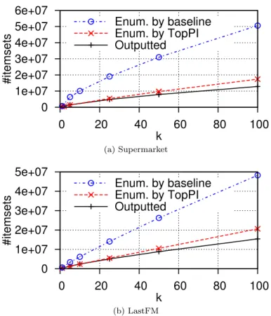
We run experiments on a multi-core machine and a Hadoop cluster. We first compare TopPI to its most obvious competitor that computes a global top-k with a very low support threshold (itemsets that appear at least twice). Our baseline is an implementation of TFP[5] and its parallelization with 32 threads. We show that TopPI significantly outperforms its baseline, which fails to output results in some cases (taking over 8 hours to complete or running out of memory). The problem of finding top-k itemsets for each item is not anti-monotone, thus we have to enumerate a few non-solution itemsets to reach some solutions. But we observe that the baseline enumerates many more intermediate solutions. Thanks to the use of appropriate heuristics to guide the exploration, TopPI only enumerates a small fraction of discarded itemsets. On our music dataset, when k = 100, the output contains approximately 12.8 million distinct itemsets. The baseline enumerates 50.6 million itemsets and TopPI only 17.4 millions.

We then evaluate the centralized parallel version of TopPI and examine the mining time speedup with respect to the number of mining threads. We find that using 16 threads is a sweet spot for high performance. Above that number, the memory bus starts to become a bottleneck. Indeed threads compete for memory accesses when building their reduced datasets, which triggers massive accesses to non-consecutive areas of the memory. We show that TopPI is able to mine our music dataset with k = 50 and a support equal to 2 on a laptop with 4 threads (Intel Core i7-3687U) and 6 GB of RAM in 16 minutes. To attain a similar level of performance, PFP [2], our closest competitor, requires a distributed setting with 200 cores.

TopPI relies on frequency to rank each of the k itemsets associated with an item. The itemsets associated with each item can also be ranked using their statistical correlation with that item, such as the p-value. However, ranking by p-value implies a much wider exploration of the itemsets’ space, which is not affordable at our scale. We hence explore the quality of our results and compare it to ranking itemsets by p-value. We show experimentally that, while being faster, the output of TopPI is very close to tok itemsets ranked by p-value. We also conduct a user study with marketing experts that shows the high quality of extracted itemsets.

The paper is organized as follows. Section 2 contains some preliminaries, defines the item-centric mining semantics and recalls basic principles of itemsets’ mining. The TopPI algorithm is fully described in Section 3. Its MapReduce version is detailed in Section 4. In Section 5, we present experimental results and compare TopPI against TFP [5] and PFP [2], the two closest works. We evaluate the quality of association rules uncovered by TopPI on retail datasets, in Section 6. Related work is reviewed in Section 7, and we conclude in Section 8.

TID Transaction t0 {0, 1, 2} t1 {0, 1, 2} t2 {0, 1} t3 {2, 3} t4 {0, 3} (a) Input D

item top(i): P , support (P )

i 1st ₂nd

0 {0}, 4 {0, 1}, 3 1 {0, 1}, 3 {0, 1, 2}, 2 2 {2}, 3 {0, 1, 2}, 2 3 {3}, 2

(b) TopPI results for k = 2 Table 2: Sample dataset

2. Item-Centric Mining 2.1. Preliminaries

The data contains items drawn from a set I. Each item has an integer identifier, referred to as an index, which provides an order on I. A dataset D is a collection of transactions, denoted {t1, ..., tn}, where tj ⊆ I. An itemset

P is a subset of I. A transaction tj is an occurrence of P if P ⊆ tj. Given

a dataset D, the projected dataset for an itemset P is the dataset D restricted to the occurrences of P : D[P ] = {t | t ∈ D ∧ P ⊆ t}. In the example dataset shown in Table 2a, D[{0, 1}] = {t0, t1, t2}. To further reduce its size, all items

of P can be removed, giving the reduced dataset of P : DP = {t \ P | t ∈ D[P ]}.

Hence, in the example, D{0,1}= {{2}, {2}, {}}.

The number of occurrences of an itemset in D is called its support and denoted support_D(P ). More formally, support_D(P ) = support_{D[P ]}(P ) = |DP|.

An itemset P is said to be closed if there exists no itemset P0 ⊃ P such that support (P ) = support (P0). The greatest itemset P0 ⊇ P having the same support as P is called the closure of P , further denoted as clo(P ). For example, in the dataset shown in Table 2a, the itemset {1, 2} has a support equal to 2 and clo({1, 2}) = {0, 1, 2}.

2.2. The item-centric mining problem

Given a dataset D and an integer k, our goal is to return, for each item in D, the k most frequent closed itemsets containing this item. Table 2b shows the solution to this problem applied to the dataset in Table 2a with k = 2. Note that we purposely ignore itemsets that occur only once, as they do not show a behavioral pattern.

2.3. Key principles of closed frequent itemsets enumeration

Several algorithms aim at mining closed itemsets (CIS) present in a dataset [5– 7]. For efficiency reasons, TopPI borrows some principles developed for the LCM algorithm [4]: the closure extension, that generates new CIS from previously computed ones, and the first parent that avoids redundant computation. We define these principles below.

clo(∅) = ∅1 {0}, 42 {0, 1}, 33 {2}, 34 {0, 1, 2}, 25 {0, 1, 2}, 26 {3}, 27 h∅, 0i h∅, 1i h∅, 2i h∅, 3i h{2}, 0i h{2}, 1i

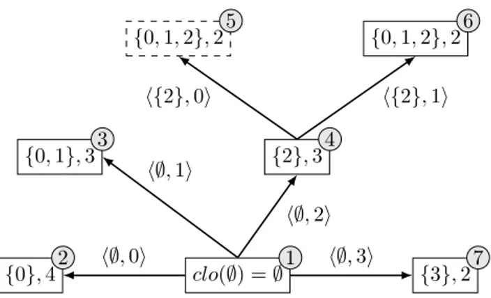
Figure 2: CIS enumeration tree on our example dataset (Table 2a). hP, ii denotes the closure extension operation.

Definition 1. An itemset Q ⊆ I is a closure extension of a closed itemset P ⊆ I if ∃e /∈ P , called an extension item, such that Q = clo(P ∪ {e}).

TopPI enumerates CIS by recursively performing closure extensions, starting from the empty set. In this context, pruning the solution space means avoiding one or many recursive calls. In Table 2a, {0, 1, 2} is a closure extension of both {0, 1} and {2}. This example shows that, starting from simple itemsets of size 1, a new itemset of size 2 can be generated by two different closure extensions. Uno et al. [7] introduced two principles which guarantee that each closed itemset is traversed only once in the exploration. We adapt their principles as follows. First, extensions are restricted to items smaller than the previous extension. Furthermore, we prune extensions that do not satisfy the first-parent criterion: Definition 2. Given a closed itemset P and an item e /∈ P , hP, ei is the first parent of Q = clo(P ∪ {e}) only if max (Q \ P ) = e.

The extension enumeration order and the first parent test shapes the closure extensions lattice as a tree. Figure 2 shows the itemsets tree for the dataset in Table 2a. h{2}, 1i is the first parent of {0, 1, 2}, but h{2}, 0i is not. Therefore the branch produced by h{2}, 0i is pruned.

These enumeration principles also lead to the following property: by ex-tending P with e, TopPI can only recursively generate itemsets Q such that max (Q \ P ) = e. As we detail in Section 4, this is fundamental to parallelize both the CIS enumeration and TopPI’s pruning.

Example enumeration. Figure 2 shows how and in which order CFIS are enu-merated in TopPI on the sample dataset of Table 2a. The itemsets generated by extending a closed itemset P are located in the sub-tree rooted at P .

1 The algorithm starts by checking if any item in D appears in all trans-actions. Such items belong to the empty itemset’s closure, clo(∅). As in most

cases, here clo(∅) is empty. The empty set is therefore used as the initial item-set. It is extended by each frequent item in D, called starter items. 2 The first starter is 0, and {0} is a closed itemset so the algorithm stores it. Given that 0 is the smallest item, no recursion happens. 3 The next starter is 1, which generates by closure the itemset {0, 1}. Given that 1 > 0, the closure satisfies the first parent test and {0, 1} is stored. The only remaining item in D{0,1}is 2,

but it’s greater than the previous extension item, so no recursion happens. 4 The following starter is 2, leading to {2}, a closed singleton. Two frequent items, smaller than 2, remain in D_{2} so the enumerator performs recursive extensions of {2}. 5 The algorithm first extends {2} with 0 which, by closure, generates the pattern {0, 1, 2}. However, max ({0, 1, 2}\{2}) = 1 > 0, so ({2}, 0) is not the first parent. Hence this exploration branch is aborted. 6 The next extension of {2} is 1, which also closes to {0, 1, 2}. But this one satisfies the first-parent test so this closure is returned at this step. No further extension can happen because D{0,1,2}only contains empty transactions. {2} has no more extensions,

so the algorithm backtracks to the starters. 7 The last starter item is 3. {3} is closed and valid, but no recursion happens because no frequent item remains in D{3}.

Algorithm 1: TopPI

Data: dataset D, set of items I, number of CIS per item k Result: Output top-k CIS for all items of D

1 begin 2 foreach i ∈ I do 3 startBranch(i, D, k) 4 foreach i ∈ I do 5 output top(i ) 6 Function startBranch(e, D, k )

Result: Enumerates itemsets P s.t. max (P ) = e

7 foreach (i, s) ∈ topDistinctSupports(D[e], k) | i 6= e do 8 collect ({e ∪ i}, s, false)

9 ε_e← entryThreshold (e) 10 foreach i ∈ I, i < e do

11 if support_D[{e}]({i}) ≥ entryThreshold (i ) then 12 εe← min (εe, entryThreshold (i ))

13 expand (∅, e, D, ε_e)

14 Function expand (P, e, DP, ε)

Result: Output CIS containing {e} ∪ P that are potentially are in the top-k of an item

15 begin 16 if ¬prune(P, e, DP, ε) then 17 Q ← clo({e} ∪ P ) 18 collect (Q, support_D P(Q), true) 19 if max (Q \ P ) = e then 20 foreach i ∈ freq_ε(DQ) | i < e do 21 expand (Q, i, DQ, ε) 22 Function topDistinctSupports(D, k)

Result: Output item, support pairs of the k items having the highest support, discarding items that have identical support

23 begin

24 h ← heap(k ) 25 foreach i ∈ I do

26 if 6 ∃(e, support_D({i})) ∈ h then 27 insert (h, (i , support_D({i })))

expand

Pruning module prune?

collect _collectorTop-k startBranch

early collection dynamic threshold

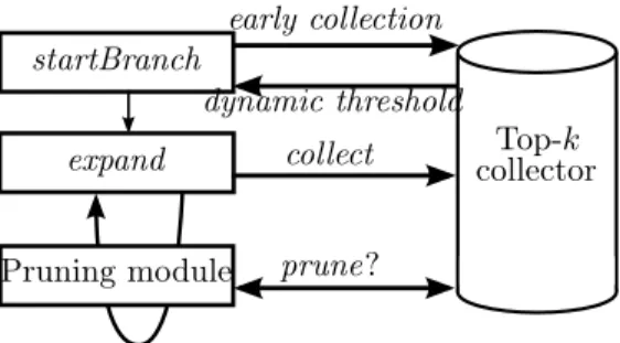
Figure 3: Overview of TopPI

3. TopPI algorithm

In this section, we present TopPI, an algorithm that solves the problem of finding the top-k closed itemsets (CIS) of each item.

3.1. Overview

TopPI is a recursive algorithm that follows the principles of CIS enumer-ation introduced in Section 2. The main functions of TopPI are presented in Algorithm 1, and Figure 3 provides an overview of TopPI. Then, we list the contributions of TopPI that are key to efficiently computing item-centric top-k CIS. Finally, we describe the main components of TopPI and indicate in which part of the algorithm each of these contributions operates.

3.1.1. Recursive structure

TopPI extracts CIS from a dataset D of transactions containing items from I. TopPI relies on closure extension operations and the definition of the first parent of CIS, presented in Section 2, to perform the CIS enumeration. The expand function builds CIS by extending a CIS P with an extension item e to obtain an new CIS Q ⊃ P . TopPI then recursively executes expand to extend Q with other items. This leads to a depth-first enumeration of CIS, where all supersets of Q containing items lower than e are enumerated, following the tree-shaped structure described in Section 2.

We describe the procedure performing the CIS enumeration following Algo-rithm 1. In this paragraph, we focus on the part of the algoAlgo-rithm that imple-ments the recursive algorithm. The details of TopPI are given in the remainder of Section 3. TopPI starts by executing startBranch on each item e of I (Line 3). The goal of this function is to enumerate all CISs present in the branch rooted at the singleton itemset {e}. TopPI enters the recursive expand function by extending the empty itemset (P = ∅) with e (Line 13). In expand , TopPI first computes Q, the closure of the union of an itemset P extended by e, to ensure that only closed itemsets are enumerated (Line 17). Furthermore, TopPI checks that hP, ei is the first parent of Q (Line 19) to avoid enumerating supersets of Q multiple times. When this test succeeds, TopPI performs recursive calls to expand (Line 21) to generate supersets of Q. All item present at least ε times

in DQ and smaller than e, based on the ordering of I, are potential extensions.

After these recursive calls, TopPI backtracks to P to enumerate siblings of Q. Once startBranch has been executed on all items of I, TopPI outputs the top-k of each item (Line 5) and terminates.

3.1.2. Contributions

The core recursive structure, inherited from LCM [4], provides TopPI with the basic ability to enumerate CISs. However, TopPI’s CIS enumeration strategy is significantly more complex than the one of traditional FIM algorithm.

TopPI aims at mining very large datasets while preserving their long-tailed distribution. FIM generally handles these cases by raising the frequency thresh-old ε, which allows the elimination of a large fraction of the data, to increase performance. With TopPI, we want to be able to output CIS appearing with very low frequency in the dataset. To this end, TopPI incorporates a dynamic threshold adjustment to improve performance without eliminating relevant data. Standard FIM algorithms rely on a simple pruning strategy to drastically reduce the number of CIS enumerated. Algorithms targeting the most frequent CIS, using a threshold or a global top-k, directly rely on the anti-monotony property of itemsets’ support [1]. Given two CISs P and Q, P ⊂ Q, if P is not a valid result, then Q isn’t one either, since support_D(P ) > support_D(Q). Hence, reaching a CIS whose support is too low to be a valid result means the early termination of a recursion, with the pruning of the sub-tree. This is, however, not applicable for TopPI: it is possible for the itemset {0, 1, 2} to be in the top-k of the item 0 while {1, 2} is not in the top-k of 1 or 2. This makes the early termination of the enumeration of a CIS branch harder to decide. TopPI introduces a new pruning strategy to tackle this issue.

Efficient top-k processing generally relies on the early discovery of high rank-ing results. This allows, usrank-ing heuristics, the prunrank-ing of large fractions of can-didates without having to perform their exact computation. TopPI boosts the efficiency of its pruning algorithm by introducing the early collection of promis-ing results, and optimizpromis-ing the order of CIS enumeration.

3.1.3. Components of TopPI

We now present the key components of TopPI in Figure 3. TopPI executes the startBranch function for each item and, as described in Section 3.1.1, re-cursively calls expand to enumerate CISs. In both these functions, TopPI takes advantage of an indexing of items by frequency to optimize the order of CIS enumeration. The top-k collector stores the results of TopPI by maintaining for each item the current version of its top-k CISs. TopPI transmits CISs to the collector using collect in expand , but also in startBranch with an early collec-tion of partial itemsets. Using the current status of the top-k of each item, the collector provides a dynamic support threshold at the beginning of each branch that allows TopPI to heavily compress the dataset without losing any potential result. The state of the collector is also used in expand through the prune func-tion to determine whether a recursive execufunc-tion may produce CISs part of the top-k of an item.

clo(∅) = ∅1 {0}, 172 3 {5}, 14 {0, 5}, 65 {1, 5}, 66 {0, 1, 5}, 57 {2, 3, 5}, 98 {2, 3, 5}, 99 10 h∅, 0i h∅, 1 . . . 4i h∅, 5i h∅, 6 . . . |I| − 1i h{5}, 0i h{5}, 1i h{1, 5}, 0i h{5}, 2i h{5}, 3i 4

(a) Example of CIS enumeration tree of TopPI. This figure focuses on the branches of items 0 and 5. hP, ii denotes the closure extension operation.

item top(i): P , support (P )

i 1st ₂nd ₃rd ₄th

0 {0}, 17 {0, 1}, 11 {0, 5}, 6 {0, 1, 5}, 5 5 {5}, 14 {2, 3, 5}, 9 {5, 6}, 8 {5, 9}, 7

(b) TopPI results for items 0 and 5 with k = 4 Figure 4: Illustration of TopPI’s execution

In order to help understanding the detailed explanations presented through-out Section 3, we provide a running example in Figure 4. For sake of simplicity, this example is not provided as a dataset and a complete execution trace. In-stead, Figure 4a represents a partial enumeration tree over an arbitrary dataset: only selected branches are presented (branches of items 0 and 5). However, these branches are sufficient to illustrate all optimizations of TopPI, as will be detailed later. Figure 4b also shows the end result of the algorithm for k = 4: the top-4 itemsets for items 0 and 5. This example will be used to illustrate the top-k collector, the optimized order of CIS enumeration, and the early collec-tion of partial itemsets in Seccollec-tion 3.2. It will serve as a basis to show how the current top-k results can be used to compute a dynamic support threshold in Section 3.3. Finally, it will support the description of TopPI’s pruning strategy in Section 3.4.

3.2. Enumeration and collection of closed itemsets 3.2.1. Top-k collector

TopPI aims at finding, for each item i in the dataset, the k CISs contain-ing i havcontain-ing the highest support. Similarly to traditional top-k processcontain-ing ap-proaches [8], TopPI relies on heap structures to update top-k results throughout the execution. TopPI’s top-k collector maintains, for each item i ∈ I, top(i ), a

Algorithm 2: Collector functions

1 Function collect (P , s, c)

Data: itemset P , its support s, boolean indicating whether P is closed c

Result: Updates appropriate top(i )

2 begin

3 foreach i ∈ P do

4 if |top(i )| < k ∨ entryThreshold (i ) < s then 5 if c ∧ ((P0, s, c0) ∈ top(i ), ∀P0⊆ P ) then 6 remove(top(i ), (P0, s, c0))

7 insert (top(i ), (P , s, c))

8 Function entryThreshold (i )

Data: item i

Result: the minimum support to enter the top-k of i

9 begin 10 if |top(i )| < k then 11 return 2 12 else 13 (P, s, c) ← last (top(i )) 14 if c then 15 return s 16 else 17 return s + 1

heap containing the current version of the top-k of i. Figure 4b shows top(0 ) and top(5 ) for the example execution of TopPI. top(i ) is sorted by decreasing support of CIS, and maintains a maximal size of k by automatically eliminating the lowest entry when its size exceeds k. Hence, at any point in time, a CIS can be added to top(i ) if its support is greater than the one of the last entry, or 2 if top(i ) contains less than k entries. The helper function entryThreshold (i ) in Algorithm 2 returns the support entry threshold of item i. In Figure 4b, entryThreshold (0 ) = 6 and entryThreshold (5 ) = 8. Upon computing the sup-port of an itemset P , TopPI updates top(i ) for all items i ∈ P using the collect function in Algorithm 1 (Line 18). Once the execution is complete, the results are known to be exact and are returned to the analyst (Algorithm 1, Line 5). The details of collect are given in Algorithm 2. Cases where c is false, and where the expression of Line 5 returns true are covered in Section 3.2.3.

As introduced in Section 3.1.2, TopPI implements a pruning strategy to avoid enumerating CIS and converge to the optimal results quickly. The details of the pruning strategy are presented in Section 3.4. As many top-k algorithms,

pruning in TopPI is most efficient when the entry threshold of each top(i ) heap is high. We now review two methods used by TopPI to collect CISs having a high support early in the execution.

3.2.2. Optimized enumeration order

Before mining a dataset, TopPI executes a pre-processing phase in which items are indexed by decreasing frequency. Hence, the most frequent item is indexed with 0 and the least frequent with |I| − 1. TopPI relies on this indexing when enumerating items (Algorithm 1, Lines 2 and 20). In the example of Figure 4a, the item indexed with 0 has a frequency of 17, so its branch 2 is enumerated before item 5 whose frequency is 14 4 . This method ensures that, for any item i ∈ I, the first itemsets containing i enumerated by TopPI combine i with some of the most frequent items in the dataset, which increases their probability of having a high support and raises entryThreshold (i ). Note that an additional side benefit is that this reduces the probability of failing a first-parent test (Line 19), which reduces computational overhead.

3.2.3. Early collection

TopPI focuses on mining closed itemsets to avoid redundant results. The canonical way to enumerate CISs, presented in Section 2.3, is a depth first approach combined with a first-parent definition to avoid enumerating the same CIS multiple times. While TopPI follows this general concept (Section 3.1.1), it introduces two key modifications.

TopPI computes the closure Q of an itemset P extended by e (Algorithm 1, Line 17). In the example execution of Figure 4a, clo({2, 5}) = clo({3, 5}) = {2, 3, 5}. Contrary to the standard approach, TopPI collects Q before perform-ing the first-parent test. Hence, while h{5}, 2i is not the first parent of {2, 3, 5}, {2, 3, 5} is collected at 8 . This allows TopPI to update the top(i ) heap of each item contained in Q as early as possible, and contributes to raising their entry thresholds. The drawback is that TopPI may enumerate Q multiple times (e.g. {2, 3, 5} is enumerated again at 9 ). This feature is undesirable when CISs are directly outputted upon their enumeration. However, TopPI only re-turns the results at the end of the enumeration. Duplicates are detected in the collect function (Algorithm 2, Line 5). Collecting a CIS as early as possible directly affects pruning potential and largely compensates the cost of duplicate detection.

Given a CIS P and an extension item e, TopPI has direct access to the support of P ∪ {e}, as it is pre-computed when generating DP. However,

com-puting Q, the closure of P ∪ {e}, is costly as it requires comcom-puting the support of all items in DP[{e}]. TopPI takes advantage of the availability of extension

support information to perform, at a negligible cost, a restricted breadth-first exploration. This operation takes place when starting a new branch of CIS enumeration for item e (Algorithm 1, Line 7): TopPI performs the early collec-tion of partial itemsets. These itemsets are partial because their closure has not been evaluated yet, and the top-k collector marks them with a special flag (third argument of collect set to false). In the example of Figure 4a, when starting

the branch of item 0 2 , TopPI builds D{0}. This allows the early collection

of 3 partial itemsets: {0, 1} with support 11, {0, 5} with support 6 and {0, 7} with support 4. The benefit of pre-filling top(e) with partial itemsets is that it significantly raises the entrance threshold of top(e). These partial items are later either ejected from top(e) by more (or equally) frequent closed itemsets, or replaced by their closed form upon its computation (Algorithm 2, Line 5). For instance, {0, 7} is replaced by {0, 1, 5} in top(0 ) at 7 since {0, 1, 5} has a higher support. Note that, if no additional verification was performed, this could lead to errors in the final version of top(i ). Indeed, two partial itemsets {i, j} and {i, l} of equal support may in fact be the same closed itemset {i, j, l}. Inserting both into top(e) occupies two of the k slots instead of one, which leads to an overestimation of the entrance threshold of top(e), and trigger the elimination of legitimate top-k CIS of e. Let’s consider the case of item 5 in Figure 4a 4 : in D{5}, items 2, 3 have a frequency of 9, 6 has a frequency of 8 and 9 has a

frequency of 7. If TopPI inserts the partial itemsets {2, 5}, {3, 5} and {5, 6} in top(5 ), entryThreshold (5 ) is raised to 8, which means that {5, 9} cannot enter top(5 ) because it’s support is 7. But the partial itemsets {2, 5} and {3, 5} are in fact a single closed itemset {2, 3, 5}, so the output of TopPI would not be correct if both were inserted. TopPI deals with this problem by only selecting partial itemsets with distinct supports (function topDistinctSupports in Algorithm 1). Hence TopPI does not risk inserting partial itemsets corresponding to the same closed itemset. So after 4 , entryThreshold (5 ) = 7 and the last entry of top(5 ) is the partial itemset {5, 9}.

3.3. Dynamic threshold adjustment

Each dataset, materialized in memory, is accessible through two data struc-tures: a horizontal and a vertical representation. The horizontal representation is transaction-based, and provides access, given a transaction index, to the set of items present in the transaction. Conversely, the vertical representation is item-based and provides, for each item, the list of transactions it belongs to. When executing the expand function, TopPI accesses DP[e] using the vertical

representation, to only read from DP the transactions that contain e. TopPI

then scans the transactions of DP[e], using the horizontal representation, to

compute the support of all items in DP[e]. Any item having the same support

as e is part of Q, the closure of P ∪ {e}, and is considered in the first parent test of Algorithm 1 Line 19. The supports of other items are used when executing the recursive calls to expand at the loop Line 20.

TopPI is designed to operate on datasets containing millions of items and transactions. Thus the initial dataset D typically occupies a few gigabytes, making support counting operations expensive. FIM algorithms generally rely on a high fixed frequency threshold, which allows them at start-up to eliminate from D all infrequent items. This considerably reduces the size of D but also eliminates the long tail of the dataset. Instead, to reduce execution-time while preserving very-low support itemsets, TopPI dynamically determines the appro-priate frequency threshold for each branch of the recursive CIS enumeration.

As explained in Section 2.3, when TopPI starts a CIS expansion branch (startBranch function) for an item e, the CIS recursively generated may only contain items smaller than e. TopPI makes use of this property (Algorithm 1, Line 9) to compute an appropriate support threshold value for the branch. TopPI queries the collector using entryThreshold (i ) to obtain the minimum entry threshold of the top-k of these items. The dynamic frequency threshold, εe, is set to the minimum of these entry threshold. For instance, in Figure 4a

4 , ε5is evaluated considering entryThreshold (i )∀i ∈ [0, 5]. If we ignore items 1

to 4, then ε5= 4 because, at this point of the execution, entryThreshold (0 ) = 4

(see partial itemset {0, 7} in Section 3.2.3) and entryThreshold (5 ) = 7. As an optimization, TopPI only considers in Line 11 items that have the potential to update their top-k in this branch, i.e. items whose support in D[{e}] is higher than their entry threshold. In expand , TopPI materializes in memory DQ, where

Q is the closure of e, using εeto reduce the size of the dataset as much as possible

while ensuring that no relevant CIS is lost. As the collector receives new CIS when recursively executing expand , the dynamic threshold could be updated to a higher value. However, it is most efficient to only perform this operation when starting a new branch, as it directly benefits from the early collection of partial itemsets (Section 3.2.3) and has a significant impact. Further adjustments in the same branch are not always amortized. Dynamic threshold adjustment combines particularly well with the frequency-based iteration order introduced in Section 3.2.2. Indeed, frequent items tend to have high entrance thresholds. 3.4. Pruning strategy

3.4.1. General concept

There are potentially 2|I|itemsets in a dataset, and TopPI targets datasets containing hundreds of thousands to millions of items. It is therefore crucial to provide TopPI with a pruning function able to eliminate a large fractions of the itemsets in order to obtain results in a reasonable time. TopPI relies on a tree-shaped enumeration of CIS, following a recursive approach. In this context, pruning consists in, given a current itemset P and an extension item e, deciding to not enumerate the 2|{i∈I\P,i<e}| itemsets present in this sub-tree.

In TopPI, the decision to prune is taken on Line 16 of Algorithm 1, at the beginning of the recursive expand function. As explained in Section 3.1.2, pruning is generally simple in standard FIM algorithms, thanks to the anti-monotony property of itemsets’ support. Whenever P ’s support is not high enough to be part of the results, given that no superset of P can have a higher support, the whole sub-tree can be safely eliminated. However, in TopPI, given a CIS Q with hP, ei as first parent, Q can be part of the top-k of item e while P is not part of the top-k of any item contained in P . For instance, in Figure 4, {0, 1, 5} is part of top(0 ) while its first parent itemset {1, 5} is not in top(5 ). Consequently, the tree traversed by TopPI is not monotonous, and TopPI has to go through CIS which are not part of the results to recursively reach some of the results. TopPI does not prune a sub-tree rooted at P based on P alone, but considers all the itemsets that could be recursively enumerated from P through

Algorithm 3: Pruning function

1 Function prune(P , e, DP, ε)

Data: itemset P , extension item e, reduced dataset DP, minimum

support threshold ε

Result: false if expand (P , e, DP, ε) may produce an itemset part of

the top-k of an extension item, true otherwise

2 begin

3 foreach i ∈ P ∪ {e} do

4 if supportDP({e})) ≥ entryThreshold (i )) then

5 return false

6 foreach i ∈ freq_ε(DP) | i < e ∧ i 6∈ P do // Potential future

extensions

7 boundi = min(supportDP({e}), supportDP({i }))

8 if boundi≥ entryThreshold (i ) then 9 P_exti←T_t∈D

P[{i}]t

10 if max (P_{ext i}) ≤ e then

11 return false

12 return true

first-parent closure extensions. We now detail the pruning strategy of TopPI (Algorithm 3).

3.4.2. Algorithmic design

TopPI implements a threshold algorithm based on the support of CIS simul-taneously over multiple top-k. The main difficulty is the fine-grained character-ization of which top-k can be affected by recursions of expand .

The prune function queries the collector using entryThreshold to determine whether Q = clo(P ∪ {e}), or any itemset recursively generated by expanding Q, can impact the top(i ) of any item i ∈ I. If this is not the case, then the sub-tree rooted at Q can be safely eliminated from the CIS enumeration without altering the completeness of TopPI’s results. We refer to the set of CIS present in this sub-tree rooted at Q as CQ. As explained in Section 2.3, the itemsets

of CQ all contain (i) e, the extension item, (ii) the items of P , the extended

itemset, and (iii) potentially any item inferior to e, to be added by closure or recursive extensions.

Cases (i) and (ii) are considered in Lines 3–5. The anti-monotony property ensures that, among the itemsets of CQ, Q has the highest support, equal to

supportDP({e}). Hence, we check this support against top(i ), ∀i ∈ P ∪ {e}.

Items belonging to case (iii) are the remaining items, included in the potential supersets of P ∪{e}. Their impact is evaluated in Lines 6–11. It is not possible to know the exact support of these supersets as they are not yet explored. However for the pruning operation, an upper bound is sufficient to determine if it is safe

to prune or not. This upper bound is shown in Line 7 and is the minimum between the support of e and i in the projected dataset DP. In the example

of Figure 4a, TopPI enumerates {0, 5} 5 which is added to top(0 ) (case (i)), replacing a partial itemset added during the early collection phase 2 . TopPI then enumerates {1, 5} 6 in order to reach {0, 1, 5} 7 . This is an instance of case (iii), as 0 is part of the items lower than 1 that can be recursively added. When extending {5} with 3 9 , top(5 ) already contains {2, 3, 5} 8 . However, TopPI still performs this operation to check whether some supersets of {2, 3, 5} are frequent enough to be included in top(5 ) (case (ii)). In our example, no item in D{2,3,5} is frequent enough, and TopPI backtracks.

One last property of the enumeration tree is exploited to further improve the pruning. When an item i passes the test of Line 8, normally prune should immediately return false, preventing pruning. However, it is not guaranteed that a CIS containing i will be actually reached by the enumeration, as a chain of first parent tests has to be verified to allow that. Line 9 therefore performs a closure on item i in DP. In Line 10, let p = max (clo(P ∪ {i })). If the item p

is lower or equal to e, then the first parent test may pass and it is not safe to prune. But if p is strictly greater than e, then it is sure that the CIS sub-tree created by expanding P with e will not produce any itemset containing i, as subsequent first parent tests will fail (Q will be found in C{p}). Hence, top(i )

cannot be considered for potential updates. This reasoning is formalized in the following theorem.

Theorem 1. Let P be a closed frequent itemset and e > i two items of I such that i 6∈ P , e 6∈ P .

Let Pext i=Tt∈DP[{i}]t = clo(P ∪{i}). If max (Pext i) > e, then expand (P, e, DP, ε)

does not output any itemset J ⊃ P such that i ∈ J .

Proof. Given that max(Pext i) > e, we can determine that ∃j ∈ Pext i such

that j > e and D[P ∪ {j}] ⊇ D[P ∪ {i}]. As J ⊃ P , and i ∈ J , by transitivity we have D[J ∪ {j}] = D[J ∪ {i}] = D[J ], and j is part of J . Hence, max (J \ P ) ≥ j. As TopPI only extends itemsets using items inferior to the previous extension, in this case e, and j > e, if expand(P, e, DP, ε) or one of its recursive calls

generates such an itemset J , it is aborted by the first parent test of Algorithm 1 in Line 19.

This last improvement allows to further increase the number of times when prune eliminates parts of the enumeration tree, leading to reduced execution times.

3.4.3. Optimizing pruning evaluation

For efficiency purposes, TopPI performs important optimizations in the im-plementation of the prune function.

The loops of Lines 3–5 and 6–11 of Algorithm 3 can iterate on up to |I| items, and thus take a significant amount of time to complete. To optimize the execution of the pruning function, we leverage the fact that TopPI enumerates

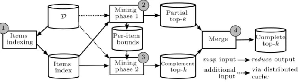
map input reduce output via distributed additional Items index Complement top-k Complete top-k Mining phase 1 2 Partial top-k Items indexing 1 Merge 4 Per-item bounds Mining phase 2 3 D input cache

Figure 5: Hadoop implementation of TopPI

extensions by increasing item order. Given two items e and f successive in the enumeration of the extensions of an itemset P (Algorithm 1, Line 20), the executions of prune(P, e, DP, ε) and prune(P, f, DP, ε) are extremely similar

(Algorithm 3). The loop of Lines 3–5 enumerates the items of P in both cases. As e < f , in the execution of prune(P, f, DP, ε), the loop of Lines 6–11 can

be divided into an iteration on i ∈ I | i < e ∧ i 6∈ P and an execution for i = e. Thus, the execution of prune(P, e, DP, ε) is a prefix of the execution

of prune(P, f, DP, ε). To take full advantage of this property, whenever prune

returns true, TopPI stores an upper bound on the extension support for which this result holds. For the following extension f , if support_DP(f ) is below this bound, it is safe to skip the loop of Lines 3–5 as well as the prefix of the loop of lines 6–11, significantly reducing the execution time of prune. Lines 9–10 cause rare exceptions to this rule, which are correctly handled by TopPI using an additional flag.

In the loop of lines 6–11, the computation of the closure in line 10 is an expensive operation. Similarly to our previous optimization, given an execution prune(P, f, DP, ε), for any item i considered in this loop expand (P , i , DP, ε) has

been executed previously, as i < e. Hence, this closure has in fact already been computed in line 17 of Algorithm 1, and TopPI can reuse this result. This is the reason why we perform the closure of P ∪ {i} and not of P ∪ {e, i}, which would be more precise but is not pre-computed.

4. Scaling TopPI

We first present the multithreaded version of TopPI, designed to take full advantage of the multi-core CPUs available on servers. Then, to scale beyond the capacity of a single server, we present a distributed version of TopPI designed for MapReduce [9]. The goal is to divide the mining process into independent subtasks executed on workers while (i) ensuring the output completeness, (ii) avoiding redundant computation, and (iii) maintaining pruning performance. 4.1. Shared-memory TopPI

The enumeration of CISs by TopPI follows a tree structure, described in Sec-tion 2.3. As shown by Négrevergne et al. [10], such enumeraSec-tion can be adapted

to shared-memory parallel systems by dispatching branches (i.e. startBranch invocations, Algorithm 1, Line 3) to different threads. This policy ensures that reduced datasets materialized in memory by a thread are accessed by the same thread, which improves memory locality in NUMA architectures and makes bet-ter use of CPU caches. Some branches of the enumeration can generate much more CISs than others. Towards the end of the execution, when a thread finishes the exploration of a branch and no new branch needs to be explored, TopPI re-lies a work stealing policy to split the recursions of expand over multiple threads. Threads take into account the NUMA topology to prioritize stealing from other threads that share caches or are on the same socket.

The top-k collector is shared between threads using fine-grained locks for the top-k of each item. In its single threaded version, TopPI always collects partial itemsets before replacing them with their closed form (Section 3.2.3). This is no longer the case in a parallel environment, so the collect function in Algorithm 2 must be updated to avoid inserting a partial (c = false) itemsets P when P0, a superset of P having the same support, is already present.

4.2. Distributed TopPI

When executing TopPI on a cluster of workers, each worker executes one instance of the multi-threaded version of TopPI described in Section 4.1. We rely on Hadoop to distribute the execution over all workers in parallel. We first describe how the enumeration of CISs is split between the workers, and then describe a two-phase mining approach designed to reduce distribution overhead. Figure 5 gives an overview of our solution.

4.2.1. Partitioning the CISs enumeration

In a distributed setting, enumeration branches are dispatched among work-ers. Each worker is assigned a partition of items G ⊆ I, and restricts its explo-ration to the branches starting with an element of G (Algorithm 1, Line 2). Fol-lowing the example of Table 2, a worker that is assigned the partition G = {0, 2} outputs the itemsets {0},{2} and {0, 1, 2}. TopPI’s closure extensions follow a strictly decreasing item order, so a worker generates itemsets P such that max (P ) ∈ G. Thus, all workers generate different itemsets, without overlap nor need for a synchronization among them. This partitioning ensures that CISs are only generated once, so that no processing time is wasted executing redundant operations.

Given the restrictions on the enumeration tree, a worker only requires the transactions of D containing items of its partition G. In Section 3.2.2, we de-scribe the pre-processing step of TopPI in which items are indexed by decreasing frequency. Workers must agree on the ordering of items as it determines the first parent of a CIS. Should two tasks obtain a different assignment of items identifiers, several CISs would be generated multiple times, and others would be lacking in the output. Consequently, indexing items by decreasing frequency is performed jointly by all workers on the original dataset D (Figure 5 1 ). Once the items have been sorted by frequency and indexed, they are assigned

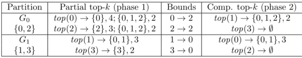
Partition Partial top-k (phase 1) Bounds Comp. top-k (phase 2) G0 top(0) → {0}, 4; {0, 1, 2}, 2 0 → 2 top(1) → {0, 1, 2}, 2

{0, 2} top(2) → {2}, 3; {0, 1, 2}, 2 2 → 2 top(3) → ∅ G1 top(1) → {0, 1}, 3 1 → 0 top(0) → {0, 1}, 3

{1, 3} top(3) → {3}, 2 3 → 0 top(2) → ∅

Table 3: 2-phase mining over the sample database (Table 2a) with 2 workers, k = 2. to groups in a round robin fashion. This ensures that the most frequent items, which form the largest reduced datasets, are assigned to different groups, which balances the load of workers.

4.2.2. Two-phase mining

The partitioning of the enumeration tree introduces the drawback that the top-k CISs of an item may be generated by any worker, without the possibility of predicting which ones. A naive solution is for each worker to compute a local top-k for all items, and then merge all local top-k into the exact top-k. This requires enumerating up to k × |I| CISs per worker, exploring a much larger fraction of the CIS space than centralized TopPI, and significantly limiting the scalability.

Instead, we rely on the following idea: given an item i ∈ G, the worker re-sponsible for G collects a partial version of top(i ) close to the complete one. In-deed, as described in Section 3.2.2, it generates CISs that combine i with smaller items of the dataset (i.e. more frequent items, thanks the pre-processing). Even though these may not all be in the actual top-k CISs of i, they are likely to have high support. Consequently, we run distributed TopPI as a two-phase mining process. In the first phase (Figure 5 2 ), the worker only collects itemsets for items i ∈ G. This step outputs a first partial version of each item’s top-k, as well as a lower bound on the support of their complete top-k. In the second phase (Figure 5 3 ), the worker only collects itemsets for items i 6∈ G to generate the complement top-k. A final MapReduce job is executed to merge the partial top-k and the complement top-k (Figure 5 4 ). We illustrate this process with the example in Table 3.

Overall, this two-phase process is scalable. The first phase of mining com-pletely splits the enumeration and the collection among groups, without any impact on the accuracy of pruning. If we compare it to the naive version, we can see that the second phase is the exact complement of phase one, to overall achieve the same task. Even though the second phase apparently suffers from the same scalability problem as the naive version, the bounds generated at phase one ensure that this mining phase is extremely short and accurately targeted to simply complete the results of phase one. We confirm the overall scalability of two-phase TopPI in Section 5.3.2.

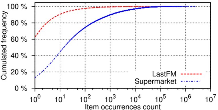
0 % 20 % 40 % 60 % 80 % 100 % 100 101 102 103 104 105 106 107 Cumulated frequency

Item occurrences count LastFM Supermarket

Figure 6: Cumulative frequency of items in our two datasets.

5. Performance evaluation

We evaluate TopPI with two real-life datasets on a multi-core machine and a Hadoop cluster. Our complete setup is described in Section 5.1. We evaluate TopPI on a multi-core machine in Section 5.2. We first compare TopPI against multiple baselines, and evaluate its scalability. We then consider the case of a Hadoop cluster in Section 5.3, and evaluate TopPI against its closest competitor on this platform, PFP [2].

5.1. Experimental setup We use 2 real datasets:

• Supermarket is a 2.8GB retail basket dataset collected from 87 supermar-kets over 27 months. There are 54.8 million transactions and 389,372 items.

• LastFM is a music recommendation website, on which we crawled 1.2 million public profile pages. Each transaction contains the 50 favorite artists of a user. We found 1.2 million different artists and the input file weights 277MB. This dataset is available1.

As shown by Figure 6, both datasets have a long tail distribution: the ma-jority of items occur in less than a hundred transactions. This is even more pronounced for LastFM, where only 450,399 items out of the 1.2 million avail-able occur two times or more.

Our two hardware settings will be referred to as server and cluster. The multi-threaded variant of TopPI runs on the server configuration: a single ma-chine containing 4 Intel Xeon X7560 8-cores CPUs, for a total of 32 cores, and 64 GB of RAM. Hadoop programs (TopPI and PFP) are deployed on the clus-ter configuration, which consists of up to 51 machines running Hadoop 1.2.1

(without speculative execution), one of them acting as the master node. Each machine contains 2 Intel Xeon E5520 4-cores CPUs and 24 GB of RAM. We implemented TopPI in Java and its source code is available2. All measurements presented here are averages of 3 consecutive runs.

5.2. Single server

We consider two baseline algorithms that could be used to mine item-centric CIS. The first one, in Section 5.2.1, is a standard threshold-based frequent item-set mining algorithm that computes top-k CIS as a post-processing. Then, in Section 5.2.1, we consider the case of a global top-k algorithm executed re-peatedly for each item. We validate the impact of TopPI’s optimizations in Section 5.2.3. In Section 5.2.4 we measure TopPI’s resource utilization and scalability.

5.2.1. Frequency threshold baseline

In this preliminary experiment, we consider a standard CIS mining algorithm as a baseline. Given a frequency threshold ε, the algorithm extracts all CIS whose support is above ε. The top-k CIS of each item can then be computed as a post-processing on these results, thus producing the same output as TopPI. We evaluate this approach for different frequency thresholds ε and present the results in Figure 7. This post-processing approach does not take the number of desired CIS per item k as a parameter. Hence, we instead measure for each value of ε the number of items appearing in at least k CIS for 3 values of k.

Each item is present in a CIS whose support is equal to the frequency of the item in the dataset. This CIS, a singleton in most cases, is the only result selected when k = 1. We already notice that, given the long-tailed distribution of the data, is is necessary to reach very low values of ε to select a large number of items. In the case of LastFM, only 2% of the items appear in more than 0.01% of the transactions. Furthermore, for the same value of ε, only 1% of the items are included in more than 10 frequent CIS. In practice, it takes 150 hours of CPU time to extract all CIS for this support threshold. The algorithm mines over 2 billions CIS, but only 24,536 items out of 1.2 million appear in these results. The behavior of this approach on Supermarket, although slightly better, highlights the same limitations. Using a frequency threshold of 10−5%, mining frequent CIS takes one hour. This may appear to be a reasonable run-time, but the results are not very useful for the analysts: the 34,151,639 CIS only contain a minority of the available products, 90% of the items are in less than 10 CIS.

As this experiment shows, standard CIS mining algorithms are perfectly capable of efficiently enumerating billions of CIS. The problem is that these itemsets only contain the most frequent items in the dataset, and fail to cover items from the long tail. Hence, the post-processing approach spends most of the mining time generating an overwhelming amount of CIS which are of no

0 %

5 %

10 %

15 %

20 %

25 %

30 %

0.0001 %

0.001 %

0.01 %

Items having k freq. itemsets

Relative frequency threshold

k=1

k=10

k=50

0 %

0.5 %

1 %

1.5 %

2 %

2.5 %

0.01 %

0.1 %

1 %

Items having k freq. itemsets

Relative frequency threshold

k=1

k=10

k=50

(b) LastFM

Figure 7: Proportion of available items appearing in at least k itemsets (for k ∈ {1, 10, 50}), using frequent CIS mining, with respect to the frequency threshold.

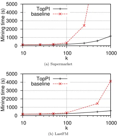
0

1000

2000

3000

4000

5000

10

100

1000

Mining time (s)

k

TopPI

baseline

0

1000

2000

3000

4000

5000

10

100

1000

Mining time (s)

k

TopPI

baseline

Figure 8: TopPI and global top-k baseline runtimes (in seconds), using 32 threads

interest to the analysts. This observation motivated the development of TopPI, that efficiently computes item-centric CIS using an integrated approach. 5.2.2. Top-k baseline

We now by compare TopPI to a top-k baseline, which is the most straight-forward solution to our problem statement: given the parameter k, the baseline applies a global top-k CIS mining algorithm on the projected dataset D[i], for each item i in D occurring at least twice.

To perform this experiment, we implemented TFP[5] to serve as the top-k miner. TFP has an additional parameter lmin, which is the minimal itemset

size. In our case lmin is always equal to 1 so we added a major pre-filtering:

∀i, when projecting i on D, we keep only the items having one of the k highest supports in D[i]. In other words, the baseline also benefits from a dynamic threshold adjustment. This is essential to its ability to mine a dataset like Su-permarket. The baseline also benefits from the occurrence delivery provided by our input dataset implementation (i.e. instant access to D[i]). Its parallelization is straightforward, hence both solutions use 32 threads, the maximum allowed on server.

0

1e+07

2e+07

3e+07

4e+07

5e+07

6e+07

0

20

40

60

80

100

#itemsets

k

Outputted

Enum. by TopPI

Enum. by baseline

0

1e+07

2e+07

3e+07

4e+07

5e+07

0

20

40

60

80

100

#itemsets

k

Outputted

Enum. by TopPI

Enum. by baseline

Figure 9: Number of useful CIS vs. CIS enumerated

Figure 8 shows the runtimes on our datasets when varying k. TopPI sig-nificantly outperforms its baseline, which fails to output results in some cases (taking over 8 hours to complete or running out of memory). Despite having around 40 times more transactions than LastFM, Supermarket is mined very efficiently.

The execution time of TopPI increases slightly super-linearly with k. This behavior is common in top-k algorithms. The size of the output is proportional to k, which suggests a linear behavior. However, as k increases, the difference between the kth _{best result and the following ones tends to diminish. Thus,}

pruning is not as efficient and extra verifications need to be performed, leading to a super-linear execution time.

To better understand the performance difference between TopPI and the baseline, we trace the execution of each algorithm to evaluate the number of itemsets enumerated. Figure 9 reports this result, and compares it to the num-ber of itemsets actually present in the output. Ideally, the algorithm should only enumerate outputted solutions. As explained in Section 3, the problem of finding top-k itemsets for each item is not anti-monotone, and TopPI has to enumerate a few additional itemsets to reach some solutions. Thanks the the

Dataset Complete W/o optimized W/o dynamic W/o TopPI pruning threshold adjustment both

LastFM 252 307 304 374

Supermarket 275 3697 423 4072

Table 4: TopPI run-times (in seconds) on our datasets, using our machine’s full capacity (31 threads) and k = 250, when we disable the operations proposed in Section 3.

use of appropriate heuristics to guide the exploration, TopPI only enumerates a small fraction of discarded itemsets, which explains its good performance. On the contrary, TFP enumerates a significant amount of itemsets that do not con-tribute to the output. The main reason is that TFP does not perform closure extensions, but merges enumerated itemsets into their closure. When mining high support itemsets, which is the case in a global top-k context, this does not constitute a major problem, as the number of itemsets and closed itemsets are relatively close. However, at lower thresholds, each closed itemset can have hundreds of unclosed forms, which explains the poor performance of TFP in this experiment.

5.2.3. Impact of TopPI’s optimizations

In this experiment we measure the impact of optimizations included in TopPI’s algorithm (Section 3). To do so, we make these features optional in TopPI’s implementation, and evaluate their impact on the execution time. In particular, we evaluate the benefits of the optimized pruning evaluation (Sec-tion 3.4.3) and the dynamic threshold adjustment in startBranch (Sec(Sec-tion 3.3). Table 4 compares the execution time of these variants against the fully opti-mized version of TopPI’s, on all our datasets when using the full capacity of our server. We use k = 250, which is representative of our use cases and guarantees the interestingness of results (see Section 6.3). Disabling dynamic threshold ad-justment implies that all projected datasets created during the CIS exploration carry more items. Hence intermediate datasets are bigger. This slows down the exploration (+20% for LastFM, +53% for Supermarket) but also increase the memory consumption. The TFP-based baseline presented in the previous experiment cannot run without dynamic threshold adjustment, but TopPI still shows a reasonable run-time. When we also disable the use of a short-cut in the loops of the prune function, it becomes a major time consumer because it has to evaluate many extensions in Algorithm 3, lines 6–11. Without these opti-mizations TopPI is 48% slower on LastFM and 15 times slower on Supermarket. This experiment shows that it’s the combined usage of these optimizations that allows TopPI to mine large datasets efficiently.

5.2.4. Speedup on shared-memory systems

We conclude our evaluation of the centralized version of TopPI by reporting the mining time speedup with respect to the number of mining threads, in Figure 10. This measure uses up to 31 threads, leaving one core for the system.

0 8 16 24 0 4 8 12 16 20 24 28 32 Speedup #Threads Supermarket, k=50 LastFM, k=50 Linear

Figure 10: TopPI speedup on a single server

Our results show that, in practice, the allocation of more worker threads speeds up the mining process on the server configuration. On these datasets TopPI threads compete for memory accesses when building their reduced datasets. This important operation, performed at each step of the solutions traversal, trig-gers massive accesses to non-consecutive areas of the memory. Thus, when using 16 threads or more, the memory bus starts to become a bottleneck.

When 31 threads are used in parallel, 31 branches of the CIS tree are explored simultaneously and therefore held in memory, with the corresponding reduced datasets. Though, even with 32 threads, the peak memory usage of TopPI re-mains below 10 gigabytes for all datasets. This is shown by on Figures 11a and 11b, where we report TopPI’s peak RAM consumption for LastFM and Su-permarket respectively. As k grows, the top-k collector is expanded accordingly. Furthermore, the prune function guides TopPI towards deeper tree explorations to generate additional itemsets, thus keeping more reduced datasets in memory. These results demonstrate that TopPI is fast and scalable. Even on common hardware, TopPI is able to mine LastFM with k = 50 and ε = 2 on a laptop with 4 threads (Intel Core i7-3687U) and 6 GB of RAM in 16 minutes, while this operation takes 13 minutes for PFP on our cluster configuration with 200 cores (as presented in Section 5.3.1).

5.3. TopPI over Hadoop

5.3.1. Performance comparison to PFP

We now compare our Hadoop variant to PFP [2], the closest algorithm to TopPI: it returns, for each item, at most k frequent itemsets containing that item. We use the implementation available in the Apache Mahout Library [11]. We use 50 worker machines and launch 4 tasks per machine, allocating 5GB of memory to each. As PFP is not multithreaded, TopPI now uses a single thread per task. Mahout’s documentation recommends to create one task for every 20 to 30 items, thus PFP runs 20,000 tasks on LastFM and 17,000 on Supermarket. The measured runtimes are presented in Figure 12.

0

1

2

3

4

5

6

0

100

200

300

400

500

Peak RAM usage (GB)

k

6

7

8

9

10

0

100

200

300

400

500

Peak RAM usage (GB)

k

Figure 11: TopPI peak memory usage, using 32 threads

On Supermarket, PFP’s runtime is surprisingly uncorrelated to k. PFP can also not terminate correctly above k ≥ 1000 (TopPI can still run with k ≥ 2000). This may be caused by an implementation corner case, or by the difference between the two algorithms’ problem statements - TopPI provides stronger guarantees on long tail itemsets. This is further discussed in Section 6.1. On LastFM, increasing the value of k has only a moderate influence on TopPI’s runtime because, when distributed among 200 tasks, the mining phases are very short so the reported execution time mostly consists of Hadoop I/O. TopPI remains 3 to 4 times faster that PFP.

5.3.2. TopPI speedup

Figure 13 shows the speedup gained by the addition of worker nodes, on our biggest dataset, Supermarket, when k = 1000. Here we execute a single mining task per machine, which fully exploits the available resources by running 8 threads in all the available memory, 24GB.

TopPI shows a perfect speedup from 1 to 8 machines (64 cores), and steadily gets faster with the addition of workers. Overall, the total CPU time (summed

0

200

400

600

800

1000

0

100

200

300

400

500

Time (seconds)

k

PFP

TopPI

0

500

1000

1500

2000

2500

0

100

200

300

400

500

Time (seconds)

k

TopPI

PFP

Figure 12: TopPI and PFP runtimes on a 200-tasks Hadoop cluster

over all machines) spent in the mining phases (expand function) remains stable: from 35,000 seconds on average from 1 to 8 machines, it only raises to 38,500 seconds with 48 machines (using their 384 cores). Adding a task to TopPI incurs I/O costs, such as the time spent reading the initial dataset. Hence there is a trade-off between the execution time of the mining phases and the I/O overhead. In this configuration, the sweet spot is around 8 tasks. Should the workload increases, TopPI would achieve optimal speedup on larger clusters, as the overall mining time increases and compensates the I/O costs.

This validates the distribution strategy used for the mining phases: the load is well partitioned and does not increase significantly with the number of tasks.

6. Qualitative study

So far, we showed that ranking item-centric itemsets by support allows an efficient traversal of the solution space. In this section, we confirm that this ranking also highlights interesting patterns about long-tailed items. We also conduct a user study with marketing experts and learn that ranking itemsets in retail, by p-value, is superior to other measures. We use that to show that

0 16 32 48 0 16 32 48 Speedup #Machines Linear TopPI

Figure 13: TopPI speedup when running on Hadoop with on Supermarket (k = 1000)

the results of TopPI can be re-ranked using p-value and obtain useful results for analysts in the retail industry.

6.1. Mining the long tail

Figure 14 shows the average number of itemsets returned for each item, with respect to its frequency. In order to make these measures readable, we average them over item frequency intervals. For the least frequent items, neither TopPI nor PFP manages to output the requested k itemsets. This is expected as an item of frequency 3, for example, can be part of at most 4 CIS. For these items, PFP returns more itemsets than TopPI on LastFM, but most of them are redundant - both algorithms give the same number of closed itemsets. As item frequency increases, TopPI returns more itemsets, with almost filled top-k heaps for all items appearing at least 10 times in the dataset. PFP, however, is unable to find these itemsets and only returns close to k itemsets for items whose frequency is above 1000. The difference is even more striking on Supermarket, where PFP provides the required k itemsets per item only for items occurring more than 10,000 times.

These results show that, unlike PFP, TopPI performs a complete top-k CIS mining for all items, even ones in the long tail.

6.2. Example itemsets

From Supermarket:. Itemsets with high support can be found for very common products, such as milk: “milk, puff pastry” (10,315 occurrences), “milk, eggs” (9184) and “milk, cereals” (1237). Although this particular milk product was bought 274,196 times (i.e. in 0.5% of the transactions), some of its top-50 associated patterns would already be out of reach of traditional CIS algorithms: “milk, cereals” appears in 0.0022% transactions.

Interesting itemsets can also be found for less frequent (tail) products. For example, “frangipane, puff pastry, sugar” (522), shows the basic ingredients for french king cake. We also found evidence of some sushi parties, with itemsets such as “nori seaweed, wasabi, sushi rice, soy sauce” (133).

0

10

20

30

40

50

60

10

10

10

10

10

10

10

#itemsets in top(i)

support(i)

k

TopPI

PFP

0

10

20

30

40

50

60

10

10

10

10

10

10

10

#itemsets in top(i)

support(i)

k

TopPI

PFP

Figure 14: Average |top(i)| per item w.r.t. supportD(i) (k = 50)

From LastFM:. TopPI finds itemsets grouping artists of the same music genre. For example, the itemset “Tryo, La Rue Ketanou, Louise Attaque” (789 oc-currences), represents 3 french alternative bands. Among the top-10 CIS that contain “Vardoger” (a black-metal band from Norway which only occurs 10 times), we get the itemset “Vardoger, Antestor, Slechtvalk, Pantokrator, Crim-son Moonlight” (6 occurrences). TopPI often finds such itemsets, which, in the case of unknown artists, are particularly interesting to discover similar bands. 6.3. Ranking by p-value

While TopPI returns valuable results, its output also contains a few less in-teresting itemsets. TopPI focuses on support (recall) to select the top-k results of an item, but other aspects such as confidence (precision) are equally impor-tant. The traditional approach to mining itemsets with both high support and confidence is to first extract frequent itemsets, and filter them using a confidence threshold [1]. This method can be directly applied on the results of TopPI to obtain item-centric association rules.