ÉCOLE DE TECHNOLOGIE SUPÉRIEURE UNIVERSITÉ DU QUÉBEC
MANUSCRIPT-BASED THESIS PRESENTED TO ÉCOLE DE TECHNOLOGIE SUPÉRIEURE
IN PARTIAL FULFILLMENT OF THE REQUIREMENTS FOR A MASTER’S DEGREE WITH THESIS IN RENEWABLE ENERGY
AND ENERGY EFFICIENCY M.A.Sc.
BY
Tuesman CASTILLO CALVAS
OPTIMAL LOCATION AND COORDINATED VOLTAGE CONTROL FOR DISTRIBUTED GENERATORS IN DISTRIBUTION NETWORKS
MONTREAL, "JULY 19, 2016"
This Creative Commons license allows readers to download this work and share it with others as long as the author is credited. The content of this work cannot be modified in any way or used commercially.
BOARD OF EXAMINERS THIS THESIS HAS BEEN EVALUATED BY THE FOLLOWING BOARD OF EXAMINERS:
Prof. Maarouf Saad, thesis director
Département de génie électrique, École de technologie supérieure
Prof. Ambrish Chandra, President of the Jury
Département de génie électrique, École de technologie supérieure
Prof. Pierre-Jean Lagacé, Member of the Jury
Département de génie électrique, École de technologie supérieure
THIS THESIS WAS PRESENTED AND DEFENDED
IN THE PRESENCE OF A BOARD OF EXAMINERS AND THE PUBLIC ON "JUNE 20, 2016"
ACKNOWLEDGEMENTS
I would like to express my deep gratitude to my research director, Dr. Maarouf Saad, Départe-ment de génie électrique, ETS, for his guidance, support and advice towards the developed of my Master program and this thesis.
My sincere thanks to my colleges, Raul Castro and Byron Maza for their valuable suggestions and constructive criticism in my studies.
I would also like to acknowledge Secretaria de Educación Superior, Ciencia, Tecnología e Innovación (SENESCYT), for the financial support for my studies.
Finally, I wish to thank my parents, my sisters and my fiancée for their support and encourage-ment throughout my studies.
EMPLACEMENT OPTIMAL ET CONTRÔLE DE TENSION COORDONNÉ POUR LA GÉNÉRATION DISTRIBUÉE DANS LES RÉSEAUX ÉLECTRIQUES
Tuesman CASTILLO CALVAS RÉSUMÉ
Les générations distribuées (DGs) connectées aux réseaux de distribution sont de plus en plus populaires. Elles peuvent être utilisées comme un moyen pour réduire les impacts environ-nementaux de la production d’énergie. Toutefois, en dépit des multiples avantages que la DG apporte au réseau, une mauvaise planification et un mauvais fonctionnement peuvent conduire à des effets négatifs sur les réseaux de distribution. Une augmentation des pertes de puissance, un problème de stabilité de tension et un fonctionnement déficient de l’équipement de com-mande sont trois des principaux impacts qu’une mauvaise intégration d’un DG peut apporter au réseau. Pour compenser ces effets négatifs, ce mémoire propose une approche pour trouver l’emplacement et le dimensionnement optimaux de l’intégration de nouvelles DG au réseau tout en réduisant les pertes de puissance et en améliorant le profil de tension. De plus, un con-trôle de tension coordonné est présenté pour trouver le réglage optimal des puissances active et réactive de la DG. Ceci est obtenu en coordination avec des transformateurs avec changeurs de prise (OLTC) et des condensateurs shunt (SCs). Ce problème est formulé comme un problème d’optimisation multiobjectif résolu en utilisant les algorithmes génétiques (GA). Les méthodes proposées sont validées sur des réseaux de distribution triphasés déséquilibrés. De plus, des profils de charge et de production dynamiques ont été considérés.
Mots clés: Génération distribuée (DG), Intégration des DGs, Algorithmes génétiques, Con-trôle de tension, ConCon-trôle de tension coordonnée
OPTIMAL LOCATION AND COORDINATED VOLTAGE CONTROL FOR DISTRIBUTED GENERATORS IN DISTRIBUTION NETWORKS
Tuesman CASTILLO CALVAS ABSTRACT
Distributed Generators (DGs) connected to distribution networks are growing in popularity and as a feasible way to reduce environmental impacts in energy production. However, despite the multiple benefits that DG brings to the network, improper planning and operation of DG may lead to negative impacts into distribution networks. Increment in power losses, voltage instability, and deficient operation of control equipment are three of the main impacts that DG may bring to system. In order to revert the negative impacts of DG, this study proposes a method to find the optimal location and size of new DG units, reducing the power losses and enhancing the voltage profile. Also a coordinated voltage control method is presented in order to find the optimal setting for active and reactive power from DG, in coordination with the on-load tap changer (OLTC) and shunt capacitors (SCs). This study presents the multiobjective problem for both methods solved using a genetic algorithm (GA) technique. The proposed methods are tested with unbalance distribution networks. Additionally, the use of a time varying load and generation profile are considered.
Keywords: Distributed Generation, DG integration, Genetic algorithm, Voltage control, co-ordinated voltage control.
CONTENTS
Page
INTRODUCTION . . . 1
CHAPTER 1 LITERATURE REVIEW . . . 5
1.1 Introduction . . . 5
1.2 Impacts of Distributed Generation on distribution networks . . . 6
1.3 Literature Review on Distributed Generation Allocation . . . 7
1.4 Literature review on Coordinated Voltage control methods with Distributed Generation . . . 10
CHAPTER 2 DISTRIBUTION NETWORK MODELING WITH OPENDSS . . . 15
2.1 OpenDSS . . . 15
2.2 Simulation of a Medium Voltage Network with OpenDSS. . . 18
2.2.1 New Circuit . . . 18 2.2.2 Transformer . . . 19 2.2.3 Lines . . . 19 2.2.4 Loads . . . 20 2.2.5 Control Modes . . . 21 2.2.6 Solution Modes . . . 21
2.2.7 Monitors and Meters . . . 21
2.2.8 Simulation of a 13-node distribution network. . . 22
2.3 Co-simulation OpenDSS with Matlab . . . 25
2.4 OpenDSS-MATLAB initiation . . . 26
2.4.1 Load Shapes . . . 27
2.4.2 Photovoltaic system simulation . . . 27
2.4.2.1 Inverter Control . . . 28
2.4.3 Simulation and results . . . 29
CHAPTER 3 DISTRIBUTED GENERATION TECHNOLOGIES . . . 33
3.1 Introduction . . . 33
3.2 Combustion Engines . . . 33
3.2.1 Internal Combustion Engines . . . 33
3.2.2 Gas Combustion Turbines . . . 34
3.2.3 Micro-turbines . . . 34
3.2.4 Combined Heat and Power . . . 34
3.3 Fuel Cells . . . 35 3.4 Storage Devices . . . 35 3.4.1 Flywheels . . . 36 3.4.2 Batteries . . . 36 3.5 Renewables . . . 37 3.5.1 Photovoltaic generators . . . 37
XII
3.5.2 Wind Turbine generators . . . 38
3.5.3 Geothermal generators . . . 39
3.5.4 Small Hydropower . . . 39
CHAPTER 4 OPTIMAL LOCATION AND SIZE FOR VARIOUS RENEWABLE GENERATORS UNITS IN DISTRIBUTION NETWORKS . . . 41
4.1 Introduction . . . 41
4.2 Problem formulation . . . 44
4.2.1 Proposed methodology . . . 45
4.2.2 Genetic Algorithm . . . 48
4.3 Probabilistic Simulation . . . 48
4.3.1 Probabilistic Photovoltaic generator Model . . . 49
4.3.2 Probabilistic Load Model . . . 50
4.4 Solution Algorithm . . . 50
4.5 Test Systems and Verification . . . 51
4.5.1 Case studies: . . . 53 4.5.2 Simulation Results: . . . 55 4.5.2.1 Case1 . . . 55 4.5.2.2 Case 2 . . . 58 4.5.2.3 Case 3 . . . 58 4.5.2.4 Case 4 . . . 61 4.5.3 Energy losses . . . 62 4.6 Conclusion . . . 62
CHAPTER 5 COORDINATED VOLTAGE CONTROL FOR DISTRIBUTION NETWORKS WITH DISTRIBUTED GENERATION PARTICIPATION . . . 67
5.1 Introduction . . . 67
5.2 Problem Formulation . . . 71
5.2.1 Optimization problem formulation . . . 71
5.3 Case Study . . . 76
5.3.1 GA implementation . . . 76
5.3.2 Simulation test system 1 . . . 76
5.4 Simulation Results . . . 78
5.4.1 Impact on the total circuit power losses by applying the CVC method . . . 78
5.4.2 Impact of applying the CVC method on the voltage regulation . . . 79
5.5 Simulation test system 2 . . . 81
5.5.1 Results . . . 83
5.5.1.1 Impact on the total circuit power losses by applying the CVC method . . . 83
5.5.1.2 Impact of applying the CVC method on the voltage profile . . . 84
XIII
5.5.1.3 Impact on the OLTC and capacitor operations by
applying the CVC method . . . 84
5.6 Conclusion . . . 85
GENERAL CONCLUSION . . . 87
APPENDIX I OPENDSS CODE FOR THE IEEE 13 NODE TEST FEEDER . . . 89
APPENDIX II MATLAB CODE FOR PV INCLUSION AND VOLT/VAR CONTROL . . . 95
APPENDIX III OPTIMAL ALLOCATION ALGORITHM MATLAB CODE . . . .101
APPENDIX IV COORDINATED VOLTAGE CONTROL ALGORITHM MATLAB CODE . . . .105
LIST OF TABLES
Page Table 4.1 GA Parameters . . . 48 Table 4.2 Results for optimal DG location and sizing using GA and PSO
algorithm . . . 56 Table 4.3 Results of DG location and sizing for 4 DG units, case 1, 37-node
test feeder . . . 56 Table 4.4 Results of DG location and sizing for 4 DG units, case 2, 123-node
test feeder . . . 58 Table 4.5 Results compared with RLF method . . . 58 Table 4.6 Energy losses comparison and DG capacity for 24 hours period . . . 60 Table 4.7 DG allocation for 4 DG units, case 4, 37-node test feeder, 1-year
prediction. . . 61 Table 4.8 Maximum capacity and PF for 4 DG connections . . . 62 Table 5.1 Cumulative voltage deviation (CVD) and Power Losses for the
LIST OF FIGURES
Page
Figure 2.1 OpenDSS script interface . . . 24
Figure 2.2 Node voltage, circuit losses and taps movements presented in text interface . . . 24
Figure 2.3 Voltage profile for the 13-node test system . . . 25
Figure 2.4 OpenDSS structure . . . 26
Figure 2.5 OpenDSS code in MATLAB editor . . . 29
Figure 2.6 24 hour voltage variation at point of connection bus 680 . . . 30
Figure 2.7 Voltage variation at all 13-nodes during 24 hours. . . 31
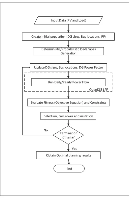
Figure 4.1 Algorithm Flow Chart . . . 52
Figure 4.2 Daily load and active power of PV panels profile for the system. . . 53
Figure 4.3 DG unit connected to the IEEE 37 node test system. . . 54
Figure 4.4 Power losses against peak, medium, and low demand. . . 55
Figure 4.5 Voltage profile of 37 node test feeder. . . 57
Figure 4.6 Voltage profile of 123 node test feeder. . . 59
Figure 4.7 Voltage Profile for base case, case 2 with firm DG, and case 3 with variable DG . . . 60
Figure 4.8 Optimal DG bus connections in the IEEE 37 node test system. . . 63
Figure 4.9 Optimum capacity by DG bus location. . . 64
Figure 4.10 Cumulative distribution of the power capacity for each DG unit. . . 64
Figure 4.11 Cumulative voltage deviation for one year . . . 65
Figure 4.12 Energy losses for 24 hours, for base case, Case 2 with firm DG, and case 3 with variable DG . . . 65
XVIII
Figure 5.2 Daily system load and DG power production profiles . . . 77 Figure 5.3 Diagram of the IEEE 13 Node test Feeders and the two DG
connections. . . 79 Figure 5.4 Daily network losses with CVC application and the two
comparison scenarios . . . 80 Figure 5.5 Daily voltage profile at bus 680, from phase A; with the proposed
method and the two scenarios . . . 81 Figure 5.6 OLTC tap movements for 24 hours, with CVC, and the two
scenarios. . . 82 Figure 5.7 Capacitors status for 24 hours with CVC, and the two scenarios. . . 82 Figure 5.8 Transmission and distribution second test system diagram . . . 83 Figure 5.9 Daily network losses with CVC application and the two
comparison scenarios . . . 84 Figure 5.10 Daily voltage profile at bus 10; with the proposed method and the
two scenarios . . . 85 Figure 5.11 Tap operations for 24 hours, with CVC, and the two scenarios . . . 86 Figure 5.12 Tap operations for 24 hours, with CVC, and the two scenarios . . . 86
LIST OF ABREVIATIONS
CABC Chaotic Artificial Bee Colony
CHP Combined Heat and Power.
CCGT Combined-cycle Gas Turbines.
CAPSO Coordinated Aggregation Power Swarm Optimization. CDF Cumulative Distribution Function
CVC Coordinated Voltage Control. CVD Cumulative Voltage Deviation.
DG Distributed Generation.
DER Distribution Energy Resources. ETS École de Technologie Supérieure. EPRI Electric Power Research Institute. GQ-GA General Quantum Genetic Algorithm.
GA Genetic Algorithm.
HSDO Harmony Search Algorithm with Differential Operator. HRSG Heat Recovery Steam Generators.
IEEE Institute of Electrical and Electronics Engineers.
IC Internal Combustion.
IEA International Energy Agency.
XX
MINLP Mixed Integer Non-linear Programming.
IMO Multi-Objective Index.
MOPI Multi-Objective Performance Index.
MO Multi-Objective.
NREL National Renewable Energy Laboratory.
NiCd Nickel Cadmium.
NLP Non-linear Programming.
OLTC On-Load Tap Changer.
PV Photovoltaic.
PEV Plug-in Electric Vehicles.
PD Population Diversity.
PSO Power Swarm Optimization.
SC Shunt Capacitor.
SGA Single Genetic Algorithm.
SHP Small Hydro Power.
VSF Voltage Stability Factor.
LISTE OF SYMBOLS AND UNITS OF MEASUREMENTS
PLi Active Power Losses at the i line [kW]. Vn Voltage at the n node [P.U].
Vnmin Minimum voltage limit [P.U.]. Vnmax Maximum voltage limit [P.U.]. Vre f Reference node voltage 1 [P.U].
PDGi Active power output at i DG unit [kW]. QDGi Reactive power output at i DG unit [kVAR]. PLoss Active power loss [kW].
QLoss Reactive power loss [kVAR].
PFDGi DG unit power factor.
PDGmin Minimum limit for active power curtailment [kW]. PDGmax Maximum limit for active power curtailment [kW]. QminDG Minimum limit for reactive power injection [kVAR]. QmaxDG Maximum limit for reactive power injection [kVAR]. PFDGmax DGs Power factor maximum limit.
PFDGmin DGs Power factor minimum limit. Taph OLTC tap position at time h.
μSR Solar radiation mean.
XXII
μL Load demand mean.
σL Load demand variance.
MW Mega Watt kW Kilo Watt m Meter km Kilometer oC Degree Celsius s Seconds A Amperes
kva Kilo volt ampere
kvar Kilo volt ampere reactive
F Farad Hz Hertz H Hour min Minute V Volts Ω Ohm CO2 Carbon Dioxide N2O Nitrous Oxide SO2 Sulfur Dioxide
INTRODUCTION
0.1. Background
The electric power system has been for many decades an efficient way to transmit power, from large and centralized production plants, to the homes and industries. The saturation of the network due the continuously growing demand, the concerns about the environmental impact of large electric power plants, changes in the consumer behavior, and the new technologies to harvest energy from renewable resources have change the traditional power production and transmission paradigm. Now, it is feasible to connect small generators to the feeders in a dis-tribution system. In the literature, this connections are called Distributed generation (DG). In traditional power systems, the power flows unidirectional from the generation plants to the distribution system. DG generates power flows from feeders to substations, producing bidirec-tional power flow as stated by (Viawan, 2008).
The existing electric power system was not designed to operate with bidirectional power flow, or to accommodate generators into the distribution system, which is the most sensitive to losses and failures. DG has to be integrated after an extensive planning to avoid negative impacts in the network like voltage rise and interference with control elements. Generally, the most used method to avoid problems with DG, is to limit the amount of power the small generators can inject to the network, and to locate it near to the most congested load centers, although, these solutions do not exploit all the benefits that DG could bring to the network.
In the case of renewable sources like solar photovoltaic and wind, the intermittent nature of these sources presents an additional challenge to their interaction with the network control and stability. It is important to properly locate and determine the optimal amount of power that DG could inject to the grid, without negatively impact the network and maximizing the penetration of DG.
In distribution networks with DG presence, the distribution management system usually dis-connects the distributed energy equipment in case of network failure as recommended in
2
(Basso and DeBlasio, 2004). Advanced control systems can take advantage of the distributed generators interfaces, and their fast time response for curtailment and reactive power output or absorption can be used as a new control element in the network. Nevertheless, the interaction of DG with traditional control devices as OLTCs could derive in interference and excessive control operations. Control actions of each element in the network have to be coordinated with the DG using centralized or coordinated voltage control methods.
The principal objective of this work is to address two principal factors that are present when DG is connected to the grid: Distributed generation units location, and proper control coordination with the system. Thus, a method to determine the optimal location and size of renewables DGs in an unbalanced network is presented. Additionally, this objective is complemented with a coordinated voltage control method to actively manage various renewables DGs units that will participate in the control process.
0.2. Methodology
The two principal objectives, allocation and voltage control, were addressed designing two multi-objective (MO) problems. These MO problems contain the individual objectives: active and reactive power losses, voltage stability, number of control operations, etc. Due the fact that the problems present a non linear behavior and are not concave, the solution method chosen was a genetic algorithm (GA) technique to find the global solution in an efficient way. The methods were tested using the IEEE-node test networks, wich are radial and unbalanced. Software OpenDSS (EPRI, 2015) was used to solve the power flow problem for the unbalanced networks.
0.3. Outline of the thesis
This thesis contains 5 chapters. Chapter 1 gives a literature review about the methods to the DGs allocation and the methods to perform coordinated voltage control with DG presence. Chapter 2 presents the software tools used in this thesis. An explanation of the principal fea-tures of OpenDSS software and a co-simulation example between OpenDSS (EPRI, 2014) and Matlab (MathWorks, 2014), are given. Chapter 3 gives an overview of the main distributed
3
generation energy resources. Chapter 4 proposes a method to optimally locate and size DG connections to an unbalanced distribution system. Chapter 5 proposes a method to determine the optimal settings of control elements, and outputs of DG plants in a coordinated voltage control scheme. Chapter 6 presents the conclusions of this work.
CHAPTER 1
LITERATURE REVIEW
1.1 Introduction
Distributed Generation (DG) is a new term that could refers, depending on the region of the world to: Decentralized Generation, Dispersed Generation, or Embedded Generation. The definition could be divided into different aspects as DG Location and Rating. The International Energy Agency (IEA, 2002) and (Ackermann et al., 2001) agree that Distributed generation is an electric power generation unit that is located and connected to the distribution side of the network. While the Electric Power Research Institute (EPRI) adopts a definition for Distributed Energy Resources (DER), as smaller power sources that can be aggregated to provide power necessary to meet regular demand (EPRI, 2015). DG also can be defined or categorized based on their rating. As suggested by (Ackermann et al., 2001):
Micro distributed generation: <5 kW; Small distributed generation: 5 kW-MW; Medium distributed generation: 5 MW-50MW; Large distributed generation: >50MW;
According to (Koeppel, 2003), plants that exceed 300MW are not considered as DG.
Distributed generation includes a large group of energy sources and technologies. According to the type of resource can be classified into renewables and non-renewables. The most common source of renewable energy is photovoltaic and wind generators, which at the same time, are not dispatchable sources. The non-renewable energy sources more known small combustion engines powered with oil fuel.
6
Depending on the type of source, the technology of the generator and the interface with the grid can vary. For example, synchronous generators are used in combustion generators, or geothermal. While induction and permanent magnet generators are used with wind power, and hydropower. On the other hand, power electronic interfaces are of common use in photovoltaic and fuel cells. Nevertheless, generators and power electronics interfaces can be combined, as in the case of some wind power interfaces that use AC/DC/AC or AC/DC power converters.
1.2 Impacts of Distributed Generation on distribution networks
Distributed generators installations help to reduce some environmental impacts, that cause the traditional electric power system model expansion. DGs have generally fewer cost of instal-lation. Transmission lines are no longer necessary, when DG units are located near the load demand. The environmental benefits are larger when renewable resources are used, generating economical benefits and ensuring the energy provisioning to the local region. Besides the eco-nomical and environmental benefits, DG can generate some impacts that should be considered. Traditional distribution systems were conceived to manage an unidirectional power flow, were the energy flows from the substations to the consumers. The connection of various DG units along the radial system provokes bi-directional or multi-directional power flows. Therefore, the effectiveness of protection equipments as reclosers, breakers and fuses may be degraded, due the change of direction of power flow and the current fault levels (Balamurugan et al., 2012).
The losses on a distribution network depend principally of two factors, resistance of the con-ductors and the current magnitude. To reduce the resistance in the concon-ductors is necessary to invest in network upgrades (new equipment and modern conductors). The second factor has to do with current reduction. It has been demonstrated that the correct capacity planning and connection of DGs near the loads, can reduce the current level in the conductors, reducing the power losses. On the other hand, if the DG capacity is much higher than the load demand, the
7
power losses tend to increase (Méndez Quezada et al., 2006). DG renewable sources are less effective in power loss reduction, due their intermittent behavior (Singhal and Ajjarapu, 2015). The location and capacity of the DG also affect the voltage level in the distribution network. In a normal radial network, the voltage gradually decreases downstream to the loads. In contrast, DG presence cause a change in power flow direction. Reverse power causes voltage rise in the point of connection and near regions. If the DG capacity is high enough, a voltage limit violation could occur. In the same way, OLTCs and SVRs elements mechanism and sensors are not designed to bi-directional power flow. Thus, their operations can be interfered, causing unpredictable behavior in voltage level, deriving in voltage instability, (Abri, 2012).
1.3 Literature Review on Distributed Generation Allocation
Power losses in distribution and transmission networks occur when the current flow through electric lines, transformers and other electric equipments that present electric resistance. Con-sequently, there are two ways to reduce the power losses: Reduce the current through the power conductors or reducing the resistance of the conductors, the second requires increasing the quality of the conductor design, investing in conductors with better materials with mini-mum resistance. On the other hand, reducing the current requires to reduce the load in each feeders, by reducing the electric demand from the consumers.
Besides the traditional methods to reduce power losses, (Hoff and Shugar, 1995) demonstrate that power generators installed along the distribution feeders have the effect to reduce load losses. This is a result of supplying power to the load centers locally, reducing the current level in the distribution lines. Thus, DG location has a directly influence on power losses. In addi-tion, the size of the DG has a direct relationship with the loss reduction or rise, depending of the specific network characteristics, load distribution, and the type of DG, (Ochoa and Harrison, 2011).
Optimum allocation refers to the study of the optimum location of DG connection and the optimum production level, without deteriorate the stability of the system.
8
Several studies have been addressed to find the optimum place and size of distributed generators in the network, either to reduce power losses or to improve voltage stability and regulation. (Teng et al., 2002) proposed a strategy to select the best DG type and the optimal place and size. The authors solve the problem using the value-based planning method, balancing the cost of DG installation and benefits, which include power loss and cost reduction, and improve of reliability. (Haesen et al., 2005) describes a method to optimal placement and sizing of DG with the objective of power losses minimization. The method maintains the voltage profile within the nominal levels. The authors used the genetic algorithm (GA) to find the solution of the non-convex problem. (Kashem et al., 2006) presents a technique to find the optimal operating point of DG and their location and size, using sensitivity analysis in function of power losses and voltage drop. (Ochoa et al., 2006) presents a multi-objective performance index (IMO) to evaluate a distribution network with distribution generation presence. The IMO is used to analyze the impacts on power losses considering different power factor, location and DG size. (Celli et al., 2006) proposed an evolutionary multi-objective method to find the optimal place and size of large amount of DG. The genetic algorithm is used to solve the MO problem. The objectives are the minimization of the capital, operational and energy losses costs, while maximizing the DG penetration. (Singh et al., 2009) used the genetic algorithm optimization technique to find the best solutions for the multi-objective MO problem. The MO problem was based in performance indexes and used different load models. (El-Zonkoly, 2011) presented a multi-objective index based method to determine the size and DG location in a distribution network with no unity power factor and various types of load. The MO problem are composed, in order of importance, of the active power and reactive losses index, the current capacity index, voltage profile index and short circuit index.. The MO problem is solved using a particle swarm optimization (PSO) technique.
(Akorede et al., 2011) stated that the improper DG allocation leads to power losses increment in distribution networks. Thus, the study proposed a single multi-objective. The problem is solved using genetic algorithm technique. A fuzzy control is used to manage the population diversity (PD). The study concludes that this technique is more robust than the single genetic
9
algorithm (SGA) methods. (Moradi and Abedini, 2012) presented an optimization method to locate and size DG using a combination of GA and PSO, with the objective to minimize power losses, and to improve voltage regulation and stability. (Al Abri et al., 2013) proposed a voltage index method to place and size high penetration DG in a distribution network. The optimiza-tion problem is solved using mixed-integer nonlinear programming. The principal objective is to improve the voltage stability margin. This method is able to include the probabilistic nature of renewable DGs, like PV and wind generators. (Kayal and Chanda, 2013) used a new multi-objective PSO method to optimally locate arrays of wind turbine generation and photovoltaic units in a distribution system. A new index called voltage stability factor (VSF), is proposed as an efficient way to evaluate the impact of DG connection. The study concludes that DGs with lagging power factor offers more benefits to voltage profile in distribution lines. (Shaaban et al., 2013) used a GA to find the optimal sizes and locations of DG. The objective functions considered in this work are the cost of system upgrade, energy loss, and costs of interruptions. Also, a variable load-generation model is taken into account to evaluate the method. (Kansal et al., 2013) presents an optimal placement method for different types of DG. The authors use the PSO technique to solve the problem which includes the optimum size also. (Zhao et al., 2014) solved the problem of the optimal location and capacity of DG in a distribution network, taking into account vulnerable nodes. Once the vulnerable nodes are identified, a genetic algo-rithm technique is used to solve the optimization problem. (Zeinalzadeh et al., 2015) proposed a multi-objective problem to locate and size multiple DG and shunt capacitors in a distribution network. The MO problem is solved using PSO and Pareto optimal. The loads are modeled using fuzzy data theory. A method to find the optimum place and size for DG in a distribution network is proposed in (Kollu R., 2015). The method use harmony search algorithm with dif-ferential operator (HSDO) to solve the problem. The objective was to minimize active power losses and to improve the voltage profile. (Mohandas et al., 2015) solved a multiobjective per-formance index (MOPI) problem for DG location and size using Chaotic Artificial Bee Colony (CABC) algorithm. The problem formulation includes active power loss, reactive power loss, voltage profile, and line flow limit index. (Gampa and Das, 2015) developed a multiobjective technique based on a genetic algorithm (GA) to optimal sizing of DG units. The sizing method
10
considers power loss reduction, line load reduction and voltage profile improvement. Also, investment costs included in the optimization problem. The location issue is solved separately using sensitivity analysis. The number of DG units to be allocated are not considered in the op-timization problem. (Ganguly and Samajpati, 2015) presented a DG allocation technique that can work with uncertain variability of load and generation using triangular fuzzy number. The optimization problem is solved using the genetic algorithm. The objectives are to minimize the active power losses and the node voltage deviation.
1.4 Literature review on Coordinated Voltage control methods with Distributed Gener-ation
Voltage regulation in a distribution system consists in keeping line voltages within the nominal limits. The traditional networks have regulations on the equipments that act locally to control the voltage levels. The most common equipments are on-load tap changer (OLTC) and shunt capacitors (SC). Their functioning is based on the premise that power flow is unidirectional, and can be regulated changing the turn ratio in transformers, or by the reactive power control that is directly related with voltage drop.
The connection of DG along the feeders in the distribution system changes the traditional model in which the power flows in one direction only, decreasing, from the substation transformer, to the feeders and the loads. This is due to the power generated in the DG units, that increases the voltage at the connection points. Thus, DG can interfere in the normal performance of voltage and reactive power regulation. Therefore, it is necessary to properly coordinate the DG units with the OLTC and shunt capacitors to avoid damaging the voltage profile and to not worsen the power losses.
In this section a literature review of various coordinated voltage control methods is presented. (O’Gorman and Redfern, 2008) stated that the common practice is to avoid DG to act in the voltage control. Thus, authors proposed a method to control the voltage locally, at the point of common coupling (PCC) between the DG and the grid. Sansawatt et al. (2010) proposed a DG
11
decentralized control method for DGs. Using power factor and voltage control modes to keep the voltage levels at the connection bus between the limits. Also includes DG production cur-tailment capability in case of voltage rise. Local control methods allow to reduce the operation costs of DG and do not need communication channels to operate.
Another approach is to use the DG as an active control element in the distribution networks. DG as control element could offer many advantages due to their fast response to change their active and reactive power output. As proposed by (Dai et al., 2004) and (Kim et al., 2015). However, the control actions of the DGs, if are not coordinated, could interfere with the control actions of regulation equipment such as OLTCs, static var compensators, and SCs.
Borghetti et al. (2010) proposed the improvement of the Distribution Management Systems (DMS) from an active distribution network approach. When DG reaches important penetration levels, the network can take all the advantages of DGs: as an active and reactive power source and as a fast voltage control element. Additionally, the rest of the network resources could be coordinated with DG actions.
(Richardot and Viciu, 2006) proposed that distributed generation could act as an actively el-ement in the coordinated voltage control (CVC) in a distribution network system. They pro-posed to apply the same control principles of transmission on the distribution network. The CVC aims to coordinate all the networks resources present at certain time, in order to optimize and to improve the power delivery and the quality of energy. Similar approaches have been proposed in various works. Tsikalakis et al. (2008) study the CVC approach to operate on line and off line microgrids with several types of DGs.
The optimization and coordination of several networks elements comprehends a combination of continuous (DG power output) and discrete variables (OLTCs and SCs control actions). Thus, the optimization problem becomes more and more complex. In this context, multi-objective solving techniques have been proposed.
12
(Viawan and Karlsson, 2008) presented an optimization method for CVC and reactive power control with and without DG. Authors conclude that the involvement of DG in the voltage control contributes in the reduction of losses and diminish the number of OLTC operations. Capitanescu et al. (2014) study a centralized optimization method to minimize the power cur-tailment of DG, taking into account traditional voltage control elements (OTLCs, SCs, and Remotely controlled switches) and DG operation modes. (Paaso, 2014), use a CVC approach in a multi-objective problem to minimize the power losses and maximize the power extracted from intermittent resources as PV.
Evolutionary algorithms are vastly used to solve this type of problems. The following works, use similar optimization problems using two of the most popular algorithms: Particle Swarm Optimization (PSO) and the genetic algorithm (GA). (Sarmin et al., 2013) present a voltage and reactive power control strategy, using a mixed-integer nonlinear programming problem. The authors solve the problem using PSO. The optimization problem incorporates forecast data for the load and generation 24 hours ahead. (Vlachogiannis and Lee, 2006) uses a similar optimization problem approach. But, the problem is solved using a new particle swarm op-timization algorithm called Coordinated Aggregation (CAPSO). (Kim et al., 2015) presents a method to control the voltage in distribution networks, using DG as ancillary service to provide reactive power. The optimization method includes shunt capacitors and OLTCs in coordina-tion with DG dispatch. The problem is solved using PSO. (Su et al., 2011) use a binary PSO to solve the optimization problem. The method includes a coordinated network reconfiguration and volt/var control to limit the DG power injection at the connection point. Both, the load and generation are modeled as variable in time. (Senjyu et al., 2008) proposed an optimal voltage control for distribution networks, using DG with OLTCs, shunt capacitors and voltage regula-tors to maintain an stable voltage level at feeders and to reduce the power losses. The genetic algorithm is used to solve the optimization problem. (Vlachogiannis and Østergaard, 2009) solved the optimization problem for a coordinated voltage control using the general quantum genetic algorithm GQ-GA. The method finds the optimal settings for various control elements in a distribution network including DG.
13
(Shivarudraswamy and Gaonkar, 2012) presents a method to determine the optimal set points of the control elements in a distribution network, including DG. The problem formulation use power losses reduction and voltage regulation. Additionally, the load and generation pro-file are considered time-varying. The problem is solved using the genetic algorithm technique. (Abapour et al., 2014) proposed a multi-objective problem that minimize costs of active and re-active poser losses, by the coordination of control elements including DG. The proposed prob-lem is solved using Non-dominated Sorting Genetic Algorithm. In (Azzouz and El-Saadany, 2014), authors developed a voltage regulation method that obtains the optimal settings for OLTCs and DG reactive power. Additionally, a new hysteresis controller for the OLTC is pre-sented. The objective is to achieve proper voltage regulation and to reduce the number of tap operations.
CHAPTER 2
DISTRIBUTION NETWORK MODELING WITH OPENDSS
This chapter describes the software used to simulate the distribution networks used in this thesis. The methods described later in this work, needs to be tested on unbalanced radial distribution networks. Therefore, OpenDSS was used to obtain the power flow solutions, and MATLAB was used to run the optimization algorithms.
The traditional electric distribution network has resisted decades without mayor improvements or changes. Distribution networks were designed under the premise that customers, only could be passive consumers. Nevertheless, awareness about the environmental and economics ben-efits of energy efficiency and distribution generation, have been changing the way companies and consumers consider the distribution network. Modern distribution networks are including distribution generation, new control systems, active demand, etc.
The traditional modeling of distribution networks work with balanced networks, and unidirec-tional power flows. For tradiunidirec-tional systems, simulations under this constraints, give a very good approximation of the steady state of the network. On the other hand, the modern distribution systems requires simulation tools that allows to work with bidirectional power flows, distribu-tion generadistribu-tion models, unbalanced networks, time varying demand and generadistribu-tion profiles, etc.
OpenDSS is a distribution system simulator that fits with the new challenges of distribution systems.
2.1 OpenDSS
In this section, OpenDSS software is described, most of the content of this section is based on its reference guide by (Dugan, 2012).
16
OpenDSS is a distribution system simulator. DSS means Distribution System Simulator. It is an open source software supported by the Electric Power Research Institute (EPRI). The basic implementation is an executable program script-based, and numerical and graphical solutions. The second possible implementation is a COM server DLL which can be used from third platforms as Matlab, Excel VBA, Python, etc. This feature permits to increase the variety of uses and applications that OpenDSS could perform. The software supports rms steady-state analysis. Although the software was originally intended to simulate distributed generation. OpenDSS can simulate more complex features like harmonics analysis, energy efficiency and smart grids applications.
The principal applications are:
• Distribution Planning and Analysis. • General Multi-phase AC Circuit Analysis.
• Analysis of Distributed Generation Interconnections. • Annual Load and Generation Simulations.
• Risk-based Distribution Planning Studies. • Probabilistic Planning Studies.
• Solar PV System Simulation. • Wind Plant Simulations. • EV Impacts Simulations.
• Development of IEEE Test feeder cases
Some of the solution modes implemented in OpenDSS are:
• Snapshot mode: Which is a direct power flow execution that reflects the actual steady state of the network.
17
• Daily mode: This mode performs power flow and control solutions for each time increment. 1 hour increment for 24 hours for default.
• Yearly mode: Performs solving actions for 8760 hours, the time period can be changed from 1 hour to any interval.
• Dutycycle mode: Small time increments in seconds. • Harmonics.
• Dynamics transients.
• Fault study and Monte Carlo fault study.
The COM interface permits to increment the number solution types, which can be adapted according to the necessity of the researcher or user. OpenDSS can execute this solutions in radial distribution networks models and meshed distribution systems, where the circuit model can be multi-phase and unbalaced.
There are two posible power flow solutions: iterative and direct. By default, the iterative solution is performed each time. The Iterative solution considers loads and DG as injection sources. While the Direct solution take loads and generators as admittances, to be solved without iterations.
Fault studies also can be performed in OpenDSS. In three ways: A conventional fault study for all phases and circuit elements. The snapshot fault, where the user could place specific type of faults and locations. And Monte Carlo fault study, the user select specific elements and locations, and the program randomly chooses one fault at a time.
It is also possible to perform harmonic analysis, due the fact that OpenDSS is actually a fre-quency domain circuit solver. After doing a power flow solution, then, the harmonic solution is executed for each frequency the user sets. Loads, generators, voltage and current sources participate in the harmonic solution. Additionally, PV system model and Storage model could be considered for harmonic solution.
18
The Dynamic solution mode allows to simulate electromechanical transients of generators. The generator dynamic model is a single-mass model. To more sophisticated generators models, the user has to create a new DLL generator model, or to use a third party program to control the generator.
2.2 Simulation of a Medium Voltage Network with OpenDSS.
A brief introduction to the basic commands for the script interface of OpenDSS is presented. Then an example of an unbalanced 13-node distribution network with time varying load and a PV distributed generator is exposed in this section.
The stand-alone installation of OpenDSS permits to enter the functions and commands in text format, in any order. The compiler organizes the scripts of each circuit element and creates the components and the complete system.
2.2.1 New Circuit
To create a new circuit, it is necessary to determine the base frequency. the command: "Set defaultbasefrequency=60" should be used to do this action.
It is important to set the voltage source for the circuit, which should be considered the reference bus, necessary to initiate the power flow. It can be defined through a line or a transformer. The command that defines the voltage source should have this format:
New circuit.ExampleName basekv=115 pu=1.00 angle=0 Bus1=SourceBus R1 = Value X1 = Value R0=Value X0=Value phases=3.
Where "Bus" is the bus connected to the source. "basekv=" is the line to line voltage in KV. With "pu=" the voltage level at the source can be set in p.u. units. "Angle=" determines the phase base angle in degrees. Also, it is possible to set the positive and zero sequence of the resistance and reactance of the source with "R1=,R0=,X1=,X0=" respectively.
19
2.2.2 Transformer
The substation transformer can be defined using:
"New Transformer.ExampleTrans phases=3 windings=2 wdg=1 bus=SourceBus wdg2 = 2 bus = Bus.Name conns=(delta,wye) kvs=(115,4.6) kvas=(5000,5000) xhl=(8 1000 /) %loadloss=0" The user specifies the number of phases, and the number of the windings. With "kvs=" and "kvas=", the base rated voltage and KVA of each winding is set. "xhl=" allows to set the high winding to low winding reactance. And the percent of losses in the transformer is represented with "%loadloss=".
A regulator transformer could be included following this format:
"new regcontrol.RegExample transformer=ExampleTrans winding=2 vreg=122 band=2 ptra-tio=20 ctprim=700 R=3 X=9".
"Ptratio=" specifies the ratio of the Potential Transformer that converts the controlled wind-ing voltage to the regulator voltage, the default value is 60. "band=" is the bandwith of the controlled bus in volts. "CTprim=" defines the rating of the primary CT for the line current to control current, in Amperes. "R=" and "X=" set the value of the line drop compensator in Volts.
2.2.3 Lines
To define the lines of a distribution system, we should first set the "linecode", which speci-fies the line admittance matrix. Various lines can use the same "linecode". Nevertheless the admittance values can be written directly in the "line" command script.
"New linecode.codeExample nphases=3 R1=1.3292 X1=1.3475 units=km".
"New Line.lineExample Phases=3 Bus1=Bus1.name Bus2=Bus2.name LineCode = codeEx-ample Length= 0.25 units= km"
20
To define the line, it is necessary to establish the two connection buses, the "length" of the line, the longitude unit and the number of phases.
The linecode with a larger admittance matrix could be written as follows:
"New linecode.lineExample nphases=3 rmatrix = (0.3465 | 0.1560 0.3375 | 0.1580 0.1535 0.3414 ) xmatrix = (1.0179 | 0.5017 1.0478 | 0.4236 0.3849 1.0348 ) units=km"
2.2.4 Loads
The load element is defined through its nominal active and reactive value "kW" and "kvar" respectively. Additionally, the load script accepts various properties as follows:
"new load.loadExamplebus1=B phases=3 Conn=Wye kV=33 kW=5000 kvar=1640 model=1 model=1"
When the reactive value of the load is not defined, the power factor should be set with "pf=". There are different load models available in the program:
• Model 1: constant P and Q.
• Model 2: Constant impedance load. • Model 3: Constant P and quadratic Q. • Model 4: Linear P and Quadratic Q. • Model 5: Constant P and constant current. • Model 6: Constant P; and Q fixed nominal value.
• Model 7: Constant P; and Q is fixed impedance at nominal value. • Model 8: ZIP model.
21
Load variability can also be included in the command: "Daily=", "yearly=" or "Growth=" are used to call the load shapes that will determine the load behavior on daily, yearly or duty simulation modes.
2.2.5 Control Modes
The default control mode in OpenDSS is "Static". The sentence "set controlmode=OFF", turns off all control actions.
In mode static, time is not considered, and the control actions are executed for each power flow solution. This mode is the standard for snapshot, daily and yearly mode.
Modes Time and Event realize control actions driven by a time or a event, respectively.
2.2.6 Solution Modes
With the command "Mode=" the type of solution for the active circuit can be set. There are various solution modes. To solve the circuit for a specific configuration without time variation modes Snapshot and Direct could be used. The mode Snapshot is preferred when loads need to be modified.
Modes Daily, Yearly and Dutycycle, perform a series of solutions following a time load profile or an specific increment as in the case of Dutycycle.
2.2.7 Monitors and Meters
The Monitor object is a power monitor that is connected to any terminal of the circuit. Records the variables of voltage, current and power of all phases. The monitor exports the data in a CSV file.
The code has the following format:
22
With "Element=" as the circuit element where the monitor is connected. "Terminal=" is the ter-minal of the circuit element, could be defined as 1 or 2. Monitor can observe various variables depending of the configured "Mode=". "0" is the standard mode that records, Voltage, Current, and complex values. "1" records the power of each phase. "2" the Tap changes of a regulator. "3" records the state variables.
The EnergyMeter object is an energy meter which can be connected to any circuit element. Registers the exports and imports of energy, consequently, losses and overload values. Not only at its point of connection, but at a defined region in the circuit.
The command can be written as:
"new energymeter.ExampNetwrk element=transformer.TranExample terminal=1"
The Monitor and EnergyMeter can export data after the solution command "solve". The commands "monitor.MonExample.action=take" and "energymeter.ExampNetwrk.action=take" should be written in order to record all the values. After, the commands "export monitor Mon-Example" and "export meters" are used to export the data to the CSV files.
2.2.8 Simulation of a 13-node distribution network.
The Distribution Test Feeder Working Group, affiliated to the IEEE Power and Energy Society, published various test-feeder models. These test-feeders are used by researchers to evaluate and test unbalanced three-phase radial system new algorithms (PES, 2013). One of these test-feeder cases is the 13-bus Feeder, used in this thesis.
The IEEE 13-node test feeder is a small three phase unbalanced distribution system. It has short and high loaded, it has only one substation with three phase voltage regulator. Overhead and underground lines (Kersting, 1991). The one line diagram is shown in Fig. 5.3.
First the circuit is declared: "new circuit.IEEE13Nodeckt basekv=115 pu=1.0001 phases=3 bus1=SourceBus Angle=30 MVAsc3=20000 MVASC1=21000"
23
The substation transformer code is: New Transformer.Sub Phases=3 Windings=2 XHL=(8 1000 /) wdg=1 bus=SourceBus conn=delta kv=115 kva=5000 %r=(.5 1000 /) XHT=4 wdg=2 bus=650 conn=wye kv=4.16 kva=5000 %r=(.5 1000 /) XLT=4
Note that values can be written in polish notation.
Voltage regulators have the following code, for one phase:
New Transformer.Reg1 phases=1 XHL=0.01 kVAs= [1666 1666] Buses= [650.1 RG60.1] kVs= [2.4 2.4] %LoadLoss= 0.01 new regcontrol.Reg1 transformer= Reg1 winding= 2 vreg= 122 band= 2 ptratio= 20 ctprim= 700 R= 3 X= 9.
Lines and loads can be defined as follows.
"New Load.671 Bus1= 671.1.2.3 Phases= 3 Conn= Delta Model= 1 kV= 4.16 kW= 1155 kvar= 660". "New Load.634a Bus1=634.1 Phases=1 Conn=Wye Model=1 kV=0.277 kW=160 kvar=110".
"New Line.650632 Phases= 3 Bus1= RG60.1.2.3 Bus2= 632.1.2.3 LineCode=mtx601 Length= 2000 units=ft" "New Line.632670 Phases= 3 Bus1= 632.1.2.3 Bus2= 670.1.2.3 LineCode= mtx601 Length= 667 units= ft"
The 13-node test system have many more elements, the complete code and circuit definitions are in Appendix 1. The script interface looks like in Fig. 2.1
After solving the circuit it is possible to show some results, with the command "Show". For example:
• "Show Voltages LN Nodes" • "Show Losses"
24
Figure 2.1 OpenDSS script interface
Which results in pop-up notepad windows, as shows the Fig: 2.2
Figure 2.2 Node voltage, circuit losses and taps movements presented in text interface
The script interface also has the feature that allows to show graphics results. With the command "plot profile phases=all", a graphic showing the voltage profile is obtained. Fig. 2.3
25
Figure 2.3 Voltage profile for the 13-node test system
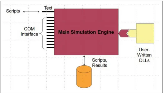
2.3 Co-simulation OpenDSS with Matlab
In this section, a distributed generator is connected to the 13-node test system. Also, a load profile to vary the load level during the day, and a production profile to emulate the intermittent behavior of the PV panels is incorporated, using MATLAB as the programming interface. Through MATLAB, scripts and commands can be entered to the main simulation engine of OpenDSS. In the same way, OpenDSS simulation engine can export results and scripts to MATLAB through the COM interface. In the Fig. 2.4 (Dugan, 2012) the OpenDSS structure can be appreciated.
26
Figure 2.4 OpenDSS structure
2.4 OpenDSS-MATLAB initiation
From a new MATLAB .m file, the commands used to initiate the COM interface are: "[DSSStartOK, DSSObj, DSSText] = DSSStartup;"
In the example presented here, the main simulation engine will solve the power flow of the 13-bus system, as in the last section. The PV system, load profile, daily simulation, and control schemes, will be commanded from MATLAB interface and sent to the OpenDSS core. Both, .dss file and the .m file should be placed in the same file path.
On the editor window in MATLAB, the script which calls the file circuit from OpenDSS is:
1 if DSSStartOK
2 DSSText.command='Compile (C:IEEE13Nodeckt.dss)'; 3 DSSCircuit=DSSObj.ActiveCircuit;
27
2.4.1 Load Shapes
The load shapes, for the load demand and the production curves, are important to perform the sequential power flow solutions. In this example, the interval between values is 1hr for 24hrs, 24 values in total.
The matrix of values can be entered in the line command, or be called from a .csv file. In the command line the number of points is defined with "Npts=". Those values are multiplied with the base kW values of loads or DG capacity.
Let the loadshape be called: daily. And the production curve: MyIrrad, which correspond to the irradiation values of the PV panels. These values are represented in chapter 5, Fig.5.2
1 DSSText.Command = 'New loadshape.daily npts=24 interval=1
2 mult=(0.3 0.3 0.3 0.35 0.36 0.39 0.41 0.48 0.52 0.59 0.62 0.74... 3 0.87 0.91 0.94 0.94 1.0 0.98 0.94 0.92 0.61 0.60 0.51 0.44)'; 4 DSSText.Command = 'New Loadshape.MyIrrad npts=24 interval=1 5 mult=[0 0 0 0 0 0 .1 .2 .3 .5 .8 .9 1.0 1.0 .99 .9 .7 .4 .1... 6 0 0 0 0 0]';
In the same way the solution mode and the control mode should be written:
1 DSSText.Command = 'set mode=daily';
2 DSSText.Command = 'Set controlmode=static';
2.4.2 Photovoltaic system simulation
A very useful feature in OpenDSS is the PVsystem Element Model, developed by the (EPRI, 2011). The last version of the DLL model, implements a PV array model and the PV inverter. For its use, it is necessary to declare the "XYcurves". The points in the commands describe
28
how the active power max power point Pmppvaries with the rated temperature at kW/m2. The
other array represents the efficiency curve fro the inverter.
1 DSSText.Command ='New XYCurve.vv_curve npts=4 Yarray= 2 (1.0,1.0,−1.0,−1.0) XArray=(0.5,0.95,1.05,1.5)';
Then, the internal state variable has to be setup. The "irradiance=" sets the net irradiance after the load shape application. The "panelkW=" is the net power in kW, in function of the irradiance and the temperature. Alternatively, "kVA" and "pf=", apparent power and power factor. For more detailed description, PVSystem Object manual is available in the installation folder of OpenDSS.
1 DSSText.Command ='new PVSystem.plant4a phases=3 bus1=680 2 kV=4.157 kVA=1500 irradiance=1 Pmpp=1728 pf=1 daily=MyIrrad';
2.4.2.1 Inverter Control
The inverter control object in OpenDSS is named InvControl. Basically, this element, control the PVSystem Object, in three possible ways:
• Intelligent Volt-Var Function. • Volt-Watt Function.
• Dinamic Reactive Current Function.
In this example, the Volt-Var function is used. In this function, the inverter controls the vars response based on the voltage at the point of connection, and the available KVA at determined time. The command permits to enter a vector of number that describes the volt-var curve, where the user can configure a dead-band or a hysteresis interval, (Smith, 2013).
29
The command to be entered in matlab is as follows:
1 DSSText.Command ='New InvControl.InvPVCtrlb mode=VOLTVAR 2 voltage_curvex_ref=rated vvc_curve1=vv_curve EventLog=yes';
Fig.2.5 shows the code in the matlab editor. For this example two PV plants, with a capacity of 1.5MW are connected to the nodes 680 and 671 respectively. The total capacity of the PV plants equals the total power of the 13-node test system. The complete code can be found in the Appendix 2 of this thesis.
Figure 2.5 OpenDSS code in MATLAB editor
2.4.3 Simulation and results
From Matlab, all data generated from OpenDSS can be used. Any type of graphics can also be performed.
For example, voltage from the three phases of node 680 can be graphic to see the impact of the PV plant, at the point of connection.
30
In Matlab, command "DSSCircuit.ActiveBus.puVoltages; " and "DSSCircuit.losses" are used to extract voltage values and losses from the circuit. These commands are written after the "DSSCircuit.SetActiveBus(’680’)" in order to consider only the bus 680.
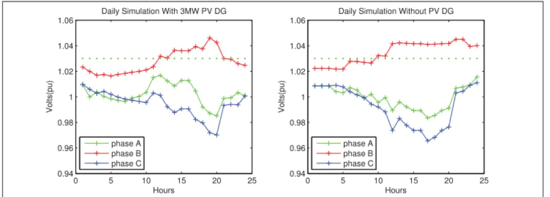
By creating an iterative loop for 24 solutions, Fig. 2.6 is obtained. Where it can be observed a comparison for the voltage levels variation, within 24 hours, before and after the PV connection at bus 680. 0 5 10 15 20 25 0.94 0.96 0.98 1 1.02 1.04 1.06
Daily Simulation With 3MW PV DG
Volts(pu) Hours phase A phase B phase C 0 5 10 15 20 25 0.94 0.96 0.98 1 1.02 1.04 1.06
Daily Simulation Without PV DG
Volts(pu)
Hours phase A phase B phase C
Figure 2.6 24 hour voltage variation at point of connection bus 680
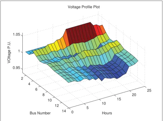
As an example, of the COM interface utility a 3D graphic showing the voltage profile of all 13 nodes variation during 24 hours was generated as shown in Fig. 2.7.
31 2 4 6 8 10 12 14 0 5 10 15 20 25 0.95 1 1.05 Hours Voltage Profile Plot
Bus Number
VOltage P.U.
CHAPTER 3
DISTRIBUTED GENERATION TECHNOLOGIES
3.1 Introduction
This chapter presents a revision of various distributed generation technologies, and the prin-cipal challenges with their connection to the distribution network. The concept of distributed generation is scattered, but generally refers to small scale generation as stated in the intro-duction of this thesis. Units categorized as distributed generation consist in a compendium of several technologies including traditional generators (Combustion Engines) and non-traditional generators (Fuel cells, Storage devices, Renewables), (El-Khattam and Salama, 2004). In the same manner, traditional generators can be named as dispatchable and renewables sources as non-dispatchable due to their intermittent nature. The best examples are Photovoltaic and wind generators. Distributed generators, depending on the local regulation can be owned by con-sumers, private investors or by the utilities.
Every DG technology presents different challenges depending of the energy source, availabil-ity, capacity and connection to the grid. However, the proper addressing of these issues gener-ates technical and economical benefits.
3.2 Combustion Engines
3.2.1 Internal Combustion Engines
Internal Combustion Engines are one of the most traditional and mature technologies used as distributed generation. Internal combustion engines (ICs) converts the explosion energy cre-ated by the combustion in mechanical energy, which drives the electric generator. The installed capacity of ICs could be from 1kW to 5MW, the capital cost are reduced compared with other technologies. Combustion engines are preferred as backup power systems and distributed gen-eration. This is due to its fast start up and simple control. On the other hand, exist some
34
important challenges with ICs, like: Unpredictable fuel cost, high cost of maintenance, and high contaminant gas emissions CO2, N2O, SO2. (Dean et al., 2011) stated that the price for
KW is around $900 to $3000, and the efficiency is 21.3 to 44 percent. Thus, the convenience of 24/7 use of ICs is at least debatable.
3.2.2 Gas Combustion Turbines
A gas turbine produces mechanical energy, expanding great amount of air from a compres-sion and heated process. An electric generator converts the mechanical energy into electrical energy. The capacity of gas turbines are larger than ICs, from 30kW to 250MW, with an ef-ficiency around 30 to 45 percent. Also, estimated cost per KW is about $2000, (Dean et al., 2011). Although, gas combustion turbines produce less pollutants than ICs, they still produce contaminants as nitrogen oxides and carbon monoxide. (EPA, 1995)
3.2.3 Micro-turbines
A Micro-Turbine (MT) is a small capacity combustion engine with a capacity limited between 25-500 kW. It can be driven by natural gas, hydrogen, propane or diesel. The efficiency is about 20-30 percent with the use of recuperation system, which recuperates the heat from the exhaust system and reincorporates in the air entrance, boosting the air temperature. Also, its characterized by low emission of nitrogen oxides (Capehart, 2014). MTs are a gaining adoption because its reduced size, light weight compared with ICs and reduced maintenance costs due the less number of moving parts, (El-Khattam and Salama, 2004).
3.2.4 Combined Heat and Power
Combined Heat and Power (CHP) is a compendium of system that seeks to use the residual heat from a combustion engine to generate electricity or to use it for heating. CHP increments the overall efficiency of power generation technologies based on gas and fossil fuels. For example, an internal combustion engine increment its efficiency from 44% to 80% using CHP. In the
35
same way, gas turbines with CHP increments their efficiency to 85% (Dean et al., 2011). In theory, any combustion engine produce heat as secondary product that is dissipated into the air. CHP system consists in the same structure of combustion engines, but, includes heat recovery and transfer systems. CHP systems based in gas turbines, incorporates Heat Recovery Steam Generators (HRSG) to high pressure steam generation. The Combined-cycle Gas Turbines (CCGT) increments the efficiency of HRSG systems, which use a steam turbine with a back pressure system as stated by (Lako, 2010).
3.3 Fuel Cells
This distributed generation technology generates energy using chemical reactions. Unlike com-bustion engines, the fuel used in the fuel cell does not burn, thus avoiding the waste of excessive heat. Basically, fuel cells have the structure of a battery, with an anode and a cathode, separate by an electrolytic membrane. Oxygen and hydrogen are pushed through the membrane, the atomic reaction creates free electrons from the hydrogen atom, generating an electric current. The product is a molecule of water and some heat (El-Khattam and Salama, 2004). Fuel cells capacities varies from 1kW to 3MW (Dean et al., 2011).
Fuel cells have the lowest emissions compared with engines technologies and efficiency be-tween 40 and 60 percent. On the other hand, they has the highest capital and maintenance costs, (Dean et al., 2011).
3.4 Storage Devices
These devices that store energy, traditionally used for backup purposes. In distribution gener-ation are used to supply power during high demand periods. And, they can be used to smooth the production curve of intermittent sources as photovoltaic and wind generators. Batteries and flywheels are classified as storage devices (Srivastava et al., 2012).
36
3.4.1 Flywheels
Flywheels are storage device that have a mechanical storage mechanism. The mechanism is a rotating mass that is connected to a motor and to a generator. They take the energy from the motor, store this energy as a kinetic energy. As the kinetic energy is drained, the flywheel rotation velocity decreases, and this energy is converted to electricity for the generator con-nected. The variable output frequency and power are driven for the power electronic interface. Many systems permit to combine the motor and the generator in a single device then reducing its complexity and its size. New materials and power electronics have increased the flywheels input and output capacity, and determine charge cycles as large as 90000 charge-discharge cycles, and have a capacity of about 400 kW (Hebner et al., 2002).
3.4.2 Batteries
Batteries are the most know devices to store energy. This technology is in use for more than a century, it consists in an array of cells containing an anode and a cathode linked by an elec-trolyte compound to facilitate the flow of electrons. Their applications on distributed gener-ation are in backup for PV and wind systems. They are also used to smooth the production curve of DG sources and to improve the energy quality parameters, (Srivastava et al., 2012) and (Carrasco et al., 2006). Future use of batteries at great scale, is the use of Plug-in Electric Vehicles (PEV) connected to the grid to sustain network parameters and supply energy during peak hours (Han et al., 2012).
Batteries can be classified after their depth of discharge, cost, charge cycles, efficiency and maturity of the technology. The technology refers principally to the chemical used, the lead batteries are: Lead acid, Lithium Ion, Sodium Sulphur (Nas), Nickel Cadmium (NiCd) and Zinc Bromide. Lead acid and NiCd are the most mature technologies in batteries, and have an average efficiency between 72-78%, and a lifespan of over 3000 cycles. For DG applications lead acid batteries are preferred due its low cost (Coppez et al., 2010).
37
3.5 Renewables
Power generation with zero emissions is possible using renewable resources as wind, sun, geothermal and hydro power to cite the most popular. Although, there exist multiple techniques to obtain energy from many other sources knowing as energy harvesting, In this section, they will not be taken into account due the reduced energy production and the immaturity state of the technology.
3.5.1 Photovoltaic generators
Photovoltaic (PV) generators are devices that generates electric current from a semiconductor material interacting with light energy. A photon impacts a semiconductor layer moving elec-trons to another cell, creating a current flow. Electricity produced for PV is DC, AC is obtained with the help of inverters connected to the PV arrays (FEMP, 2012).
Solar power is a wide available resource, but the efficiency of PV technology is highly de-pendable of clear sky. Clouds shadow reduces the power output of PV panels. Thus, proper geographic location is a restriction for the use of this technology (El-Khattam and Salama, 2004).
The principal components of PV technology are: PV array, inverters, and in some cases, battery banks. The PV modules is the principal part, it converts solar energy into electricity. Generally, a typical solar panel is manufactured to operate for 25 years. Is the most robust part of the system, and the maintenance cost is very low, compared with other technologies. The inverter converts DC power to AC, used in most applications. Further, modern inverters are capable to synchronize their frequency with the grid, for grid-connected applications. Some PV system includes battery banks to storage energy produced by the panels during sun light hours, and provide energy at night time, (FEMP, 2012).
The principal DG applications are: PV panels roof mounted, where, each home should be connected to the grid, inverters should be frequency synchronized and PV plants to sizes from
38
1 to 10MW. Special planning and operation have to take place in order to obtain the mayor benefits. PV plants could be connected in parallel to the grid, the power interface is responsible to disconnect the system when a fault is detected, (Basso and DeBlasio, 2004). PV plants also can be connected to distribution networks. Besides providing energy, they are being used to control voltage and power, and to reduce losses. (Thomson and Infield, 2007) and (Smith, 2013).
3.5.2 Wind Turbine generators
Wind turbines transform wind power into electric energy. In a complete wind energy conver-sion system (WECS), the turbine converts the wind power to mechanical power, then it is con-verted to electric energy by the electric generator integrated. The atmospheric and geographic factors determines the amount of output power (Zahedi, 2015). Traditionally, the mechanical rotor frequency has the same grid frequency, creating limitations in the amount of power de-livered by the WECS, and quality issues. But, current technologies like variable-speed wind turbines, where rotation frequency is decoupled from the grid, increments the efficiency and expands the applications of wind generation systems on distributed generation.
Variable speed wind generators, includes modern AC-DC-AC converters. Allowing WECS to be connected on electric power distribution systems, and to be used on control applications, because the power electronics interface permits to vary the active and reactive power output faster than traditional control devices (Hunyár and Veszprémi, 2014). Also, the inertia of the rotor could be used in frequency stability support on fault cases (Zhang et al., 2013). Ad-ditionally, the power electronic interface creates a DC link, between the AC converters, this DC link is used to connect the WECS to storage devices (Aktarujjaman et al., 2006). Other power generators like PV can be connected to this DC link, which is named hybrid generation (Wang and Lin, 2007).
Wind turbines have in average 30 years of life expectancy. To large installed generation projects >1.5MW, the cost per kW is between $1,800 and $2,000. This cost increment as the project