Mode Selection in Device-to-Device Communications
by
Maryam HABIBIMAREKANI
THESIS PRESENTED TO ÉCOLE DE TECHNOLOGIE SUPÉRIEURE IN
PARTIAL FULFILLMENT OF THE MASTER DEGREE
M.A.Sc.
MONTREAL, NOVEMBER 1, 2018
ÉCOLE DE TECHNOLOGIE SUPÉRIEURE UNIVERSITÉ DU QUÉBEC
© Copyright reserved
It is forbidden to reproduce, save or share the content of this document either in whole or in parts. The reader who wishes to print or save this document on any media must first get the permission of the author.
BOARD OF EXAMINERS
THIS THESIS HAS BEEN EVALUATED BY THE FOLLOWING BOARD OF EXAMINERS
Mr. Zbigniew Dziong Thesis Supervisor
Department of Electrical Engineering, École de technologie supérieure
Mrs.Christine Tremblay, President of the Board of Examiners
Department of Electrical Engineering, École de technologie supérieure
Mr. Michel Kadoch, Member of the jury
Department of Electrical Engineering, École de technologie supérieure
THIS THESIS WAS PRENSENTED AND DEFENDED
IN THE PRESENCE OF A BOARD OF EXAMINERS AND PUBLIC ON “OCTOBER 4 2018”
ACKNOWLEDGMENT
I would like to express my deep and sincere gratitude to my research supervisor, Prof. Dziong Zbigniew. Prof. Dziong whose expertise, understanding, and patience, added considerably to my graduate experience. I thank him for his untiring support and guidance throughout my journey. Besides my supervisor, I would like to thank Dr. Armin Morattab for his support at various stages of this research project.
This journey would not have been possible without the support of my family and friends. To my family, thank you for encouraging me in all of my pursuits and inspiring me to follow my dreams. I am especially grateful to my sister and my brother-in-law who supported me emotionally and financially. I always knew that you believed in me and wanted the best for me. Thank you for teaching me that my job in life was to learn, to be happy, and to know and understand myself; only then, could I know and understand others.
I would like to give special thanks to my nephew, Yashar. Thank you for making me more loving. Thank you for bringing me the most happiness, I have ever felt, when your little hand is in mine. Thank you for reminding me what a true belly laugh is when one erupts from deep in you. Thank you for teaching me how to be responsible for another’s life. You have become my world, little guy, and the only thing I can say is thank you.
To my friends, thank you for listening, offering me advice, and supporting me through this entire process. Thank you for giving me your time. I believe a person’s most precious gift that can give to anyone is his/her time because you can never take it back and you always give me that. I am deeply thankful for it.
SÉLECTION DE MODE DANS DES COMMUNICATIONS DE DEVICE-TO-DEVICE
Maryam HABIBIMAREKANI
RÈSUMÈ
La communication de Device-to-Device (D2D) fait référence à une technologie permettant aux périphériques de communiquer directement entre eux, sans envoyer de données à la station de base et au réseau principal. Cette technologie a le potentiel d'améliorer les performances du système, d'améliorer l'expérience utilisateur, d'augmenter l'efficacité spectrale, de réduire la puissance d'émission du terminal, de réduire la charge du réseau cellulaire et d'étendre les applications cellulaires.
Dans les communications D2D, les UEs peuvent sélectionner parmi différents modes de transmission (TM) définis en fonction du partage de ressources de fréquence à savoir le mode privilégié, «reuse mode» et mode cellulaire. En mode privilégié, la communication D2D est directe et les données sont transmises via la liaison D2D par les ressources de fréquences orthogonales aux utilisateurs cellulaires afin qu'il n'y ait aucune interférence. En «reuse mode», les données sont transmises via la liaison D2D en réutilisant les mêmes ressources de fréquence qui sont utilisées pour un utilisateur cellulaire. Ce mode provoque des interférences sur les récepteurs, toutefois, l'efficacité du spectre du système et le taux d'accès des utilisateurs peuvent être augmentés. En mode cellulaire, la communication D2D est relayée via eNB et est traitée comme des utilisateurs cellulaires.
Dans cette étude, notre objectif est d’atteindre une politique de sélection de mode optimale. Nous utilisons la méthode de processus de décision de Markov (MDP) en vue de maximiser la récompense totale attendue par connexion. Nous présentons une politique de sélection de mode optimale pour certains cas ayant une récompense différente pour le mode cellulaire, le mode privilégié et le « reuse mode » et le coût pour le mode réutilisé.
Dans notre étude des problèmes liés à la sélection de mode dans un réseau compatible D2D, nous proposons un algorithme pour le cas où l'UE cellulaire se déplace dans le réseau. Nous utilisons les paramètres QoS, les paramètres de mobilité et la méthode AHP(Analytic Hierarchy Process) pour définir un nouvel algorithme de sélection de mode basé sur la mobilité. Pour évaluer notre algorithme proposé, nous avons considéré le SNR et le délai.
MODE SELECTION IN DEVICE-TO-DEVICE COMMUNICATIONS
Maryam HABIBIMAREKANI
ABSTRACT
Device-to-Device (D2D) communication refers to a technology that enables devices to communicate directly with each other, without sending data to the base station and the core network. This technology has the potential to improve system performance, enhance the user experience, increase spectral efficiency, reduce the terminal transmitting power, reduce the burden of the cellular network, and expand cellular applications.
In D2D communication UEs are enabled to select among different Transmission Modes (TM)s which are defined based on the frequency resource sharing. Dedicated mode where the D2D communication is direct and data is transmitted through the D2D link by the orthogonal frequency resources to the cellular users so there is not any interference. Reuse mode where data is transmitted through the D2D link by reusing the same frequency resources that are considered for a cellular user or another D2D link so reused mode causes interference at receivers however, the system spectrum efficiency and user access rate may be increased. Cellular mode where the D2D communication is relayed via eNB and it is treated as cellular users.
In this work, we aim to reach the optimal mode selection policy, and we use the Markov Decision Process (MDP) method with the objective of maximizing the total expected reward per connection. We present and analyse optimal mode selection policy for several scenarios with different rewards and cost for cellular, dedicated and reused mode.
In our study of mode selection issues in D2D enabled network we propose an algorithm for the case when the cellular UE moves in the network. We use QoS parameters, mobility parameters and Analytic Hierarchy Process (AHP) method to define new mobility based mode selection algorithm. To evaluate our proposed algorithm, we considered SNR and delay.
TABLE OF CONTENTS
Page
INTRODUCTION ...1
CHAPTER 1 LITERATURE REVIEW ...7
1.1 5G Requirements Analysis ...7
1.2 Key 5G Candidate Technologies ...8
1.2.1 Ultra-Dense Wireless Network ... 8
1.2.2 Massive MIMO ... 9
1.2.3 Millimeter Wave Communication ... 10
1.2.4 Waveform and Multiple Access ... 11
1.2.5 Cloud RAN ... 12
1.2.6 Caching ... 13
1.3 Related Works in Mode Selection ...13
CHAPTER 2 MDP BASED MODE SELECTION POLICY ...17
2.1 Problem Statement ...17
2.2 Problem Modeling ...17
2.3 Markov Transition Diagram ...18
2.4 Possible Actions ...19
2.5 Markov Transition Diagram for Arrival ...20
2.6 Markov Transition Diagram for Departure ...22
2.7 Numerical Results ...24
2.7.1 Possible Actions and Reward Rate ...24
2.7.2 Uniformization Technique ...25
2.7.3 Value Iteration Algorithm (VIA) ...26
2.7.4 Policy Iteration Algorithm ...28
2.7.5 Optimal Policy ...30
2.8 Conclusion ...36
CHAPTER 3 MOBILITY BASED MODE SELECTION ALGORITHM ...39
3.1 Problem Statement ...39
3.2 Quality of Service ...40
3.3 QoS Parameters ...40
3.4 Mobility Model ...43
3.4.1 Random Walk Mobility Model ...43
3.4.2 Random Waypoint Mobility Model ...44
3.4.3 Random Direction Mobility Model ...44
3.4.4 Random Waypoint - Cell wrapped Mobility Model ...44
3.5 Analytic Hierarchy Process (AHP) method ...45
3.6 Reward Function ...46
XII
3.8 System model ...49
3.8.1 Parameters for Simulation ...50
3.9 Results ...51
3.10 Conclusion ...57
CONCLUSION ...59
LIST OF TABLES
Page
Table 1.1 Key 5G wireless communication systems requirements compared to 4G. .. 8
Table 2.1 Simulation parameters for MDP model ... 18
Table 2.2 Markov chain’s states parameters... 19
Table 2.3 Markov transition diagram labels ... 20
Table 2.4 Possible actions and their abbreviations in optimal policy... 30
Table 3.1 Parameters for throughput formulation ... 42
Table 3.2 Simulation’s parameters ... 50
Table 3.3 Numerical Results ... 45
LIST OF FIGURES
Page
Figure 1.1 Three transmission modes of D2D communications ... 2
Figure 2.1 State of Markov chain ... 19
Figure 2.2 Markov transition diagram for arrival ... 22
Figure 2.3 Markov transition diagram for departure ... 23
Figure 2.4 Convergence of value iteration algorithm ... 28
Figure 2.5 Optimal policy for case 1 ... 31
Figure 2.6 Optimal policy for case 2 ... 32
Figure 2.7 Optimal policy for case 3 ... 33
Figure 2.8 Optimal policy for case 4 ... 34
Figure 2.9 Optimal policy for case 5 ... 35
Figure 2.10 Optimal policy for case 6 ... 36
Figure 3.1 Random Walk Mobility Model ... 43
Figure 3.4 Hierarchical decomposition of criteria ... 46
Figure 3.5 System model ... 49
Figure 3.6 Random Walk Mobility Model ... 52
Figure 3.7 Random Waypoint Mobility Model ... 53
Figure 3.8 Random Direction Mobility Model ... 54
LIST OF ABBREVIATIONS
3GPP 3rd Generation Partnership Project 4G 4th Generation
5G 5th Generation
BBU Baseband Unit
BS Base Station
CAPEX Capital Expenditure CDMA Code Division Multiple Access D2D Device-to-Device
DL Down-Link
eNB evolved Node-B
FBMC Filter Bank based Multi-Carrier F-OFDM Filtered OFDM
HetNet Heterogeneous Network LTE Long Term Evolution LTE-A LTE Advanced
M2M Machine-to-Machine
MCN Multi-hop Cellular Networks
MIMO Multiple-Input-Multiple-Output mmWave Millimeter wave
NOMA Non-Orthogonal Multiple Access ODMA Opportunity Driven Multiple Access
OFDMA Orthogonal Frequency Division Multiple Access OMA Orthogonal Multiple Access
OPEX Operating Expenditure
QoS Quality-of-Service
RRHs Remote Radio Heads RSS Received Signal Strength
RWP Random Way Point
XVIII
SISO Single-Input-Single-Output TDD Time-Division Duplexing TM Transmission Mode UDN Ultra-Dense Networks
UE User Equipment
UFMC Universal Filtered Multi-Carrier UL Up-Link
UMTS Universal Mobile Telecommunications System V2V Vehicle-to-Vehicle
VIA Value iteration algorithm V-MIMO Virtual-MIMO
VoIP Voice-over-IP
INTRODUCTION
Device to device communications
Device-to-Device (D2D) communication refers to a technology that enables devices to communicate directly with each other, without sending data to base station and the core network. This technology has potential to improve system performance, enhance user experience, increase spectral efficiency, reduce the terminal transmitting power, reduce the burden of cellular network, and expand cellular applications(Andrews, 2014; Feng, 2014; Rebecchi, 2015; Tehrani, 2014).
Typical D2D applications include cellular-assisted D2D communications and Vehicle-to-Vehicle (V2V) direct communications. Other potential applications include public safety support, where and when the radio infrastructure is not available due to damage, for example. Cellular-assisted D2D communications enables terminals to multiplex cell resource for direct communications but under the control of a cellular system. In such a setting user data can be directly transmitted between terminals without routing via the data paths through BSs and core network. D2D communications introduces new challenges to the device and network design. It will introduce interference to cellular communications as D2D multiplexes cellular resources and will bring new security and mobility management challenges.
Mobility
In cellular communications, the Base Station (BS) is fixed and UEs are moving while in D2D communications the source and destination nodes are able to move and the mobility range of D2D connection is limited because of limited transmission power so it is suitable only for short-range communications where D2D communications have higher data rates, lower mobile transmit power and usually small path-loss.
2
Transmission Mode selection
In D2D communication UEs are enabled to select among different Transmission Modes (TM)s which are defined based on the frequency resource sharing. Figure 0.1 shows the TMs in D2D enabled 5G network.
Figure0.1 Three transmission modes of D2D communications Taken from (Feng, 2015)
• Dedicated mode where the D2D communication is direct and data is transmitted
through the D2D link by the orthogonal frequency resources to the cellular users so there is not any interference.
• Reuse mode where data is transmitted through the D2D link by the reusing the same
frequency resources that are considered for a cellular user or another D2D link so the reused mode causes interference at receivers. However, the system spectrum efficiency and user access rate may be increased.
3
• Cellular mode where the D2D communication is relayed via eNB and it is treated as
cellular users (Hakola, 2010).
Motivation
The principal issue regarding a reliable and seamless D2D transmission, lies in finding and measuring a subset of effective factors which define the mobility of a user which vary as devices move in the network. We need a management mechanism that could properly decide how the moving devices should change their TMs.
The mobility pattern of UEs is important since mobility manager should be aware of future state of UEs and predict it required precision; however, the communication model defines the mathematical relation between the transmitted and received signals and it should be figured out to optimize the transmission.
When connected UEs in a D2D transmission move, the quality of the transmission between the users will be affected. The impact is a function of variables such as, velocity, direction of the movement, the beam shape of the antenna, the population size of the present UEs and so on. We would like identify and estimate all these parameters precisely and figure out their mathematical model and their interconnections. To reduce the overhead size we need to report not all the measured factors, but a subset of them at each decision period, which have the highest effect on the transmission quality.
Problem statement
In D2D communications, data can be directly transmitted between terminals without routing via the data paths through BSs and core network. D2D communications introduce new challenges to the device and network design such as the optimization of power consumption, resource allocation and mobility management challenges.
D2D communications can operate in three modes: cellular, dedicated and reused. Another important issue is interference. The reuse of cellular frequencies causes interference between
4
cellular users and D2D users. Figure 0.1 shows interferences in reused mode. The challenges in mode selection in D2D communications are listed below:
Challenge 1: Select the appropriate mode based on the channel quality. Challenge 2: Decision parameters in mode selection policy.
Challenge 3: Select the mode that provides the higher QoS in D2D communication. Challenge 4: Mitigating interference in mode selection.
Challenge 5: Managing frequency resources and mobility in Mode selection policy.
Objectives
In this work we discuss the D2D mode selection in a single cell in more detail. The general objective of this work is to find an optimal mode selection policy that considered the channel conditions.
The second main objective is to propose a mode selection algorithm to maximize the overall network throughput, increase QoS and decrease handover-dropping rate. We apply this algorithm on a sample network with various mobility models.
Methodology
In this work, we study the problem of mode selection in D2D enabled networks. In the first phase, we address the problem of mode selection policy. For this purpose, we present a model with two flows: cellular and D2D (dedicated and reused) and the resulting policy which transmission mode should be selected.
The problem is formulated as a Markov Decision Process with the objective of maximizing the total expected reward of the system. The value iteration algorithm is used to compute a stationary deterministic policy.
5
In the second phase, the problem of mode selection for mobile UEs is discussed. We develop a mobility based mode selection algorithm for the case where all of UEs move in a single cell. In our proposed algorithm we consider QoS parameters and UEs velocity and then we utilize Analytic Hierarchy Process (AHP) to add weights to the criteria.
Thesis outline
The rest of the thesis is organized as follow: Chapter 1 is devoted to literature review of the previous relevant studies. In Chapter 2 we focus on the optimal policy for the mode selection. First, we provide details of the models that would be used to achieve our objectives. Then the simulation results for some different values are presented. In Chapter 3, we present our proposed mobility based mode selection algorithm. We apply the proposed algorithm for a scenario with specific mobility models and then we compare SNR and delay for mobility based algorithm and mode selection algorithm that does not consider the mobility of UEs. Finally, the thesis ends by conclusions that provide a summary of the addressed problems, the proposed solutions and the future research works.
CHAPTER 1
LITERATURE REVIEW 1.1 5G Requirements Analysis
Mobile communication has been one of the fastest developing technologies during the past decades. It has changed and will continue to change people’s life and work and to have big societal and economic impact. Wireless communication systems have seen a revolution about once every 10 years. Expected to commercialize around 2020, the 5th generation (5G) mobile networks are under intense development activities.
Compared to the current 4G mobile networks, 5G networks are expected to support up to 1000 times higher system capacity, about 25 times less latency, nearly 1000 times more devices per squared kilometer, and about 10 times more energy efficiency, among other challenging requirements as listed in Table 1.1.
To provide such an enormous system capacity and to support such a massive number of devices and stringent delay and reliability requirements several approaches have been suggested: network densification, adding new bandwidth, increasing spectral efficiency, modifying access methods, moving processing to the cloud, letting device communicate with each other, etc.
In the following, we briefly review the key technologies that are being developed under the umbrella of 5G and indicate how each potential technology can increase the capacity, spectral efficiency, energy efficiency, and number of connected devices of wireless systems.
8
1.2 Key 5G Candidate Technologies
Today a number of new technologies are being developed for 5G networks. Some key technologies are: ultra-dense networks, massive MIMO, mmWave, D2D communications, cloud radio access networks, non-orthogonal multiple access, M2M communications, mobile edge computing, wireless caching, and full duplex communication. In what follows we briefly describe these technologies and how they contribute towards the requirements of 5G.
Table 1.1 Key 5G wireless communication systems requirements compared to 4G (5G Infrastructure Association, 2015)
Figure of merit 5G requirement Comparison with 4G
Peak data rate 10 Gb/s 100 times higher
Mobile data volume 10 Tb/s/km2 1000 times higher
End-to-end latency Less than 1 ms 25 times lower
Number of devices 1 M/km2 1000 times higher
Number of human-oriented terminals
More than 20 billion
Number of IoT terminals More than one trillion
Energy consumption 90% less
Reliability 99.999% 99.99%
Peak mobility support ≥500 km/h
1.2.1 Ultra-Dense Wireless Network
As an intuitive solution, cell splitting and densification has been one of the most effective ways of increasing system capacity since the beginning of mobile industry. Recently, the deployment of ultra-dense networks (UDN) has emerged as one of the main solutions to meet the challenges
9
of fulfilling an extremely high capacity density and peak high rate requirements of 5G. Although seemingly straightforward, adding enormous small cells has proved to be difficult and will require new interference mitigation and backhauling solutions as well as new installation techniques. The interference statistics in UDN is different from those of existing networks with one or a small number of access points (Ge, 2016; Liu, 2015). This is because as networks becomes denser, there can be a large number of strong interferers rather than one dominant interference. Then, managing the interference with less information sharing among the BSs is an important challenge and may require new frequency reuse methods. Additionally, due to the large numbers of BSs, energy efficiency is very important in UDNs.
In the conventional cellular networks all BSs are always active. This is due to the fact that, in such networks, BSs are sparsely deployed while the density of users is much higher than that of BSs; as a result, it is reasonable to assume that there is always at least one active user to be served by the BS. With this assumption, universal frequency ruse methods were applied. However, in UDN some BSs have no user to serve and should be turned down to improving energy efficiency.
1.2.2 Massive MIMO
Large Scale Antenna Technology also known as massive Multiple Input and Multiple Output (MIMO), is an extension of MIMO in which the number of antennas is significantly larger than the number of downlink data streams. Massive MIMO uses large antenna arrays at base stations to simultaneously serve many user terminals (Larsson, 2014).
This technology breaks the scalability barrier of the point-to-point MIMO by not attempting to achieve the capacity limit, but, paradoxically, by increasing the system size (Marzetta, 2015; Marzetta, 2016). A decade after its inception as an academic idea, this concept has evolved to one of the hottest research topics in the wireless communications community and 5G standardization. Massive MIMO essentially exploits antennas at the transmitter and receiver
10
to provide higher throughput and better spectrum efficiency. The advantages of Massive MIMO regime are not, however, limited to better throughput and spectral efficiency but also include several other advantages such as simplified signal processing, rate allocation, and user scheduling, increasing energy efficiency, and increasing the number of users via special multiplexing the number of users that can be served (Larsson, 2014; Marzetta, 2015; Marzetta, 2016). However, building hundreds of low-cost components (such as radio frequency chains and down/up converters) will bring hardware impairments. This in turn implies that hardware imperfections such as phase noise and I/Q imbalance are no longer negligible. In addition, pilot contamination, which has long been a bottleneck in multi-cell systems, becomes even more severe than that in traditional MIMO systems. Despite these difficulties, massive MIMO is becoming a reality now. This is partly because the conventional technology is unable to deliver the spectral efficiencies that 5G requires. In addition, real-life prototypes have shown record spectral efficiency of 145 bps/Hz, which has increased the confidence in the value of this technology.
1.2.3 Millimeter Wave Communication
Recent spectrum requirements research show that in 2020 the world will require 1000–2000 MHz incremental in spectrum (Akdeniz, 2014; Rappaport, 2013). This has strongly motivated using higher frequency bands for this purpose. Millimeter wave (mmWave) frequencies, i.e., frequencies roughly ranging from 30 to 300 GHz, offer a huge potential and new frontier for cellular wireless systems. Compared with the deployed low frequency band, the available frequency resources of mmWave band are quite abundant. The vast available bandwidths in these frequencies combined offer the potential for orders of magnitude increases in capacity relative to the current bandwidth in low frequencies and have thus attracted considerable attention for 5G systems. Despite its availability and great potential, this range of frequencies (30–300 GHz) has commonly been considered to be not suitable for wireless transmission, for many reasons. Most notably, mmWave band incurs relatively large path loss, is absorbed by atmosphere and rain, and has poor capacity of diffraction. In addition, the non-line-of-sight channel suffers from higher attenuation than the line-of-sight channel for mmWave frequencies
11
(Niu, 2015). However, recent channel measurement for frequencies between 28 to 73 GHz shows that mmWave communication can be effectively used in non-line-of-sight environments (Akdeniz, 2014;Rappaport, 2013). In addition, mmWave has about 10 times smaller wave length than microwave band, and thus more than 10 times of antennas can be deployed in the same region, which is very promising for massive MIMO communication. Overall, despite long-lasting belief on communication society, mmWave band has recently been shown to be promising for cellular systems. Nevertheless, cellular systems will need to be significantly re-designed to fully exploit the potential of the mmWave bands.
1.2.4 Waveform and Multiple Access
Historically, multiple access has undergone radical changes for each generation of wireless networks from the first generation (1G) to the fourth generation (4G). Specifically, the frequency division multiple access (FDMA), time division multiple access (TDMA), code division multiple access (CDMA), and orthogonal frequency division multiple access (OFDMA) are used for 1G to 4G, respectively. In this conventional multiple access schemes orthogonal resources are allocated to different users in either the time or the frequency domain in order to avoid inter-user interference (Dai, 2015; Saito, 2013; Shin, 2017). However, compared to existing orthogonal multiple access (OMA) techniques by allowing multiple users to share the same time and frequency, non-orthogonal multiple access (NOMA) techniques can largely increase the number of served users, improve the spectral efficiency and user-fairness, and reduce latency when compared to existing orthogonal multiple access (OMA) techniques (Dai, 2015; Saito, 2013; Shin, 2017 ). In addition to the research on multiple access techniques there has been a significant research to improve the OFDM waveform of the 4G systems. While OFDM has been widely deployed in 4G systems, the current OFDM waveform has some deficiencies such a slow rolling-off which leads to high out-of-band leaking and slow strict synchronization requirement between nodes transmission in order to avoid interference between carriers (Shin, 2017;Wunder, 2014). Admittedly, the application scenarios of 5G are much more complex than those of 4G, and their latency and other access requirements are very stringent. Aiming at removing/alleviating this disadvantage of OFDM, sever alternative
12
waveforms, such as Filter Bank based Multi-Carrier (FBMC), Filtered OFDM (F-OFDM) and Universal Filtered Multi-Carrier (UFMC) (Schaich, 2014) ,etc., have been proposed. The above new waveform technologies combined with new non-orthogonal access methods can increase the flexibility and efficiency of 5G air interface design to a great extent.
1.2.5 Cloud RAN
The current RAN architecture is not capable of addressing the explosive data growth. This is not, however, just because of the volume of data is increasing. It is partly due to the fact that peak traffic demand is growing faster than average data growth (Liu, 2015). The peak-hour traffic demand can be several times higher than off-peak traffic demand. Traditionally, networks resources are provisioned based on the peak hour traffic and with dedicated resources, such as spectrum and processing power. With such an approach some BSs may experience congestion while others are lightly loaded. With ultra-dense networks this misbalance can even become worse. Cloud radio access network (RAN), a leading candidate for the 5G networks, can be seen as a solution for this problem. Unlike traditional RANs, in Cloud RAN, the baseband signal processing and the radio functionalities are separated and the baseband processing of many BSs moves to a central processing center, i.e., to a cloud. A Cloud RAN consists of a baseband unit (BBU) pool placed in a cloud data center, and a number of remote radio heads (RRHs) located in the cells. The BBUs are connected to RRHs through fronthaul links. Signal processing and interference management are centralized at the BBUs pool. This architecture has several advantages. First, due to the statistical multiplexing obtained by BBU pooling, a notable saving in computer sources can be achieved (Checko, 2015; Vaezi, 2017). This gain is simply due to the fact that the peak traffic demand of different cells does not happen at the same time. Second, it greatly reduces network capital expenditure (CAPEX) and operating expenditure (OPEX). This former is due to the previously mentioned resource saving and the latter is due to the fact that upgrading and maintenance are less costly as BBUs are in a one place. Third, C-RAN facilitates the implementation of cooperative transmission/reception strategies such as coordinated multipoint transmission. Besides its advantages, like any new technology, C-RAN poses new research challenges. The most
13
important challenge of Cloud RAN is the fact that it needs a much higher capacity for the fronthaul links (Peng, 2015). Also, to facilitate the centralized signal-processing and cooperative transmission strategies, it needs to have access to a large amount of accurate channel state information at the BBU center.
1.2.6 Caching
Caching at the network edge refers to prefetching contents at or close to the end users e.g. small-cell base stations and wireless access points. Caching has emerged as a viable solution for boosting the performance and efficiency of wireless networks. Despite many existing communication technologies that fail to scale with network sizes, cashing is scalable by its nature. Caching works in two phases: Prefetching or storage phase in which certain part of data (popular content, in the simplest case) is stored in caches at the network edge during off-peak time, and (ii) delivery phase in which requested content is distributed to users at network peak time considering the presorted content. Through storage part of content at the network edge, cache-aided networks can increase bandwidth efficiency and reduce delay. This can be helpful in offloading the network load, particularly for viral videos which may travel millions of times in a network. Caching is facilitated by storage capacity becoming extremely cheap. Well-designed caching schemes enable to improve the performance of various network scenarios such as broadcast and interference channels, cloud RAN settings, and D2D settings.
1.3 Related Works in Mode Selection
They are some works related to mode selection, (Doppler et al., 2010; Belleschi et al., 2011; Yu et al., 2011; ElSawy et al., 2014; Zulhasnine et al., 2010;) presented different approaches. In (Doppler et al., 2010) a mode selection scheme in a single cell studied and based on it the authors have proposed a mode selection procedure for multi-cell network that includes one D2D link and one cellular user. This method considered the transmission power, spectral efficiency and energy constraints. The proposed method takes into account the quality of D2D
14
and cellular links and proposed mode selection procedure enabled a reliable D2D connection with limited interference.
In (Belleschi et al., 2011) the joint mode selection have formulated, scheduling and power control task in centralized and distributes optimal solutions. The distributed scheme performed close to the optimal scheme both in terms of resource efficiency and user fairness. The system capacity has improved when D2D communications can reuse the cellular spectrum resources under network control. The proposed algorithm effectively extends the range for which D2D communications is useful also it reduces the overall power consumption in the network while it helps to protect the cellular layer from interference from D2D links.
In (Yu et al., 2011) the D2D communication underlying a cellular network has been considered and the authors considered selecting between a cellular mode, and orthogonal and non-orthogonal resource sharing modes. They solved the optimum radio resource allocation between D2D and cellular connections in closed form, except for the cellular mode when constrained by a maximum transmit energy. In their method, the cellular user with a higher channel quality will share the resource with a D2D link, which causes lower interference.
The (ElSawy et al., 2014) proposed a biasing-based mode selection method for D2D-enabled cellular networks and authors considered the bias value and power control cut off threshold as two important design parameters to control the performance of the network.
This work showed that underlay D2D communication improves the system performance in terms of spatial frequency reuse, link spectrum efficiency, and spatial spectrum efficiency, that they have been evaluated analytically.
(Zulhasnine et al., 2010) has proposed heuristic algorithm to select possible sharing mode. They considered the D2D and cellular link quality and the interference for each sharing mode. Based on the sum-rate and SINR the best mode was selected in their model.
15
In (Hoang et al., 2017), the mode selection, resource group assignment and power allocation problems in D2D communications were studied and they formulated resource allocation problem to maximize the sum rate of network. They used the Mixed-Integer Non- Liner Programing to solve it but they did not consider the mobility of users and quality of connection in their assumptions.
In (Lu et al., 2017), SINR was considered as the main parameter to solve the mode selection and resource allocation problem in D2D connections. The proposed heuristic algorithm aimed to maximize the system throughput. There is not any performance metric in their simulations and they did not compare with other mode selection algorithm.
The authors of (Huang et al., 2018) considered the energy efficient aspect in mode selection, the success probability for both links; cellular, D2D was considered, and relation between the success probability and signal-to-interference was analyzed but they did not present any geometric area related to this analyzed that can used as mode selection map.
In (Xu et al., 2016), the authors analyzed the D2D mode selection with user mobility. They define a region where its border is computed by equating the Received Signal Strength (RSS) of the cellular and reuse modes. In this work, TM between the paired D2D UEs is changed whenever one of the UEs exits a specific region. The authors presented an equation to reach the equi-RSS boundaries and then a circular region as the approximation of the equation was presented. In this work, the dedicated mode was not considered and only cellular and reuse modes are allowed.
In (Yilmaz et al., 2014), a mode selection problem when UEs are moving between cells was considered and policy is presented based on RSS which is able to minimize the end-to-end latency and signaling overhead for the communicating D2D pairs. The authors in (Chen et al., 2015), provide the same mode selection scenario as (Yilmaz et al., 2014), however several decision criteria have been taken into account. Both of (Yilmaz et al., 2014; Chen et al., 2015) did not consider any performance metrics for their mode selection algorithm.
16
In (Raghothaman et al., 2013), the authors present protocols to extend the 3GPP LTE-A system to incorporate D2D communication for efficient mobility between a traditional cellular mode and a D2D mode of operation within one cell. They provided a time sequence procedure for the mode selection mechanism without presenting specific decision criteria and any difference between the reuse mode and the dedicated mode.
In (Orsino et al., 2015) the mode selection issue for the case when D2D UEs move from one cell to other cells are considered. The presented method in this work is able to efficiently offer the attractive energy efficiency, data rate, and packet delivery ratio benefits.
In (Chen et al., 2018) the mode selection and spectrum sharing problem in D2D communications was analyzed and they considered one cell and they presented locations that D2D pairs can operate in reused mode by assuming other users were fixed.
In (Yang et al., 2018) the joint mode selection and link allocation was analyzed and the authors encourage the cellular users to shared their resources with D2D users. The resource scheduling optimization model based on the non-transferable utility coalition formation game was proposed and the utility of users considered as performance metric. They applied their proposed algorithm on single cell while D2D users can operate in reused and cellular mode.
CHAPTER 2
MDP BASED MODE SELECTION POLICY
The number of users is increasing rapidly and their demand higher data rate with a high Quality of Service (QoS) with the lower price. D2D communication is one of the 5G features that UEs are connected directly with each other. There is three possible transmission mode for D2D UEs cellular, dedicated and reused modes and their policy of using the resources are different. One of the main issues in the D2D connection is mode selection. We seek to find an optimal mode selection policy that considered the channel condition.
2.1 Problem statement
The UEs in a D2D transmission can choose their mode. There are three modes; reused, dedicated and cellular. When the D2D UEs is in the reused mode, the frequency resources are shared with one of previous UEs.
We aim to reach the optimal mode selection policy, and we use the MDP method. In this chapter, we formulate mode selection as an MDP with the objective of maximizing the total expected reward per connection. The value iteration algorithm is used to compute a stationary deterministic policy. After that, the numerical results are presented.
2.2 Problem Modeling
We consider a D2D enabled cellular network consisting of D2D UEs and cellular UEs. D2D UEs can operate in the dedicated mode or reused mode while cellular UEs can be in cellular mode or serves in the channel with a D2D UE.
18
In this section, we describe how the mode selection in our proposed system can be formulated with an MDP. We would like to find an optimal policy that can decide to accept or reject the new connection request, and if it accepts the new request it should select a mode for that connection. The parameters of our simulation are summarized in Table1.1.
Table 1.1 Simulation parameters for MDP model
Parameters
Number of channels N
Service rate
Arrival rate for Cellular UE(s) Arrival rate for D2D UE(s) Reward rate for Cellular UE(s) Reward rate for D2D UE(s)
Cost of reused mode C
In our model, each channel can be shared by maximum two connections; one cellular UE and one D2D UE or two D2D UEs.
2.2.1 Markov Transition Diagram
Markov processes are based on two fundamental concepts: states and transitions. A state is treated as a random variable which describes some properties of system and a transition describes a possible change in the system state.
19
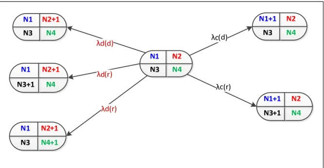
In our case, each state is characterized by a series of four numbers that represent the number of the cellular UE(s) (N1), the number of D2D UE(s) (N2), the number of channels shared with a cellular UE and D2D UE (N3), the number of channels shared with two D2D UEs (N4). The state transition in our case is based on the flows that system has (Arrival rates).Figure2.1 shows how we defined the states.
Figure 2.1 State of Markov chain
Table 1.2 Markov chain’s states parameters
Parameters N1 Number of cellular UE(s)
N2 Number of D2D UE(s)
N3 Number of channels shared with a cellular UE and D2D UE N4 Number of channels shared with two D2D UEs
2.2.2 Possible Actions
The Possible actions (a) in our system are: • Accept Cellular UE in dedicated mode. • Accept D2D connection in dedicated mode.
20
• Accept Cellular UE in reused mode.
• Accept D2D connection in reused mode with cellular UE. • Accept D2D connection in reused mode with D2D UE.
2.2.3 Markov Transition Diagram for Arrival
In the Markov chain, we have a set of possible states. The process starts in one of these states and moves successively from one state to another. We assume that the total numbers of channels is N and each connection occupies one of channels and each channel can be shared by maximum two connections; one cellular UE and one D2D UE or two D2D UEs.
In Markov transition diagram, we have two flows; cellular UEs arrival rate and D2D UEs arrival rate and we assume that each D2D connection has two possible modes; dedicated or reused mode. To make our diagram we use some labels that indicate connection type and selected mode.
Table 2.3 Markov transition diagram labels
Label Connection type TM Served channel
λc(d) Cellular UE Arrival Dedicated Individual channel
λc(r) Cellular UE Arrival Reused Shared channel
λd(d) D2D Arrival Dedicated Individual channel
λd(r) D2D Arrival Reused Shared channel
The Markov transition diagram for arrival is shown in Figure 2.2. Let assume that the current state in the Markov diagram is S with ( N1 , N2 , N3 , N4 ).
21
When a new cellular UE enters and the dedicated mode selects with λc(d) diagram moves to another state has ( N1 + 1, N2 , N3 , N4 ); the number of UE(s) in cellular mode is increased.
If the new cellular UE serves in reused mode diagram moves with λc(r) to state that has ( N1 + 1, N2 , N3 + 1 , N4 ); the number of UE(s) in cellular mode and the number of channels that are shared with a cellular UE and D2D UE are increased.
If new D2D connection enters and is accepted in dedicated mode with λd(d) diagram moves to another state has ( N1 , N2 + 1, N3 , N4 ); the number of D2D UE(s) is increased.
If new D2D connection is accepted in reused mode, they are two possibilities; serves in a channel that already has a cellular UE or serves in a channel that has a D2D UE.
If new D2D connection reuses a channel with a cellular UE with λd(r) diagram moves to another state has( N1 , N2 + 1, N3 + 1 , N4 ); the number of D2D UE(s) is increased and the number of shared channel with cellular UE and D2D UE increased.
If new D2D connection reuses a channel with a D2D UE with λd(r) diagram moves to another state has( N1 , N2 + 1, N3 , N4 + 1); the number of D2D UE(s) is increased and the number of shared channel with two D2D UEs increased.
22
Figure 2.2 Markov transition diagram for arrival
2.2.4 Markov Transition Diagram for Departure
When the service time of connection is finished, the network released it. Figure 2.3 represents the Markov transition diagram for departure.
We assume that the current state in the Markov diagram is S with ( N1 , N2 , N3 , N4 ). When service time of cellular connection in individual mode finished with departure rate of (N1 − N3) × μ diagram moves to another state has ( N1 − 1, N2 , N3 , N4 ). The number of cellular UE(s) is decreased.
If the service time of the of cellular connection in reused mode finished with departure rate of (N3) × μ diagram moves to another state has ( N1 − 1, N2 , N3 −1 , N4 ); The number of cellular UE(s) and the number of shared channels between cellular UE(s) and D2D UE(s) are decreased.
23
If D2D connection with dedicated mode finished diagram moves to another state has ( N1 , N2 − 2, N3 , N4 ) with departure rate (N2 − N3 − 2N4) × μ; the number of D2D UE(s) is decreased.
If service time of the D2D connection in reused mode which used the same channel with a cellular UE finished diagram moves to another state has ( N1 , N2 − 1, N3 − 1 , N4 ) with departure rate (N3) × μ.
If service time of the D2D connection in reused mode that shared with another D2D UE finished diagram moves to another state has ( N1 , N2 − 1, N3 , N4 − 1) with departure rate (2N4) × μ.
24
2.3 Numerical Results
Markov processes are classified into two categories; discrete-time and continuous-time. In our system, the time between state transitions is random variable therefore our system can be modeled in continuous- time.
In many cases, the times between the consecutive decision instances are not identical and random. The semi-Markov decision model can be used to analyze such systems. In this case, most of the characteristics of the semi-Markov decision model are the same as in the discrete case except for the addition of the description of the time between two decision epochs. In particular, when the system arrives at the review time t it is classified into state ∈ . Then a decision is made.
For each state a set of possible actions is , ∈ assumed to be finite. Each action, a, results in a certain reward, ( ), which is given to the system until the next decision epoch. The reward usually consists of a lump reward given at the moment of the decision and a reward rate given continuously in time. In the next time epoch, the system moves to a state which is a function of the transition probabilities ( ) which depend on the taken action in state . Such a system is called a semi-Markov decision model if rewards ( ), transition probabilities ( ) and time until the next decision ( )are independent from the past history of the system.
2.3.1 Possible Actions and Reward Rate
The Possible actions (a) in our system are: • Accept Cellular UE in dedicated mode. • Accept D2D connection in dedicated mode. • Accept Cellular UE in reused mode.
25
• Accept D2D connection in reused mode with D2D UE.
In the diagram, each state has a reward of its own rate and is calculated using the following formula:
( ) = (N ∗ r ) + (N ∗ r ) − 2(N + N ) ∗ C (2.1)
2.3.2 Uniformization Technique
The uniformization technique transforms an arbitrary continuous-time Markov process, which in general can have different average sojourn times in different states, into an equivalent continuous-time Markov process where the average time between transitions is constant. This is done by introducing fictitious transitions between the same states. The rate of transition in equivalent system, , can have any value which satisfies.
≥ , ∈ (2.2)
We have Continues- time Markov decision so to transform it into a discrete Markov chain without losing the information about the state sojourn times. We use the uniformization technique. For two flows of connections ′:
= 1/ (2.3)
= 1
+ + + (2.4)
26
= 1
+ + + 2 (2.5)
2.3.3 Value Iteration Algorithm (VIA)
The value iteration algorithm uses the recursive solution approach from dynamic programming. The VIA evaluates recursively the value function ( ), where = 1,2, …,
( ) = ∈ ( ) + ́
∈
( ) ( ) , (2.6)
The value function is the expected reward from the system and ( ) = ( ) − ( ) is the maximum average reward.
For large n:
∗ = lim
→ [ ( ) − ( )]
(2.7)
The bounds on the ∗ are defined by
= min { ( ) − ( )} (2.8) = max { ( ) − ( )} (2.9)
27
To use VIA for our scenario we apply the uniformization technique. By using the identical transition times = 1/ we convert into a discrete system. We use the value iteration algorithm that presented below for our scenario.
Algorithm 2.1 Value Iteration Algorithm from Dziong (1997, p. 286)
Value Iteration Algorithm – adapted from (Dziong, 1997)
STEP 1. Determine the initial values
{ ( )∶ ∈ , 0 ≤ ( ) ≤ ( )} and = 1. (2.10)
STEP 2. Evaluate the value functions
( ) = ∈ { ́ ( ) + ́
∈
( )[ ( ) − ( )] + ( ) }, ∈ (2.11) And find policy which maximize the right sight of equation 2.11 for all ∈ .
STEP 3. Compute and . If 0 ≤ − ≤ , where determines a
requires relative accuracy, stop algorithm with policy .
STEP 4. Set = + 1 and go to step 2.
28
Figure 2.4 Convergence of value iteration algorithm
2.3.4 Policy Iteration Algorithm
The general goal in MDPs is to get a policy that yields the maximum expected gain over time and policy iteration algorithm is another way to solve reward MDPs such as the value iteration algorithm. It intends to calculate successively policies increasingly well-behaved for MDPs. Policy iteration algorithm starts with a random policy and then calculates its value after that it tries to develop better policy than the previous one. Policy- iteration algorithm does this procedure as far as it obtains a policy that strictly better than the last policy. In the next page, the policy- iteration algorithm is presented.
29
Algorithm 2.2 Policy- Iteration Algorithm Adapted from Dziong (1997, p. 289)
Policy- Iteration Algorithm – adapted from (Dziong, 1997)
STEP 1. Choose an initial stationary policy π.
STEP 2. For given policy π, solve the set of value-determination equations
( ) = ( ) − (π) ( ) + ∑ ∈ ( ) ( ), ∈ (2.12)
By setting the relative value for an arbitrary reference state s to zero.
STEP 3. For each state ∈ find an action producing the maximum in ∈
{ ( ) − (π) ( ) +
( ) ∈
( ) } (2.13) The improved policy is defined = by choosing for all ∈ .
If the improved policy equals the previous policy the algorithm is stopped. Otherwise go to step 2 with replaced by .
In a manner analogous to the discrete case this procedure converge to ∗ in a finite number of iterations.
Observe that by dividing equation 3.1 by ( ) and some simple transformations we can arrive at
= ( ) + ( )[ ∈
( ) − ( ) ], ∈ (2.14) Where ( ) = ( )/ ( ) is the rate of reward. This form of equations can also be used in the policy- iteration algorithm, resulting in the more explicit maximization of the average reward in the policy-improvement step:
∈
{ ( ) +
( )[ ∈
30
2.3.5 Optimal Policy
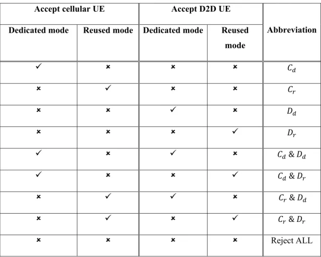
In this section, we present the optimal policy for various reward and cost per connection type. To present the optimal policy we use some colors. In table 2.4, all of the possible actions and their colors are shown.
Table 2.4 Possible actions and their abbreviations in optimal policy
Accept cellular UE Accept D2D UE
Abbreviation
Dedicated mode Reused mode Dedicated mode Reused
mode & & & & Reject ALL
31
• Case 1: =
We assume that the reward rates for cellular and D2D UE(s) are the same and the cost for reused mode is low. The optimal policy for mode selection with these conditions is shown in Figure 2.5.
Figure 2.5 Optimal policy for case 1
Most of the time the network prefers to accept D2D connections in reused mode and cellular UE(s) in dedicated mode. When all of channels are occupied D2D connections accepted in reused mode. 0 1 2 3 4 5 6 7 8 9 10 11 0 1 2 3 4 5 6 7 8 9 10 11
Number of INDIVIDUAL CHANNEL
Nu m b er o f SHA R ED CHAN NEL Accept C
32
• Case 2: =
We assume that the reward rates for cellular and D2D UE(s) are same and the cost for reused mode is high. The optimal policy for mode selection with these conditions is shown in Figure 2.6.
Figure 2.6 Optimal policy for case 2
The network in this case accepts the connections in cellular UE(s) and D2D UE(s) in dedicated mode and when the number of occupied channels increased the total reward for all of modes is close to each other so new cellular connections are in dedicated and D2D UE(s) are in reused mode. 0 1 2 3 4 5 6 7 8 9 10 11 0 1 2 3 4 5 6 7 8 9 10 11
Number of INDIVIDUAL CHANNEL
Nu m b er o f S H AR E D CH A N N E L
33
• Case 3: >
We assume that the reward rate for cellular UE(s) is higher than the reward for D2D UE(s) and the waiting cost is low.
In this case, the network accepts the connections in dedicated mode and then network accepts cellular UE(s) in reused mode and D2D UE(s) in dedicated mode. Figure 2.7 shows the optimal policy for this case.
Figure 2.7 Optimal policy for case 3
• Case 4: >
We assume that the reward rate for cellular UE(s) is higher than the reward for D2D UE(s) and the waiting cost is high.
0 1 2 3 4 5 6 7 8 9 10 11 0 1 2 3 4 5 6 7 8 9 10 11
Number of INDIVIDUAL CHANNEL
Nu m b er o f SHARED CHANNEL
34
In this case, the network accepts cellular UE(s) and most of the channels are assigned to the connections in dedicated mode. Figure 2.8 shows the optimal policy for this case.
Figure 2.8 Optimal policy for case 4
• Case 5: >
We assume that the reward rate for D2D connections is higher than the reward for cellular connection and the waiting cost is low. In this case, the network accepts the connections in dedicated mode and then network accepts cellular UE(s) in dedicated mode and D2D UE(s) in reused mode. Figure 2.9 shows the optimal policy for this case.
0 1 2 3 4 5 6 7 8 9 10 11 0 1 2 3 4 5 6 7 8 9 10 11
Number of INDIVIDUAL CHANNEL
N u m b er o f SHAR E D C HANNEL
35
Figure 2.9 Optimal policy for case 5
• Case 6: >
We assume that the reward rate for D2D connections is higher than the reward for cellular connection and the waiting cost is high.
In this case, the network accepts the connections in dedicated mode and then accepts D2D UE(s) in reused mode and cellular UE(s) in dedicated mode. Figure 2.10 shows the optimal policy for this case.
0 1 2 3 4 5 6 7 8 9 10 11 0 1 2 3 4 5 6 7 8 9 10 11
Number of INDIVIDUAL CHANNEL
Nu m b er o f SH ARED CH ANNEL
36
Figure 2.10 Optimal policy for case 6
2.4 Conclusion
In this chapter, we address the problem of mode selection for D2D enabled 5G networks. We consider a D2D enabled cellular network consisting of D2D UEs and cellular UEs. D2D UEs can operate in the dedicated mode or the reused mode while cellular UEs can be in the cellular mode or in the reused mode with a D2D UE.
We describe how the mode selection can be formulated as an MDP. First, we define four numbers to indicate each state and then we present the Markov chain for our system. To find the optimal mode selection policy we apply the value iteration algorithm and its convergence is presented. 0 1 2 3 4 5 6 7 8 9 10 11 0 1 2 3 4 5 6 7 8 9 10 11
Number of INDIVIDUAL CHANNEL
N u mb er o f S H ARE D CH ANNE L Accept C
37
We present the optimal mode selection policy for six cases. In these cases, we change the reward for cellular UE(s) and D2D UE(s) and the cost for reused mode.
CHAPTER 3
MOBILITY BASED MODE SELECTION ALGORITHM
When connected UEs in a D2D transmission move, the quality of the transmission between the users can be affected. We would like to have a seamless connection with high QoS. For this purpose, we propose a mode selection algorithm that is considering the mobility of UEs.
The chapter begins with a brief problem definition. After that, the QoS parameters are determined and then the mobility models are presented. Then, the Analytic Hierarchy Process (AHP) method is defined. After that, the reward function used for mode selection is proposed. The simulations results and their analysis conclude the chapter.
3.1 Problem Statement
The D2D communication can operate in multiple modes. The cellular network can assign dedicated resources to the D2D terminals, or they can reuse the same resources used by the cellular network. Cellular uplink and downlink communication can facilitate the D2D communication. We consider three D2D communication modes:
• Dedicated mode where the D2D communication is direct and data are transmitted through the D2D link by the orthogonal frequency resources to the cellular users, so there is not any interference.
• Reuse mode where data is transmitted through the D2D link by the reusing the same frequency resources that are considered for a cellular user so reused mode causes interference at receivers. However, the system spectrum efficiency and user access rate may be increased.
40
• Cellular mode where the D2D communication is relayed via eNB and it is treated as cellular users.
The mobility of UEs can change the quality of connection due to changes in the interference then the TM may need to be changed also. The BS has all the involved channel state information available to select the optimal resource-sharing mode between the cellular user and the D2D pair.
We study the problem of the transmission mode change due to, movements of UEs and we seek to have seamless connections that provide the best QoS for UEs in D2D enabled network. For this problem, we need to select the required measured parameters that represent the QoS for each connection and the mobility model should be considered as well.
3.2 Quality of Service
The communication networks support a wide variety of services ranges from voice and data to multimedia services. The service quality requirements from these services are different. Some are sensitive to delays experienced in the communication network, others to loss rates, and others to delay variation. Therefore, the quality of service (QoS) concept is becoming an ever more critical issue in the telecommunication (Al-Shaikhli, 2015).
3.3 QoS Parameters
The main QoS parameters considered in telecommunication networks are delay, throughput and bandwidth.
• Delay
Delay is an essential parameter in telecommunication because the information should transmit between two points and it takes time to reach another side. End-to-end delay or one-way delay
41
is the total time that information is sent to destination. The one-way delay from source to destination plus the delay from destination to the source is called round-trip delay. In our problem, we considered one-way delay for each connection, and we would like to reduce it. • Bandwidth
Bandwidth management depends on the type of the service that the user is using and policy rules that predefined to manage available bandwidth. The minimum bandwidth, maximum bandwidth, priority and parent designation are four parameters for bandwidth classes. The minimum bandwidth factor shows the guaranteed bandwidth for service and maximum bandwidth limits the amount of bandwidth for a kind of service also the classes of services can be prioritized, and specific class can receive bandwidth before than others as well to prioritization and defining the bandwidth limits a class hierarchy should be used. Class hierarchy determines classes’ priority and the maximum or minimum bandwidth requirements (Al-Shaikhli, 2015).
• Throughput
The overall throughput for each mode is almost equal to the network’s overall capacity and equations in below show the throughput for cellular, dedicated and reused modes. The subscripts s, c, d and e stand for source UE( ) , cellular UE ( ) , destination UE( ) , and eNB respectively. Other parameters are presented in table 3.1.
42
Table 3.1 Parameters for throughput formulation
Parameters Definition
Overall throughput of the network in reused mode Overall throughput of the network in dedicated mode Overall throughput of the network in cellular mode ℎ Channel gain between transmitter i and receiver j
Transmit power of i = log (1 + | | | | ) + log (1 + | | | | ) (3.1) = log (1 + | | | | ) + log (1 + | | | | ) (3.2)
= log (1 + | | ) , log (1 + | | ) + log (1 + | | ) (3.3)
Where the channel gain is calculated as equation 3.4:
ℎ = (3.4)
Where K is a unitless constant that depends on antennas characteristics and a is the path loss exponent. The is the distance between transmitter i and receiver j. The transmitter can be s,c or e and j can be e or d (Morattab, 2016).
43
3.4 Mobility Model
In the D2D communication, the mobile nodes can be connected directly to other nodes or they can use the cellular transmission mode. If the mobile nodes are independent of each other, we define the entity mobility model for them. On the other side, if they are dependent on each other we define the group mobility model for them.
Generally, for simulation the mobility models of the mobile node we consider two factors: speed and direction. After the T time or D distance, the mobile nodes change the speed and direction (Hong, 1999).
In this work, we consider four entity mobility models that are presented in the next section.
3.4.1 Random Walk Mobility Model
In this model, the mobile node chooses the random speed and direction and after constant time T or constant distance D the new speed and direction are chosen again. The speed range is [speed min, speed max] and direction range is [0,2π] (Hong, 1999).
44
3.4.2 Random Waypoint Mobility Model
Random waypoint mobility model has pause time it means that the mobile node before chooses the new speed and direction has a constant pause time. If the pause time is set to the zero this mobility model is similar to the Random walk mobility model (Hong, 1999).
3.4.3 Random Direction Mobility Model
In the random direction model, the mobile node considers the border of the simulation area as the distention and travel to them and when it reached the border it pauses for the specified time, chooses another direction and continues the process (Hong, 1999).
Figure 3.2 Random Direction Mobility Model
3.4.4 Random Waypoint - Cell wrapped Mobility Model
In Random Waypoint - Cell wrapped Mobility Model, the mobile user chooses the random speed and direction and after constant time T or constant distance D the new speed and direction are chosen again. The speed range is [speed min, speed max] and direction range is [0,2π]. When the mobile user reaches the edge of cell it enters the cell from another side of the cell (Hong, 1999).
45
Figure 3.3 Random Waypoint - Cell wrapped Mobility Model
3.5 Analytic Hierarchy Process (AHP) method
The Analytic Hierarchy Process (AHP) is a multi-criteria decision making. The AHP is a decision support tool which can be used when multiple and conflicting objectives and criteria are present. It uses a multi-level hierarchical structure of objectives, criteria, sub-criteria, and alternatives and it generates a weight for each evaluation criterion (Yu, 2002).
In our case, the criteria and sub-criteria are QoS parameters and velocity of user. Figure 3.4 represents hierarchical decomposition of criteria.
46
Figure 3.4 Hierarchical decomposition of criteria
According to the hierarchical decomposition, the total importance of QoS parameters are equal to rate and velocity parameters because delay and bandwidth are in the second level.
3.6 Reward Function
In this section, we define the total reward function by considering the QoS parameters and user’s velocity also we will use the AHP to add the weight for the criteria.
• Delay function
As the delay for transmission mode a is d the delay reward function is defended as equation 4.5: ( , ) = 1, 0 < ≤ ( − ) ( − ) , < < 0, ≤ (3.5)
47
Where d is the delay for mode a and U and L are the maximum and minimum delay requirements.
• Bandwidth function
When the total available bandwidth for the user is the bandwidth reward function is defined as ( , ) = 1, ≥ ( − ) ( − ) , < < 0, ≤ (3.6)
Where L and U denote the minimum and maximum bandwidth requirements of user.
• Throughput reward function
When the throughput for mode a is the throughput reward function is defined as
( , ) =
−∞ <
1 > (3.7) Where represent the threshold for mode a.
• Connection dropping penalty function We defined the call dropping penalty function as
( , ) = , ≤ ≤ −∞, > (3.8)
Where the and are the maximum and minimum velocity thresholds of user and v is the current velocity of user. When the mobile user is moving fast the probability of dropping