C
⃝2014. The American Astronomical Society. All rights reserved. Printed in the U.S.A.
CONSTRAINING THE EXOZODIACAL LUMINOSITY FUNCTION OF MAIN-SEQUENCE STARS:
COMPLETE RESULTS FROM THE KECK NULLER MID-INFRARED SURVEYS
B. Mennesson1, R. Millan-Gabet2, E. Serabyn1, M. M. Colavita1, O. Absil3, G. Bryden1, M. Wyatt4, W. Danchi5,
D. Defr`ere6, O. Dor´e1, P. Hinz6, M. Kuchner5, S. Ragland7, N. Scott8, K. Stapelfeldt5, W. Traub1, and J. Woillez9
1Jet Propulsion Laboratory, California Institute of Technology, 4800 Oak Grove Drive, Pasadena, CA 91109-8099, USA;Bertrand.Mennesson@jpl.nasa.gov 2NASA Exoplanet Science Center, California Institute of Technology, 770 South Wilson Avenue, Pasadena, CA 91125, USA
3D´epartement d’Astrophysique, G´eophysique et Oc´eanographie, Universit´e de Li`ege, 17 All´ee du Six Aoˆut, 4000 Li`ege, Belgium 4Institute of Astronomy, University of Cambridge, Madingley Road, Cambridge CB3 0HA, UK
5NASA Goddard Space Flight Center, Exoplanets and Stellar Astrophysics Laboratory, Code 667, Greenbelt, MD 20771, USA 6Steward Observatory, Department of Astronomy, University of Arizona, 933 N. Cherry Avenue, Tucson, AZ 85721, USA
7Keck Observatory, 65-1120 Mamalahoa Highway, Kamuela, HI 96743, USA
8Center for High Angular Resolution Astronomy, Georgia State University, Mount Wilson, CA 91023, USA 9European Southern Observatory, Karl-Schwarzschild-Strasse 2, D-85748 Garching bei Munchen, Germany
Received 2014 July 5; accepted 2014 October 1; published 2014 December 8
ABSTRACT
Forty-seven nearby main-sequence stars were surveyed with the Keck Interferometer mid-infrared Nulling instrument (KIN) between 2008 and 2011, searching for faint resolved emission from exozodiacal dust. Observations of a subset of the sample have already been reported, focusing essentially on stars with no previously known dust. Here we extend this previous analysis to the whole KIN sample, including 22 more stars with known near- and/or far-infrared excesses. In addition to an analysis similar to that of the first paper of this series, which was restricted to the 8–9 µm spectral region, we present measurements obtained in all 10 spectral channels covering the 8–13 µm instrumental bandwidth. Based on the 8–9 µm data alone, which provide the highest signal-to-noise measurements, only one star shows a large excess imputable to dust emission (η Crv), while four more show a significant (>3σ ) excess: β Leo, β UMa, ζ Lep, and γ Oph. Overall, excesses detected by KIN are more frequent around A-type stars than later spectral types. A statistical analysis of the measurements further indicates that stars with known far-infrared
(λ! 70 µm) excesses have higher exozodiacal emission levels than stars with no previous indication of a cold outer
disk. This statistical trend is observed regardless of spectral type and points to a dynamical connection between the inner (zodi-like) and outer (Kuiper-Belt-like) dust populations. The measured levels for such stars are clustering close to the KIN detection limit of a few hundred zodis and are indeed consistent with those expected from a population of dust that migrated in from the outer belt by Poynting–Robertson drag. Conversely, no significant mid-infrared excess is found around sources with previously reported near-mid-infrared resolved excesses, which typically have levels of the order of 1% over the photospheric flux. If dust emission is really at play in these near-infrared detections, the absence of a strong mid-infrared counterpart points to populations of very hot and small (submicron) grains piling up very close to the sublimation radius. For solar-type stars with no known infrared excess, likely to be the most relevant targets for a future exo-Earth direct imaging mission, we find that their median zodi level is 12 ± 24 zodis and lower than 60 (90) zodis with 95% (99%) confidence, if a lognormal zodi luminosity distribution is assumed.
Key words: circumstellar matter – infrared: stars – instrumentation: interferometers
Online-only material:color figures
1. INTRODUCTION
Debris disks found around main-sequence stars are the remnants of planetary formation. The outer colder parts of these disks, analogous to our solar system Kuiper–Edgeworth (hereafter Kuiper) Belt, were first detected via their mid-infrared (MIR) or far-mid-infrared (FIR) excess emission and then imaged at visible to submillimeter wavelengths. Structures and asymmetries in spatially resolved debris disks have been used to infer the presence of yet unseen planets. The power of this technique was recently demonstrated with the direct imaging of a massive planet at the inner edge of the warped extended
dust disk previously detected around β Pic (Lagrange at al.2009;
Macintosh et al.2014). Conversely, very little is known about the
hotter (>200 K) dust component of debris disks, concentrated in the inner few AU of the stellar environment where rocky planets may have formed, similar to the zodiacal dust found in the inner solar system, which originates from the tails of comets and from collisions between asteroids in the asteroid belt.
Indeed, only a few hot debris disks have been found by Spitzer around mature stars from excess emission at wavelengths of
24 µm or shorter (Beichman et al.2006a; Lawler et al.2009),
and only a few have been unambiguously resolved so far (e.g.,
Smith et al. 2009). This observational difficulty results from
two main factors: the exozodiacal disks’ small angular sizes, and their faintness relative to the host star. Indeed, while cold debris disks cause very significant excesses readily detectable at FIR wavelengths, exozodiacal material located in the inner few AU only contributes a small fraction of the stellar MIR flux. In order to reliably detect such tiny (≃1%) excess emis-sion over that expected from the photosphere, direct imaging is required, with the ability to spatially resolve dust from the central star. In the visible, where dust is seen by means of scattered starlight, the contrast required is extremely high and only a space- or balloon-borne coronagraph could provide ad-equate performance. In the infrared, exozodiacal disks produce significant thermal emission and contribute a larger fraction of the stellar flux, making it the spectral range of choice for
ground-based exozodiacal studies. With the spatial scales at play, typically 0.1 to a few AU, such direct infrared observations are best accomplished using long-baseline interferometry. This was the main goal of the Keck Interferometer Nuller (KIN), a long-baseline (85 m), high-contrast instrument operating be-tween 8 and 13 µm, especially built to spatially resolve faint
structures next to bright stars (Serabyn et al.2012; Colavita et al.
2013). Exozodiacal observations were carried out with the KIN
between 2008 and 2011 through three different Key Science pro-grams (led by Serabyn, Hinz, and Kuchner, respectively) and one PI program (led by Mennesson). These studies targeted a total of 47 nearby main-sequence stars whose basic properties are listed
in Table1. We already analyzed a subset of this sample
(Millan-Gabet et al.2011, hereafter Paper I) comprising 23 stars with
no previously known dust and 2 with dust previously detected
in the MIR and FIR: η Crv (Beichman et al.2006b; Chen et al.
2006; Smith et al.2009) and γ Oph (Su et al.2008). This initial
data analysis was restricted to a single spectral channel spanning 8–9 µm and revealed only one clear excess (around η Crv) and two marginal ones (around γ Oph and Altair). It also provided the best limits to date on 10 µm exozodi levels for a sample of nearby main-sequence stars, with a typical measurement uncer-tainty (1σ ) of 150 times the solar zodiacal light emission, or 150 “zodis.” For all stars in our sample, we define the unit zodi case as a dust cloud with the same optical depth at 1 AU and the same radial density profile as measured in the solar system (Kelsall
et al.1998), but with an inner dust radius and radial temperature
profile that scale with stellar luminosity (see Section3.5 for
further details).
In this context, our present goals are to (1) perform a final calibration of the complete KIN sample of 47 stars using a consistent set of rules for data vetting, calibrator diameters, and uncertainties; (2) compute all individual star excess mea-surements over the full 8–13 µm spectral range, divided into 10 spectral channels; (3) assess possible correlations between basic stellar properties and measured MIR excesses; and (4) derive conclusions on the prevalence of high levels of exozodi emission for nearby Sun-like stars. As the more sensitive Large Binocular Telescope Interferometer (LBTI) exozodi survey is just starting, it is also timely to draw a final set of conclusions from the KIN surveys to help refine the LBTI stellar sample
selection (Weinberger et al.2014).
2. CALIBRATION AND DATA VETTING
The KIN data acquisition principle and reduction technique
are fully described in past publications (Colavita et al.2009;
Millan-Gabet et al. 2011; Serabyn et al. 2012) and will not
be discussed in detail here. Similar to regular interferometric observations, the correction of instrumental effects is based on interspersed nulling observations of science targets and nearby calibrator stars. These calibrators have well-known diameters and are used to derive accurate estimates of the instrumental leakage at the time of science target observations.
2.1. Calibrators
In order to minimize systematic errors in the calibration, cal-ibrator stars were chosen close to the science targets and with similar MIR fluxes. As a result, these calibrator stars were typ-ically giants. In order to most accurately predict their angular diameters, we retained only the observations of giant calibra-tors with spectral types G, K, and early M. We also made a thorough check through the literature and rejected any
cali-brator with a reference to possible binarity or variability. As
stated in Paper I, these different criteria minimize the
possi-bility of infrared emission above photospheric levels (Cohen
et al.1999).10 The calibrators’ limb-darkened (LD) diameters
were computed adopting the following set of rules:
1. If a calibrator was listed in the Bord´e et al. (2002) or
Merand et al. (2006) catalogs of interferometric
calibra-tors, we adopted its estimated LD diameter, with a relative error bar of ±5%. This error is conservatively increased in comparison to the catalog’s quoted uncertainties (typi-cally 1.5%), reflecting the typical offset measured with re-spect to long-baseline interferometric measurements when available.
2. Otherwise, we used surface brightness relations,
specifi-cally the LD diameter versus (V0− K0) relation, where V0
and K0 are the measured V and K magnitudes corrected
for interstellar extinction. We assumed the extinction to be isotropic, i.e., just a function of stellar distance. Because common surface brightness relations are valid over spe-cific ranges of color differences, we then considered two subcases:
(a) If the derived V0 − K0 was between −0.1 and 3.6,
we used the surface brightness relationship established
by Di Benedetto (2005, Equations (2) and (4)). We
then applied an LD diameter error bar of ±6% if the K magnitude came from Two Micron Sky Survey Infrared
catalog (TMSS; Neugebauer & Leighton1969) or from
JP11 (IRAS catalog; Gezari et al.1993) measurements.
We used an error bar of ±10% if the K magnitude came from the Two Micron All Sky Survey (2MASS), whose measurements are saturated and fairly inaccurate for our bright calibrators.
(b) If the derived V0 − K0 was between 3.6 and 7 or
between −1.1 and −0.1, we used the surface
bright-ness relationship established by Bonneau et al. (2006,
Equations (9) and (10) and Table 2 of that paper), in the case of bright objects (V < 10, K < 5). We applied an error bar of ±7% if the K magnitude came from TMSS or JP11 measurements. We used an error bar of ±10% if the K magnitude came from 2MASS. The error bars quoted above (6%, 7%, or 10%) were derived by comparing the derived surface brightness LD diameters with
those estimated by Bord´e et al. (2002) and Merand et al. (2006)
for an ensemble of 100 calibrators (including those used in this work), assuming that the Bord´e and Merand values were “the correct ones.” It is worth noting that calibrator diameters
were estimated in a different way inPaper I, which used Keck
Interferometer K-band measurements acquired at the same time as the MIR null measurements. The present calibration strategy leads to slightly revised null values for the 25 science targets
already discussed inPaper I. However, all changes are within the
calibrated null error bars of a few times 10−3, with the exception
of Altair (see Section5.2).
2.2. Data Vetting
For each science target, we only retained null data sequences (or “scans”) based on the following criteria: at least one calibrator observation is available within 1 hr, and the percentage
10 If there was any significant N-band excess emission around the calibrators,
this would bias the science target measurements toward lower or even negative null excess levels, which we do not observe.
Table 1
Target Properties and Observing Log
HD Star Spectral Object Lstar/L⊙ Rstar/R⊙ Tstar Fstar LD Diam IWA OWA R300 K Nc Dates Ns
Type Type (K) (Jy) (mas) (AU) (AU) (AU) (UT)
432 βCas F2IV ecold 27.3 3.4 7079 15.3 2.027 ± 0.122 0.10 3.4 5.2 2 2008 Aug 17 3
N/A ηCas A G3 · · · 1.3 1.0 6087 9.8 1.894 ± 0.114 0.04 1.2 1.1 2 2010 Sep 22 3
9826 υAnd F9V · · · 3.3 1.6 6120 3.9 1.021 ± 0.060 0.08 2.7 1.8 1 2008 Nov 12 2
10476 107 Psc K1V · · · 0.4 0.8 5180 2.6 1.067 ± 0.064 0.04 1.5 0.7 2 2008 Oct 13 2 10700 τCeti G8V eboth 0.5 0.8 5344 11.8 2.015 ± 0.023 0.02 0.7 0.7 5 2008 Oct 14 4 2008 Oct 15 2 13161 βTri A5III bin3 71.0 4.4 8020 4.7 1.050 ± 0.100 0.23 7.8 8.4 2 2008 Aug 18 1
13974 δTri G0V bin3 1.1 1.0 5860 2.7 1.105 ± 0.111 0.07 2.2 1.0 2 2008 Nov 13 2
16895 θPer F7V · · · 2.2 1.2 6320 4.0 1.086 ± 0.056 0.07 2.2 1.5 3 2009 Jan 11 2
2009 Jan 12 1
19373 ιPer F9V · · · 2.2 1.4 5890 4.7 1.086 ± 0.056 0.06 2.1 1.5 4 2009 Jan 11 1
20630 κ-1 Cet G5V · · · 0.8 1.0 5620 2.7 0.895 ± 0.070 0.05 1.8 0.9 2 2009 Jan 10 1
22049 ϵEri K2V ecold 0.3 0.7 5084 12.2 2.126 ± 0.131 0.02 0.6 0.5 3 2008 Oct 13 2
2008 Oct 14 3 2009 Jan 13 1
22484 10 Tau F8V eboth 3.0 1.6 5981 3.7 1.130 ± 0.068 0.08 2.8 1.7 3 2011 Feb 14 2
30652 1 Ori F6V · · · 2.6 1.3 6450 7.9 1.409 ± 0.050 0.05 1.6 1.6 3 2008 Feb 17 3
2008 Feb 18 1 34411 λAur G1IV-V · · · 1.7 1.3 5820 2.7 0.940 ± 0.056 0.08 2.5 1.3 2 2009 Jan 12 1
38393 γLep F6V · · · 2.3 1.2 6410 5.9 1.871 ± 0.112 0.05 1.8 1.5 3 2009 Jan 10 1
2009 Jan 13 1 38678 ζLep A2IV-V ecold 14.0 1.5 9772 2.6 0.670 ± 0.140 0.13 4.3 3.7 5 2008 Nov 12 2 2009 Jan 9 1 2009 Jan 12 1 2009 Jan 13 1 2011 Feb 14 1
39587 χ-1 Ori G0V bin1 1.0 1.0 5930 3.6 1.124 ± 0.057 0.05 1.7 1.0 4 2009 Jan 10 2
2009 Jan 13 2
40136 ηLep F2V eboth 4.6 1.5 6900 3.7 0.987 ± 0.059 0.09 3.0 2.1 4 2009 Jan 9 3
2009 Jan 10 1 2009 Jan 13 1
56537 λGem A3V ehot 27.8 2.0 9380 2.6 0.644 ± 0.006 0.19 6.2 5.3 2 2010 Sep 22 2
88230 NSV 4765 K8V · · · 0.1 0.8 3920 3.1 1.238 ± 0.054 0.03 1.0 0.4 2 2009 Jan 10 1
95128 47 UMa G1V · · · 1.6 1.2 5860 2.0 0.774 ± 0.073 0.08 2.8 1.2 4 2009 Jan 10 1
2009 Jan 11 1
95418 βUma A1V ecold 63.0 3.0 9377 6.0 1.078 ± 0.065 0.15 4.9 7.9 2 2008 May 26 2
2008 May 27 2 95735 HIP 54035 M2V · · · 0.025 0.3 3730 3.2 1.439 ± 0.050 0.02 0.5 0.1 1 2008 Apr 14 2 2009 Jan 10 1 102647 βLeo A3V eboth 15.0 1.7 8500 9.1 1.339 ± 0.087 0.07 2.2 3.9 2 2008 Feb 18 2 2008 Apr 16 3 2009 Jan 11 1
102870 βVir F9V · · · 3.4 1.7 6080 6.6 1.431 ± 0.086 0.07 2.2 1.9 3 2008 Feb 17 2
2008 Feb 18 4 106591 δUma A3V ecold 14.0 1.4 9480 3.0 0.823 ± 0.049 0.15 4.9 3.7 4 2008 Apr 16 3 2009 Jan 10 1
109085 ηCrv F2V ecold 4.7 1.5 6870 2.5 0.833 ± 0.050 0.11 3.6 2.2 5 2008 Apr 17 1
2008 May 24 3
114710 βCom G0V · · · 1.3 1.1 5960 3.8 1.071 ± 0.058 0.05 1.8 1.2 3 2008 Feb 16 3
115617 61 Vir G7V ecold 0.9 1.0 5577 3.2 1.164 ± 0.116 0.05 1.7 0.9 3 2009 Jan 12 3 117176 70 Vir G5V ecold 3.1 1.9 5545 2.8 0.953 ± 0.062 0.11 3.6 1.8 5 2008 Apr 15 1 2008 Apr 17 3 2009 Jan 13 2
120136 τBoo F6IV bin1 3.0 1.4 6370 2.5 0.864 ± 0.066 0.09 3.1 1.7 2 2008 May 25 3
2008 May 27 2 131977 KX Lib K4V · · · 0.3 0.8 4570 3.1 1.490 ± 0.089 0.04 1.2 0.5 2 2008 May 26 2 142091 κCrb K1IV eboth 12.9 5.0 4877 5.5 1.550 ± 0.093 0.19 6.2 3.6 1 2011 Jun 25 2 142860 γSer F6IV · · · 2.7 1.4 6370 4.7 1.161 ± 0.055 0.07 2.2 1.7 2 2008 Apr 16 3 2008 Apr 17 2 161868 γOph A0V ecold 21.9 1.9 9030 1.8 0.630 ± 0.063 0.17 5.8 4.7 4 2008 Jul 16 3 2008 Jul 17 3 165341 70 Oph K0V · · · 0.6 1.0 5140 9.8 2.037 ± 0.122 0.03 1.0 0.8 1 2008 Aug 17 2 2008 Aug 18 2 172167 Vega A0V eboth 40.1 2.4 9602 53.9 3.306 ± 0.030 0.05 1.5 6.3 9 2008 May 27 4 2008 Jul 14 1
Table 1
(Continued)
HD Star Spectral Object Lstar/L⊙ Rstar/R⊙ Tstar Fstar LD Diam IWA OWA R300 K Nc Dates Ns
Type Type (K) (Jy) (mas) (AU) (AU) (AU) (UT)
2008 Jul 15 4 2008 Aug 15 2 2008 Aug 16 7
177724 ζAql A0V ehot 39.0 2.3 9620 3.6 0.888 ± 0.136 0.15 5.1 6.2 2 2010 Sep 22 3
187642 Altair A7V ehot 10.6 1.6 6900 46.1 3.640 ± 0.030 0.03 1.0 3.3 4 2008 May 25 2 2008 May 26 3 2011 Jun 25 3 201091 61 Cyg A K5V bin3 0.2 0.7 4300 6.7 1.775 ± 0.013 0.02 0.7 0.4 2 2008 Aug 17 3 203280 αCep A7IV ehot 17.0 2.3 7740 9.3 1.577 ± 0.095 0.09 3.0 4.1 2 2010 Sep 21 2
210027 ιPeg F5V bin2 3.3 1.4 6540 4.8 1.070 ± 0.100 0.07 2.4 1.8 2 2008 Jul 14 2
216956 αPsa A4V eboth 16.6 1.8 8590 21.9 2.223 ± 0.022 0.05 1.5 4.1 3 2008 Jul 16 4 2008 Jul 17 4
222368 ιPsc F7V · · · 3.3 1.6 6240 3.9 1.062 ± 0.135 0.08 2.8 1.8 4 2008 Oct 13 2
19356 βPer B8V bin4 98 3.0 11400 9.4 1.350 ± 0.100 0.07 2.2 11.7 3 2008 Oct 15 3
2008 Oct 16 2
83808 14 Leo A5V bin4 11.6 1.7 8180 5.3 1.347 ± 0.081 0.24 8.0 3.4 4 2008 Feb 16 2
2008 Feb 17 3 2008 Apr 14 4
139006 αCrb F0V bin4 5.8 1.5 7300 6.9 1.202 ± 0.056 0.14 4.6 2.4 4 2008 Apr 14 4
2008 Apr 15 3 2008 Jul 13 4
Notes. List of KIN targets sorted by increasing right ascension. Object type indicates any peculiarity about the target. “bin 1”: binary system with companion outside
of KIN FOV. “bin 2”: binary system with companion of known properties within the KIN FOV and no obvious signature in the null measurements. “bin 3”: binary system with companion of unknown brightness and no obvious signature within the KIN FOV. “bin4”: binary system with companion inside the KIN FOV and some obvious signature in the null measurements. No zodiacal-level estimation was possible for these three “bin 4” stars, which are listed separately at the end of the table. “ecold”: cold excess previously detected at MIR or FIR wavelengths. “ehot”: hot excess previously detected in the NIR. “eboth”: both cold and hot excess previously detected. Fstar: 10 µm stellar flux in Jy. LD Diam: stellar LD diameter in mas. IWA/OWA: KIN inner and outer working angles (in AU). R300 K: minimum distance
for 300 K dust (in AU). Nc: total number of calibrator stars used. Ns: total number of null data sequences recorded.
of gated data (Colavita et al. 2009) retained for that scan
is greater than 50%, indicating reasonably good phase and angle tracking performance. We also checked that the nightly log sheets reported adequate observing conditions in terms of cloud cover and seeing, no instrumental configuration change or realignment between target and calibrator, no evidence for fast photometry dropouts, and no major issues with the atmospheric dispersion correctors (ADCs). Namely, we removed all scans with large sudden jumps or saturation (hard limit reach) of the ADC prism’s position, indicating strongly variable or poor instrumental nulls.
3. RESULTS
3.1. Excess Leak Curves
As described in Paper I and in Serabyn et al. (2012),
the quantity observed by the KIN may be understood by projecting the fringe pattern on the sky: what is measured is the astrophysical flux from the object’s surface brightness transmitted through a four-beam nuller fringe pattern (see
AppendixAfor a complete description). For the work presented
here, we measure and calibrate the transmitted flux (expected to be small) due to dust surrounding the central target stars. Thus, we refer to the basic observable as the flux leakage or simply the “leak.” The amount of flux leakage not attributable to the finite size of the central stars is referred to as “excess leak,” and by measuring it we can learn about the amounts of circumstellar dust present. The data reduction steps defined hereafter were applied to all 47 science targets and are identical for all 10 spectral channels covering the full 8–13 µm bandwidth of the instrument. Additionally, the real-time archiver saves the signal
summed over the two spectral channels between 8 and 9 µm,
forming the so-called 8–9 µm null bin already used inPaper I,
which is treated here as an “11th” channel.
1. For each individual stellar scan (typically 5 minutes long), we computed a raw leak (observed null depth) versus wavelength.
2. We then subtracted the instrumental leakage measured on nearby calibrators, which yields the target’s calibrated leak versus wavelength.
3. Owing to their finite extension, all targets observed are slightly resolved by the KIN. In the case of a photosphere
represented by an LD disk of diameter θLD with a linear
LD coefficient uλ, the corresponding stellar leak is given
by (Absil et al.2006,2011) Lstar(λ) = ! π BθLD 4λ "2 ! 1 − 7uλ 15 " # 1 − uλ 3 $−1 . (1)
When working in the MIR, LD effects are generally small (<0.1) for main-sequence stars. As a result, we generally
assume uλ = 0 in the equation above. As long as the
linear LD coefficient is smaller than 0.1, this approximation
translates into a stellar leak error of a few times 10−4
at most, which is completely negligible compared to our measurement uncertainty. The only two exceptions are
Vega and Altair (see Section5.2). Both are rapid rotators
with significant—gravity induced—LD and large enough diameters that this effect must be taken into account when computing the stellar leak. For Vega, we adopted the
β Cas - F2IV (ecold) 8 9 10 11 12 13 Wavelength (µm) -0.010 -0.005 0.000 0.005 0.010 0.015 0.020
average excess leak
η Cas A - G3 8 9 10 11 12 13 Wavelength (µm) -0.02 -0.01 0.00 0.01 0.02 0.03 0.04
average excess leak
υ And - F9V 8 9 10 11 12 13 Wavelength (µm) -0.06 -0.04 -0.02 0.00 0.02 0.04 0.06
average excess leak
107 Psc - K1V 8 9 10 11 12 13 Wavelength (µm) -0.02 0.00 0.02 0.04 0.06 0.08 0.10 0.12
average excess leak
τ Ceti - G8V (eboth) 8 9 10 11 12 13 Wavelength (µm) -0.03 -0.02 -0.01 0.00 0.01
average excess leak
β Tri - A5III (bin3)
8 9 10 11 12 13 Wavelength (µm) -0.05 0.00 0.05 0.10 0.15
average excess leak
δ Tri - G0V (bin3) 8 9 10 11 12 13 Wavelength (µm) -0.14 -0.12 -0.10 -0.08 -0.06 -0.04 -0.02 0.00 0.02
average excess leak
θ Per - F7V 8 9 10 11 12 13 Wavelength (µm) -0.04 -0.02 0.00 0.02 0.04
average excess leak
ι Per - F9V 8 9 10 11 12 13 Wavelength (µm) -0.02 0.00 0.02 0.04 0.06 0.08 0.10 0.12
average excess leak
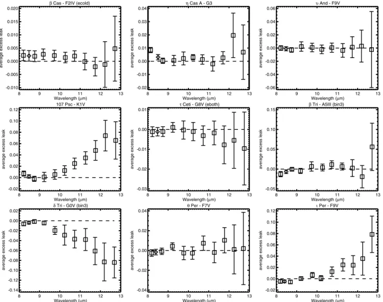
Figure 1. Excess leaks measured as a function of wavelength for 44 stars with no obvious stellar companion signature in the data (displayed in the same—increasing
right ascension—order as in Table1). All available measurements are averaged together to produce the curves displayed. This sample includes 38 presumably single stars, 2 stars with known stellar companions outside of the KIN FOV (type “bin1”), and 4 stars with known stellar companions within the KIN FOV (binary types “bin2” and “bin3”). The designations “ecold,” “ehot,” and “eboth” correspond to stars with known cold excess (λ = 60–160 µm), hot excess (around 2 µm), or both types of excess, respectively. The degradation of sensitivity at the red end of the bandpass, as discussed in the text, can be clearly seen. For the analysis presented in this paper, we use both the excess measured in the 8–9 µm spectral bin (filled diamonds), which has the highest sensitivity for exozodi detection, and broadband excess estimates based on the whole 8–13 µm range.
θLD = 3.329 ± 0.03 mas and uλ = 0.10 between 8 and
13 µm. For Altair, we adopted for each KIN observation the position angle (P.A.) dependent diameter measured by
Monnier et al. (2007) with the CHARA interferometer.
At each wavelength and for each individual scan, the stellar leak is then subtracted from the calibrated leak defined above, yielding the measured excess leak versus wavelength.
4. A single measured excess leak versus wavelength curve is then computed per target, averaging all scans (typically between 1 and 4) obtained under a common set of instru-mental conditions, which we refer to as an observational
“cluster.”11Say that a given cluster (index j) consists of a
set of individual scans (index i) characterized at any
sin-gle wavelength by an excess leak measurement Eij with
uncertainty σij. The average excess leak Ejcorresponding
11 Unless a major optical realignment occurred during the observations (e.g.,
caused by a change of the static delay line position), there is only one observational cluster per night and per target.
to that cluster is computed as the weighted least-squares mean from individual scans:
Ej = % iEij/σij2 % i1/σij2 . (2)
5. The uncertainty on the cluster excess leak is estimated
by computing a statistical “internal” term σint
j , decreasing
with the number of scans but still nonzero if all noisy measurements happen to be equal to
σjint= &%1
i1/σij2
, (3)
and a second “external” error σext
j that reflects the scatter
of individual measurements (weighted standard deviation),
σjext= ' ( ( ) % i(Eij − Ej)2/σij2 % i1/σij2 . (4)
κ-1 Cet - G5V 8 9 10 11 12 13 Wavelength (µm) -0.15 -0.10 -0.05 0.00 0.05 0.10
average excess leak
ε Eri - K2V (ecold) 8 9 10 11 12 13 Wavelength (µm) -0.010 -0.005 0.000 0.005 0.010
average excess leak
10 Tau - F8V (eboth) 8 9 10 11 12 13 Wavelength (µm) -0.05 0.00 0.05 0.10
average excess leak
1 Ori - F6V 8 9 10 11 12 13 Wavelength (µm) -0.02 0.00 0.02 0.04 0.06
average excess leak
λ Aur - G1IV-V 8 9 10 11 12 13 Wavelength (µm) -0.15 -0.10 -0.05 0.00 0.05
average excess leak
γ Lep - F6V 8 9 10 11 12 13 Wavelength (µm) -0.02 0.00 0.02 0.04 0.06
average excess leak
ζ Lep - A2IV-V (ecold)
8 9 10 11 12 13 Wavelength (µm) -0.02 0.00 0.02 0.04 0.06
average excess leak
χ-1 Ori - G0V (bin1) 8 9 10 11 12 13 Wavelength (µm) -0.03 -0.02 -0.01 0.00 0.01 0.02 0.03
average excess leak
η Lep - F2V (eboth) 8 9 10 11 12 13 Wavelength (µm) -0.08 -0.06 -0.04 -0.02 0.00 0.02
average excess leak
Figure 1. (Continued) Both internal and external uncertainties are taken into
ac-count and summed in quadrature. The resulting uncertainty
is then compared to the systematic error floor σsysper
clus-ter recommended in Table 2 of Colavita et al. (2009), which
is a function of wavelength and stellar flux. Only the larger value is retained, and the final leak excess uncertainty per cluster is hence defined as
σj = max
!&*
σjint+2+*σjext+2, σsys
"
. (5)
6. Finally, in the case where several data clusters are available for a given target, a weighted mean excess leak is computed for each wavelength as
E= % jEj/σj2 % j1/σj2 , (6)
and its uncertainty is estimated as
σ = &%1
j1/σj2
. (7)
As a summary, the final KIN data reduction products consist of stellar excess leak curves measured as a function of wavelength.
As described in Paper I, in the usual case that the MIR
circumstellar (exozodiacal) flux is small compared to the stellar photospheric flux, the excess leak (E) is proportional to the MIR flux emitted by the exozodiacal cloud, expressed as a fraction of the stellar flux. The proportionality factor is the transmission by the sky-projected KIN null fringe pattern, which is discussed in the next section. Thus, for a point-source star with no circumstellar material, we would measure
E= 0, and this fraction increases as more exozodiacal emission
is spatially resolved. KIN measured excess leak curves are accessible either per individual scan, per cluster (averaging several scans gathered within a single night), or by averaging data from different clusters/observing nights, when applicable. Excess leaks were computed for all 47 targets observed. For
44 of them (Figure 1), little or no significant fluctuation is
detected between the different scans and all available data are averaged together as described above. The remaining three targets are small-separation multiple-star systems exhibiting large null variation versus time as the projected baseline or the companion position varies. In those cases, we show individual
scan results (Figure2) rather than temporal averages. Further
λ Gem - A3V (ehot) 8 9 10 11 12 13 Wavelength (µm) -0.10 -0.08 -0.06 -0.04 -0.02 0.00 0.02
average excess leak
NSV 4765 - K8V 8 9 10 11 12 13 Wavelength (µm) -0.05 0.00 0.05 0.10 0.15
average excess leak
47 UMa - G1V 8 9 10 11 12 13 Wavelength (µm) -0.08 -0.06 -0.04 -0.02 0.00 0.02 0.04
average excess leak
β Uma - A1V (ecold)
8 9 10 11 12 13 Wavelength (µm) -0.02 -0.01 0.00 0.01 0.02 0.03
average excess leak
HIP 54035 - M2V 8 9 10 11 12 13 Wavelength (µm) -0.10 -0.08 -0.06 -0.04 -0.02 0.00 0.02
average excess leak
β Leo - A3V (eboth)
8 9 10 11 12 13 Wavelength (µm) -0.03 -0.02 -0.01 0.00 0.01 0.02
average excess leak
β Vir - F9V 8 9 10 11 12 13 Wavelength (µm) -0.03 -0.02 -0.01 0.00 0.01 0.02 0.03
average excess leak
δ Uma - A3V (ecold)
8 9 10 11 12 13 Wavelength (µm) -0.04 -0.02 0.00 0.02 0.04 0.06 0.08
average excess leak
η Crv - F2V (ecold) 8 9 10 11 12 13 Wavelength (µm) -0.05 0.00 0.05 0.10 0.15
average excess leak
Figure 1. (Continued)
3.2. Excess Leak Versus Physical Excess
It is important to note that in order to convert a measured excess leak into an actual physical excess, the brightness distribution of the excess source must be known. In particular, because of the interference pattern and the limited field of view (FOV) of the instrument, the KIN-measured excess leaks are necessarily smaller than the actual astrophysical excesses. A complete description of these effects is given in separate
publications (Serabyn et al.2012; Mennesson et al.2013), and
a reminder of the relationship between measured leak and sky
brightness distribution is given in AppendixA. In particular, any
source of circumstellar excess lying (1) inside of the 6 mas KIN inner working angle (IWA), defined as the half transmission point at 10 µm, or (2) outside of its ≃200 mas outer working angle (OWA), set by the instrument 400 mas FWHM FOV, will be strongly attenuated or even completely missed. Using 300 K as a representative temperature of the habitable zone where future exo-Earth imaging missions will concentrate their efforts, and assuming dust emitting like a blackbody at thermal equilibrium with the star, we computed the 300 K dust location
around all targets. For most stars in the sample (Table1), the
300 K dust radial distance lies comfortably between the IWA and OWA: any extended dust emission at that temperature (or
warmer) will be detected. For such stars, an attenuation factor of ≃2 is expected between the measured excess leak and the actual
10 µm excess.12 For the nearest A and F stars, however, the
300 K dust radius lies outside of the KIN FOV, and a significant fraction of the excess may remain undetected by the KIN. This is especially true for Vega, Altair, α Psa, β Leo, β Cas, and
β UMa, all having hypothetical 300 K (or colder) dust located
well outside of the KIN FOV.
3.3. Binary Stars
The KIN geometric FOV radius is limited to 300 mas by a pinhole located in an intermediary focal plane, yielding an FWHM of ≃400 mas when taking propagation, diffraction, and
scattering effects into account (Colavita et al.2013). Assuming
an equal-brightness binary system, we find that any companion
located >5′′away will have negligible impact on the KIN signal
and can be safely ignored in the data processing. Using the
Washington Visual Double Star Catalog (Mason et al. 2001)
and the Sixth Catalog of Orbits of Visual and Binary Stars
(Hartkopf et al. 2001), we find, however, that 9 of the 47
target stars had stellar companions within 5′′at the time of the
12 This factor corresponds to the average transmission value over the region
β Com - G0V 8 9 10 11 12 13 Wavelength (µm) -0.10 -0.08 -0.06 -0.04 -0.02 0.00 0.02 0.04
average excess leak
61 Vir - G7V (ecold) 8 9 10 11 12 13 Wavelength (µm) -0.05 0.00 0.05 0.10 0.15
average excess leak
70 Vir - G5V (ecold) 8 9 10 11 12 13 Wavelength (µm) -0.02 0.00 0.02 0.04 0.06 0.08
average excess leak
τ Boo - F6IV (bin1)
8 9 10 11 12 13 Wavelength (µm) -0.04 -0.02 0.00 0.02 0.04
average excess leak
KX Lib - K4V 8 9 10 11 12 13 Wavelength (µm) -0.08 -0.06 -0.04 -0.02 0.00 0.02
average excess leak
κ Crb - K1IV (eboth) 8 9 10 11 12 13 Wavelength (µm) -0.08 -0.06 -0.04 -0.02 0.00 0.02 0.04
average excess leak
γ Ser - F6IV 8 9 10 11 12 13 Wavelength (µm) -0.04 -0.02 0.00 0.02 0.04
average excess leak
γ Oph - A0V (ecold)
8 9 10 11 12 13 Wavelength (µm) 0.00 0.02 0.04 0.06 0.08
average excess leak
70 Oph - K0V 8 9 10 11 12 13 Wavelength (µm) -0.06 -0.04 -0.02 0.00 0.02 0.04 0.06 0.08
average excess leak
Figure 1. (Continued) observations. The presence of these nearby companions affects
data analysis at different levels depending on individual system’s characteristics:
1. Both χ1Ori and τ Boo have stellar companions within 5′′,
but with no effect expected (or detected) on the measured leak. These two sources are indicated as type “bin 1”
in Table 1. χ1 Ori is a single-line spectroscopic and
astrometric binary with a faint companion (≃1.5% flux
ratio at H band; K¨oenig et al.2002) located 700 mas away
at the time of the KIN observations (Hartkopf et al.2001).
Adopting the effective temperatures derived for the two components (5920 K and 3200 K) and assuming blackbody stellar emission, the flux ratio is still only 3% at 10 µm. This means that the companion contributes negligible flux inside the FOV compared to the ≃0.2% KIN measurement uncertainty level. The astrometric companion to τ Boo
has been directly imaged in 2001 at a separation of 2.′′7
with a relative flux of 1% at 800 nm (Roberts et al.2011),
corresponding to ≃4% at N band when adopting the F6IV/
M2V spectral types of Hale (1994) and assuming blackbody
stellar emission. The separation predicted at the time of
the KIN observations is 1.′′6 (Hartkopf et al.2001), still
far enough that no significant contribution to the null signal is expected from this faint companion. As far as the KIN measurements are concerned, these two stars are
then effectively single, bringing up the total of KIN “single” stars to 40.
2. For ι Peg, the companion is well inside the KIN FOV, but we found no obvious signature from a resolved compan-ion in the leak excess curves, i.e., no variatcompan-ions with time or projected baseline. However, the companion is relatively bright, with a flux ratio of 4:1 at N band, and may impact the measured null depth. We used the orbit and stellar system
parameters of Boden et al. (1999) to determine the
com-panion location at the two epochs of the observations and found separations of 2.38 and 2.54 mas, i.e., significantly smaller than the spatial resolution of the nuller. Computing the leak expected from this binary system, we found that
the companion caused an extra leakage of 8 ×10⁻⁴at 8 µm
and even less at longer wavelengths. ι Peg’s excess leak
curve shown in Figure1has been corrected for this small
effect (“bin 2” object type in Table1).
3. For 61 Cyg A, δ Tri, and β Tri, no obvious signature was found either in the measured leak excess curves, versus time or wavelength. We used published orbits from the Sixth Catalog of Orbits of Visual and Binary Stars (Hartkopf
et al. 2001) to compute the companion locations at the
epochs of the KIN observations. These companions are all well inside the KIN FOV (and located in the “positive
Vega - A0V (eboth) 8 9 10 11 12 13 Wavelength (µm) -0.002 0.000 0.002 0.004 0.006 0.008
average excess leak
ζ Aql - A0V (ehot)
8 9 10 11 12 13 Wavelength (µm) -0.02 0.00 0.02 0.04 0.06
average excess leak
Altair - A7V (ehot)
8 9 10 11 12 13 Wavelength (µm) -0.005 0.000 0.005 0.010 0.015
average excess leak
61 Cyg A - K5V (bin3) 8 9 10 11 12 13 Wavelength (µm) -0.04 -0.02 0.00 0.02 0.04
average excess leak
α Cep - A7IV (ehot)
8 9 10 11 12 13 Wavelength (µm) -0.04 -0.02 0.00 0.02 0.04 0.06
average excess leak
ι Peg - F5V (bin2) 8 9 10 11 12 13 Wavelength (µm) -0.06 -0.04 -0.02 0.00 0.02
average excess leak
α Psa - A4V (eboth)
8 9 10 11 12 13 Wavelength (µm) -0.005 0.000 0.005 0.010 0.015 0.020
average excess leak
ι Psc - F7V 8 9 10 11 12 13 Wavelength (µm) -0.05 0.00 0.05 0.10 0.15
average excess leak
Figure 1. (Continued) and unlike the case of ι Peg, we have found no information
from which the component’s flux ratio could be derived
(“bin 3” object type in Table1). Therefore, we perform no
additional correction to account for the presence of a known companion in these systems. Subtracting the companion’s contribution to the leak would only reduce the inferred leak excess and corresponding exozodiacal level, and thus any results derived for these stars, whether the excess leaks
shown in Figure1or the zodi levels listed in Table2, are to
be interpreted as upper limits.
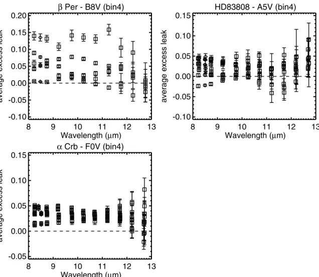
4. HD 83808, α Crb, and β Per (the triple system Algol) have clear signatures of companions in the excess leaks
measured (Figure2), showing very large fluctuations versus
hour angle, between 4% and 15% peak to peak. Given the uncertainties in the nuller off-axis transmission values and binary system parameters (companion position, diameter, and relative flux), the effect of these companions cannot be removed with high precision. As a result, these three stars are discarded from any further derivation of circumstellar dust excess and exozodi level (“bin 4” object type in
Table1).
The effective KIN exozodi sample is then reduced to 44 stars: 40 effectively single for KIN, one binary system with accurate dust excess determination (ι Peg), and three more binary systems for which only upper limits are derived (61 Cyg A, δ Tri, and β Tri).
3.4. 8–9 µm Excesses
As can be seen in all panels of Figure1, the excess
measure-ment uncertainty increases sharply with wavelength across the bandpass. The reason is that various instrumental factors (fi-nite diffraction effects, material absorption, and pinhole mode matching) and the increased thermal background strongly re-duce the KIN spectral sensitivity toward the red end of the bandpass. In addition, atmospheric dispersion is actively cor-rected around 9 µm, yielding larger chromatic effects and null
uncertainties at longer wavelengths (Colavita et al.2009). Under
these conditions, the most reliable excess estimates come from measurements obtained in the 8–9 µm bin. The quantity of in-terest is the ratio of the measured leak excess to its uncertainty, which we refer to hereafter as the “excess significance.” It is worth noting that as a result of instrumental noise, the measured leak excess can be negative, and the excess significance as well.
All excess measurements are summarized in Table2and show
that five stars have an 8–9 µm excess leak with a significance larger than 3σ . Among them, only η Crv shows a large (8σ ) excess. The other four are β UMa, β Leo, ζ Lep, and γ Oph, all showing excesses at the 3σ –4σ level. While 8–9 µm excesses
around η Crv and γ Oph were already reported inPaper I, KIN
excesses around the other three stars are reported here for the first time. Noticeably, all five stars had FIR excesses previously reported. A more detailed analysis of these five stars is given in
β Per - B8V (bin4)
8
9
10
11
12
13
Wavelength (µm)
-0.10
-0.05
0.00
0.05
0.10
0.15
0.20
average excess leak
HD83808 - A5V (bin4)
8
9
10
11
12
13
Wavelength (µm)
-0.10
-0.05
0.00
0.05
0.10
0.15
average excess leak
α Crb - F0V (bin4)
8
9
10
11
12
13
Wavelength (
µm)
-0.05
0.00
0.05
0.10
0.15
average excess leak
Figure 2. Excess leaks measured by the KIN for three stars with obvious signatures of stellar companions in the data (type “bin 4”). All available measurements
are displayed, showing large null fluctuations vs. time and baseline azimuth. These stars have been discarded from subsequent zodiacal dust level estimations and correspond to the last three targets listed in Table1.
3.5. Zodi Levels
In order to interpret the excess measurements and compare
them with the solar system case, we used the Zodipic code13to
create images of zodi clouds around each target. Zodipic syn-thesizes brightness distributions of exozodiacal clouds based on the empirical fits to the observations of the solar zodiacal cloud
made by COBE (Kelsall et al.1998). When Zodipic generates
a model brightness distribution for a zodi disk analog around a star other than the Sun, the dust has the same optical depth at 1 AU and the same radial density profile as in the solar system. As a convenient unit, we refer to this model as corresponding to 1 “zodi.” Zodipic scales the radial temperature profile with stellar luminosity, and the inner dust radius is set by a dust sub-limation temperature of 1500 K. The dust inner radius is thus dependent on stellar spectral type and ranges from 0.004 AU for the coolest star in our sample (the M2V star HIP 54035) to 0.18 AU for Vega. In the Zodipic code, the dust density can be treated as a free parameter, allowing generation of brightness distributions for a scaled version of the solar system (the total flux due to the circumstellar dust scales linearly with zodi level). Since the 8–9 µm KIN measurements are of higher quality, we restricted the zodi-level calculations to that spectral bin, which
13 http://ssc.spitzer.caltech.edu/dataanalysistools/tools/contributed/ general/zodipic/
also ensures continuity with the results derived inPaper I. In
or-der to convert the measured 8–9 µm excess leaks to number of
zodis, we used the procedure described in Section4.2ofPaper I,
summarized below. A one zodi dust cloud image (not including the central star) is generated around each star considered using the Zodipic model, and the overall dust flux transmitted through the instantaneous (8.5 µm) KIN transmission pattern (see
Appendix A) is computed. The resulting flux is then divided
by the 8.5 µm stellar flux, yielding the leak excess expected for a one zodi exozodical dust cloud, and a final estimate of the zodi level is required to match the observed excess leak. Since the dust cloud inclination and phase angle are generally unknown
(except in a few cases; see Section5.1), this operation is repeated
for different exozodiacal disk orientations, from face-on to
edge-on, with P.A. parallel and perpendicular14 to the
instan-taneous direction of the long-baseline fringes. These orienta-tion effects are small compared to the KIN excess measurement error bars, but they are included in all derived zodi levels and
uncertainties, which are listed in Table2. We note that, although
unphysical, negative zodis are allowed as a result of the error bars on the leak measurements. This procedure is exactly the
same as used inPaper I(Section4.2). We note, however, that in
14 Because of the finite scale height of the zodi dust cloud and the high spatial
resolution of the KIN, an edge on-disk still contributes a significant null excess whatever the baseline orientation.
Table 2
KIN Results Summary in the Context of Other IR Excess Measurements
Star E8–9 σ8–9 S8–9 Zodis E8–13 σ8uncor–13 Suncor σ8cor–13 Scor NIR/MIR/FIR Tcold
Excesses (K) ηCrv 2.7e-02 3.2e-03 8.35 1813 ± 209 4.4e-02 2.0e-03 22.30 5.1e-03 8.69 Na/Yb/Yc 50 βUMa 7.1e-03 1.8e-03 4.02 327 ± 80 6.4e-03 9.2e-04 7.00 2.5e-03 2.54 Na/Yb/Yc,x 140 βLeo 5.6e-03 1.4e-03 3.96 291 ± 73 4.2e-03 6.8e-04 6.17 1.9e-03 2.21 Ya/Yb/Yc,d 125 ζLep 5.9e-03 1.8e-03 3.30 243 ± 73 9.6e-03 1.2e-03 8.31 3.1e-03 3.12 Na/Yb/Ye 190 γOph 8.7e-03 2.8e-03 3.08 306 ± 99 1.1e-02 1.9e-03 5.96 5.1e-03 2.22 Na/Yf/Yf 80 Vega 2.1e-03 8.9e-04 2.30 297 ± 124 2.2e-03 3.4e-04 6.32 1.0e-03 2.13 Ya/Ye,g/Ye 90 ϵEri 2.5e-03 1.2e-03 2.16 262 ± 117 1.8e-03 5.0e-04 3.61 1.4e-03 1.26 Na/Yh/Yh 55
λAur 6.2e-03 3.0e-03 2.06 473 ± 226 5.6e-03 2.3e-03 2.40 6.2e-03 0.91 N/N/N
10 Tau 7.6e-03 4.1e-03 1.84 614 ± 333 2.4e-03 3.2e-03 0.76 8.8e-03 0.28 Ya/N/Yi 100 70 Vir 4.0e-03 2.2e-03 1.84 397 ± 208 5.6e-03 1.3e-03 4.30 3.5e-03 1.60 Na/Yj/Yk,l 65 61 Vir 5.1e-03 3.0e-03 1.70 381 ± 221 4.6e-03 2.5e-03 1.81 6.6e-03 0.69 N/Ni/Yi,m 70
ηCas A 3.1e-03 2.0e-03 1.55 267 ± 172 3.3e-03 9.9e-04 3.30 2.7e-03 1.21 Na/N/N Altair 2.1e-03 1.4e-03 1.50 247 ± 176 3.8e-03 5.1e-04 7.57 1.5e-03 2.55 Ya/Nn/No τBoo 3.1e-03 2.1e-03 1.46 208 ± 142 2.1e-03 1.7e-03 1.24 4.5e-03 0.47 N/Np/Nq 1 Ori 3.0e-03 2.1e-03 1.41 215 ± 151 1.7e-03 1.2e-03 1.38 3.4e-03 0.50 Na/N/N KX Lib 3.5e-03 2.5e-03 1.38 326 ± 235 −1.1e-03 1.9e-03 −0.58 4.9e-03 −0.23 N/N/N
βCom 5.8e-03 4.8e-03 1.20 389 ± 326 3.0e-03 2.2e-03 1.34 6.0e-03 0.50 N/N/N
αPsa 1.5e-03 1.4e-03 1.05 118 ± 107 3.7e-03 5.4e-04 6.96 1.6e-03 2.34 Yr/Ys/Yt 70 βCas 2.1e-03 2.0e-03 1.03 226 ± 216 1.7e-03 7.7e-04 2.24 2.2e-03 0.77 Na/N/Yu 120
ζAql 3.6e-03 4.4e-03 0.82 137 ± 167 1.8e-03 1.7e-03 1.04 5.0e-03 0.36 Ya/N/N
κCrb 3.5e-03 4.4e-03 0.80 625 ± 791 6.4e-03 2.2e-03 2.91 5.9e-03 1.08 Ya/N/Yv 60
ιPsc 2.4e-03 3.0e-03 0.79 183 ± 230 8.2e-03 1.7e-03 4.67 4.8e-03 1.71 N/N/N
107 Psc 2.0e-03 3.0e-03 0.67 160 ± 236 8.3e-03 2.5e-03 3.39 6.8e-03 1.23 Na/N/N 61 Cyg A∗ 1.3e-03 2.2e-03 0.60 127 ± 212 2.1e-03 1.0e-03 2.00 2.8e-03 0.74 Na/N/N 70 Oph A 1.2e-03 2.2e-03 0.56 136 ± 237 −1.1e-03 9.9e-04 −1.09 2.8e-03 −0.39 Na/N/N 47 UMa 1.4e-03 2.8e-03 0.50 105 ± 207 −1.8e-03 2.0e-03 −0.91 5.3e-03 −0.34 N/N/N αCep 3.4e-04 2.0e-03 0.17 24 ± 144 9.1e-04 9.7e-04 0.93 2.7e-03 0.34 Ya/N/N
δUMa −2.7e-04 2.4e-03 −0.11 −15 ± 140 3.8e-03 1.4e-03 2.81 3.7e-03 1.05 Na/Ye/ Ye 215 HIP 54035 −3.9e-04 2.5e-03 −0.16 −53 ± 366 −2.6e-03 2.0e-03 −1.35 5.2e-03 −0.50 N/N/N
ηLep −5.6e-04 1.7e-03 −0.32 −34 ± 113 −3.9e-03 1.1e-03 −3.62 2.8e-03 −1.37 Ya/Yp/Yl 170 υAnd −1.1e-03 3.1e-03 −0.34 −76 ± 226 −8.3e-04 1.9e-03 −0.43 5.2e-03 −0.16 Na/N/N
χ1Ori −9.2e-04 2.7e-03 −0.34 −60 ± 190 −8.2e-04 1.3e-03 −0.63 3.6e-03 −0.23 N/N/N
τCeti −1.1e-03 2.1e-03 −0.53 −95 ± 180 −8.4e-04 1.2e-03 −0.68 3.3e-03 −0.25 Ya/N/Yw 60 θPer −1.6e-03 2.8e-03 −0.56 −112 ± 204 3.7e-04 1.7e-03 0.22 4.5e-03 0.08 Na/N/N
ιPeg∗ −1.4e-03 2.5e-03 −0.57 −100 ± 173 −4.2e-03 1.2e-03 −3.38 3.4e-03 −1.24 N/N/N
βVir −2.1e-03 3.0e-03 −0.70 −170 ± 243 −3.7e-04 1.2e-03 −0.31 3.3e-03 −0.11 Na/N/N κ1Cet −3.6e-03 3.6e-03 −0.98 −249 ± 255 −8.5e-03 2.3e-03 −3.67 6.1e-03 −1.39 N/N/N
λGem −3.0e-03 3.0e-03 −1.00 −139 ± 140 −4.1e-03 2.3e-03 −1.80 6.1e-03 −0.67 Ya/N/N δ T ri∗ −3.7e-03 3.0e-03 −1.24 −298 ± 242 −6.6e-03 1.9e-03 −3.44 4.5e-03 −1.46 N/N/N
β T ri∗ −6.5e-03 4.7e-03 −1.39 −436 ± 316 −7.1e-04 2.4e-03 −0.30 6.2e-03 −0.11 N/N/Yo 90
NSV 4765 −4.6e-03 3.0e-03 −1.53 −477 ± 316 −3.1e-03 2.3e-03 −1.37 6.3e-03 −0.50 N/N/N γLep −3.0e-03 1.8e-03 −1.67 −205 ± 127 −1.1e-03 9.0e-04 −1.23 2.4e-03 −0.46 N/N/N ιPer −4.5e-03 2.5e-03 −1.82 −338 ± 188 −2.5e-04 1.4e-03 −0.18 3.7e-03 −0.07 N/N/N γSer −4.4e-03 2.3e-03 −1.87 −304 ± 164 −3.3e-03 1.3e-03 −2.47 3.7e-03 −0.90 Na/N/N
Notes. Column description. Star: targets observed by the KIN, sorted by decreasing excess significance in the 8–9 µm bin (S8−9).∗: targets with companions within KIN
FOV (see Section3.3); E8–9: 8–9 µm excess leak; σ8–9: 8–9 µm excess leak uncertainty; 8–9 µm excess significance S8−9= (E8−9/σ8−9); E8−13: 8–13 µm excess leak; σuncor
8−13: 8–13 µm excess leak uncertainty assuming uncorrelated spectral channels; Suncor= (E8−13/σ8−13uncor): 8–13 µm excess significance in the uncorrelated case; σcor
8−13: 8–13 µm excess leak uncertainty assuming fully correlated spectral channels; Scor= (E8−13/σ8−13cor ): 8–13 µm excess significance in the fully correlated case; “NIR/MIR/FIRµm excess” indicates whether a circumstellar excess has been reported in the NIR around 2.2 µm (a: Absil et al.2013), in the MIR (defined here
as “any wavelength between 15 and 35 µm”), or in the FIR (anywhere between 70 and 160 µm); Tcoldis the outer cold dust temperature derived from the MIR/FIR
excesses when available, assuming blackbody emission at a single radius.b: Chen et al. (2006),c: Matthews et al. (2010),d: Churcher et al. (2011),e: Su et al. (2006), f: Su et al. (2008),g: Su et al. (2013),h: Backman et al. (2009),i: Trilling et al. (2008),j: Bryden et al. (2009),k: Dodson-Robinson et al. (2011),l: Eiroa et al. (2013), m: Wyatt et al. (2012),n: Rieke et al. (2005),o: Gaspar et al. (2013),p: Lawler et al. (2009),q: Beichman et al. (2006b),r: Absil et al. (2009),s: Stapelfeldt et al.
(2004),t: Acke et al. (2012),u: Rhee et al. (2007),v: Bonsor et al. (2013),w: Habing et al. (2001),x: Booth et al. (2013).
this paper we have used more accurate estimates of the stellar flux in the KIN 8–9 µm spectral bin. We have used Akari fluxes in the 9 µm band, color corrected, and scaled to the 8.5 µm KIN effective wavelength using a Rayleigh–Jeans assumption. These revised stellar fluxes result in new estimates of the zodi levels
for the 25 stars ofPaper I, in average 40% higher, and supersede
those ofPaper I.
3.6. 8–13 µm Excesses
In addition to the 8–9 µm bin, we made use of the measure-ments obtained over the full N band, with the goal of iden-tifying possible new excess stars, i.e., stars with excess only present at the longest KIN wavelengths. To this end, we inter-preted each of the 10 spectral channel excess leaks as individual
measurements of a constant broadband 8–13 µm excess and formed an average. A difficulty in averaging such measurements is that some correlation is suspected between the different KIN
spectral channels (Colavita et al.2009), but that the actual
spec-tral data covariance matrix is unknown. In this case where the exact correlation pattern is unknown, a robust way of estimat-ing the mean is to ignore all correlation terms and use a simple
weighted average (Schmelling1995). Assuming that each
spec-tral channel (index k) is characterized by a measured excess leak
Ekwith 1σ Gaussian error σk, we then estimated the broadband
excess as E8−13= % kEk/σk2 % k1/σk2 . (8)
The uncertainty on this estimated broadband excess is more difficult to assess. In order to bound the problem, and since correlation factors are unknown, we examine two extreme cases.
3.6.1. Uncorrelated Spectral Channels
If all spectral channel measurements were completely uncor-related (the most optimistic scenario), the uncertainty on the broadband excess would be
σ8−13= , 1 % k1/σk2 . (9)
In this uncorrelated case, the broadband excess significance would then be given by
Suncor=E8−13 σ8−13 = % kEk/σk2 &% k1/σk2 . (10)
In particular, if all 10 spectral channels had the same
measure-ment uncertainty σk= σ0(a simple illustrative case to consider),
one would get
E8−13= ⟨Ek⟩, σ8−13= √σ0 10, Suncor=√10 ⟨ Ek⟩ σ0 . (11)
The broadband excess derived is simply the mean of observed values, and its significance increases as the square root of the number of spectral channels, as expected for uncorrelated data.
3.6.2. Fully Correlated Spectral Channels
Unfortunately, excess measurements obtained in different spectral channels are known to be partially correlated (Colavita
et al.2009), an effect believed to be caused by residual thermal
background correlation at the single telescope cross-combiner level and by small differential dispersion effects between science targets and calibrators. In order to derive the most conservative error bar on the broadband excess, we assume here that the various spectral channel measurements are fully correlated (worst-case scenario). In that case, the uncertainty on the broadband excess is given by
σ8−13= % k1/σk % k1/σk2 , (12)
and the broadband excess significance becomes
Scor= E8−13 σ8−13 = % kEk/σk2 % k1/σk . (13)
And if all 10 spectral channels had the same measurement
uncertainty σk= σ0, one would then get
E8−13= ⟨Ek⟩,
σ8−13= σ0,
Scor =⟨Ek⟩
σ0 . (14)
Compared to the uncorrelated case above, the uncertainty is now
higher by√10, and the broadband excess significance is reduced
by this factor. Table 2 summarizes the broadband 8–13 µm
excess leak measured for each star, with the uncertainties and significances derived in both the uncorrelated and fully correlated cases. The former is only given for reference (best-case scenario). Only the values derived in the fully correlated case (worst-case scenario) are considered for determining a potential 8–13 µm excess and for further statistical analysis.
3.6.3. 8–13 µm Excess Stars
Based on the results of Table2, and assuming that all spectral
channel measurements are fully correlated, only two stars show a broadband excess with a significance larger than 3σ : η CrV and ζ Lep. However, the statistical analysis conducted in the next section suggests that many more stars have a broadband excess, albeit close to the detection limit of the KIN.
4. STATISTICAL ANALYSES
Rather than looking at the results for individual stars, we use here the whole sample or specific subgroups of it. The goal is to obtain more sensitive estimates of the number of stars with a MIR excess and look for possible statistical trends, such as correlation of the observed KIN excesses with basic stellar properties. In order to avoid any possible contamination of the null measurements, all further analyses are limited to the 40
“effectively single” stars, as defined in Section3.3.
4.1. 8–9 µm Excess Distribution
Figure 3(a) shows the histogram of excess significance
measured in the 8–9 µm bin. As already discussed in Section3.3,
five stars show an excess significance greater than 3 and have hence a formally detected KIN excess. But as can be readily seen, the observed distribution tells more: it is highly nonsymmetrical and shows a tail toward larger excesses. Excess measurements with a “negative significance” are a consequence of the measurement noise, but this also means that such data can be used to infer the instrumental noise distribution. The dotted line shows the best Gaussian fit to these negative significance histogram data (after symmetrizing around x = 0 and taking into account the averaging due to finite bin size). The best-fit Gaussian noise distribution has a standard deviation of 1.002, very close to unity, as would be expected from the empirical standard deviation of many independent realizations of the
variable (E8−9/σE8−9). Further evidence for the validity of this
instrumental noise estimation and its Gaussianity is given in
Section4.5.15 Although they cannot be formally identified as
15 As shown in Figure4(a), which concentrates exclusively on the 20 stars
with no infrared excess previously known, a zero-mean Gaussian distribution with a standard deviation close to unity is also found to be a very good fit to the data (also seePaper I).
Figure 3. Statistical analysis. Histograms derived from the KIN measurements of 40 “effectively single” stars. (a) Histogram of the 8–9 µm excess significance. The
observed histogram is highly asymmetric and obviously skewed toward positive excesses, with five stars showing excesses detected at the >3σ level. (b) Histogram of exozodi levels (expressed in solar zodi units, 150 zodis per bin) derived from the KIN 8–9 µm measurements. The observed histogram is again asymmetric and obviously skewed toward zodi levels higher than the average measurement error of 200 zodis rms, showing a large number of measurements between 150 and 450 zodis. (c) Histogram of broadband 8–13 µm excess significance. Broadband excess error bars and significance are estimated assuming full correlation between the 10 spectral channels, which is the worst-case scenario. The observed histogram is also asymmetric with a tail extending toward positive excesses, two stars showing excesses detected at the >3σ level, and six more above 2σ . For each plot, the dashed line indicates for comparison the instrumental noise distribution derived from the data, assuming Gaussian behavior (see Sections4.1–4.3for details).
Figure 4. Comparing KIN results for stars with no infrared excesses previously known (top panels) and stars with cold (FIR) or hot (NIR) infrared excesses previously
detected (bottom panels). Each subgroup is composed of 20 stars. ((a) and (d)) Histograms of the measured 8–9 µm excess significance. ((b) and (e)) Histograms of exozodi levels derived from the 8–9 µm measurements, where each bin is 200 solar zodis wide. ((c) and (f)) Histograms of the measured 8–13 µm excess significance. ηCrv appears as a clear outlier in all lower panel histograms, with a high excess significance (>8) and the largest measured zodi level (1870 zodis). For all panels, the dashed lines indicate the best-fit Gaussian distribution to the data (ignoring η Crv for the lower panel fits). Stars with previously detected cold (FIR) or hot (NIR) excesses have observed distributions systematically shifted toward higher excess significance and zodi levels, with a high number of measurements concentrating between 200 and 400 solar zodis and three above 600 zodis (panel (e)). They are also the only stars to show 8–9 µm excesses detected above 3σ (five stars in panel (d)) or 8–13 µm excesses detected above 2σ (eight stars in panel (f)).
bona fide excess stars, there are several more targets with excess significance at the 1σ –3σ level than predicted by instrumental noise only: in addition to the five stars with significant excess, about 10 more stars lie close to the KIN detection limit and would be interesting targets for an instrument providing better contrast, even by just a factor of ≃3.
4.2. Exozodi Level Distribution
Figure 3(b) shows the histogram of zodi levels derived
around the 40 stars in the sample. Here again, the dotted line shows the best-fit Gaussian to the negative measurements, providing an estimate of the measurement noise distribution. Its standard deviation is 190 zodis, a value very close to the mean and median zodi measurement uncertainty of the overall sample (202 and 188 zodis, respectively). The zodi level and the excess significance are not necessarily related, since zodi level and uncertainty levels are a priori uncorrelated (e.g., a large zodi level might be associated with a large uncertainty and hence a low detection confidence level.) This means that the excess significance and zodi-level histograms provide independent information, at least to some extent. However, and quite interestingly, a similar behavior is found in the empirical histograms of both quantities. Once again, there seem to be significantly more than five stars with zodi levels higher than what the noise distribution predicts. This excess is particularly visible between 150 and 450 zodis.
4.3. Broadband Excess Distribution
Figure 3(c) shows the histogram of excess significance
measured between 8 and 13 µm, assuming that all spectral channels are fully correlated. This assumption yields the lowest possible excess significance levels given the data, and hence the most conservative estimates of broadband excess detection. While only two stars (η Crv and ζ Lep) show formally detected correlated broadband excesses with a significance greater than 3σ , the observed distribution is again very asymmetric, and the number of stars with significance between 1σ and 3σ again exceeds the levels predicted by pure instrumental noise. In addition, the best-fit noise distribution (dotted curve) derived from “negative excess” data has a standard deviation of 0.68. This low value suggests that the broadband excess significance estimates are generally underestimated by a factor of ≃1.5. In other words, any star with a correlated broadband excess quoted at the 2σ level is more likely a 3σ excess. Some further evidence for overestimated error bars comes from the analysis of the subsample of 20 stars with no infrared excess previously
known, presented in Section4.5.16Applying a 2σ cut instead of
3σ (per the argument presented above) leaves eight sources: the
five stars with 8–9 µm excess already listed in Section3.3(η
Crv, β UMa, β Leo, ζ Lep, and γ Oph), along with Fomalhaut (α Psa), Altair, and Vega.
4.4. Influence of Spectral Type and Age
Considering the 8–9 µm excess significance measured as a function of spectral type, KIN excesses at the 3σ level or higher are exclusively found around early-type stars. With the exception of η Crv (F2V type), all stars showing an 8–9 µm excess are A stars. Of course, the analysis suffers from small number statistics, but the observed fractions of excess stars
16 In this case, a zero mean Gaussian distribution with a standard deviation of
0.64—again notably smaller than unity—is found to be the best fit to the broadband excess significance histogram (Figure4(c)).
are very different at 4/11, 1/13, 0/9, and 0/7 for A, F, G,
and K/M17 stars, respectively. Extending the analysis to the
KIN broadband 8–13 µm measurements, A stars are even more favored: among the eight stars showing an excess significance at the 2σ level or higher, seven are A stars. This is in contrast with the results found for stars with no previously known infrared
excess (Paper I, Appendix A), for which no correlation was
found between excess leakage and stellar effective temperature. In fact, if any instrumental bias was affecting the measurements, it would rather tend to underestimate excesses around nearby A and early F stars. Indeed, while the KIN baseline is long enough to comfortably resolve the inner zodi regions of even the coldest and most distant stars in the sample, only nearby A and F stars
have 300 K dust radii lying outside of the KIN OWA (Table1).
As discussed before (Section3.2), this effect is precisely the
strongest around Vega, Altair, α Psa, β Leo, and β UMa. This suggests that the small excess leak detected around some of these stars could actually trace a significantly larger MIR physical
excess (see Section 5.2 for discussion of individual targets).
The higher occurrence of 10 µm excess observed around A stars appears then to be a real astrophysical trend. Since A stars have the shortest main-sequence lifetime, this apparent correlation of the KIN excess with spectral type could also be caused by a correlation with age. A similar trend was observed at FIR
and near-infrared (NIR) wavelengths (Trilling et al.2008; Absil
et al.2013).
4.5. Connection with Excesses Detected at Other IR Wavelengths
As summarized in Table 2 (last column), 20 of the KIN
“single” stars have either a “cold” FIR (>60 µm) excess or a “hot” NIR (≃2.2 µm) excess detected. While the former excess type is likely due to outer dust and comet reservoirs analogous to the solar system Kuiper Belt, the origin of the NIR excess is still poorly understood. The most likely explanation is the presence of submicron-sized hot dust particles piling up close to the
sublimation radius of these stars (Absil et al.2013; Mennesson
et al.2011; Lebreton et al.2013). In order to help understand the
origin of those various types of infrared excess, we correlated them with the detected KIN excess.
Figure4 compares the distribution measured for stars with
no previously known infrared excess (Group 1) with that obtained for stars with either a cold or a hot infrared excess previously reported (Group 2). Each group contains 20 stars each, allowing a straightforward comparison of the observed distributions. While distributions measured for the first group are centered around zero and fairly symmetric, the second-group distributions are heavily skewed toward positive detections. This effect is especially pronounced for the broadband KIN
measurements (Figure4, panels (c) and (f)). Indeed, while none
of the 20 stars in Group 1 show a large broadband excess significance (all below a value of 1.7), eight of the Group 2 stars show a broadband excess significance larger than 2. A similar effect is seen between the zodi-level distributions of the
two groups (Figure4, panels (b) and (e)): stars in Group 2 have
their observed distribution shifted toward higher zodi levels, exhibiting significantly more stars in the 200–400 zodi-level bin and at zodi levels above 600 zodis. Even after excluding η Crv and its unusually bright MIR dust emission, the weighted mean of the zodi levels measured for Group 2 stars is 206
17 There was only one M star in the sample (HIP 54035, M2V spectral type).