arXiv:1607.01035v1 [astro-ph.SR] 4 Jul 2016
DETECTION OF SOLAR-LIKE OSCILLATIONS, OBSERVATIONAL CONSTRAINTS, AND STELLAR MODELS FOR θ CYG, THE BRIGHTEST STAR OBSERVED BY THE KEPLER MISSION
J. A. Guzik1, G. Houdek2, W. J. Chaplin3,2, B. Smalley4, D. W. Kurtz5, R.L. Gilliland6, F. Mullally7, J.F. Rowe7, S. T. Bryson8, M. D. Still8,9, V. Antoci2, T. Appourchaux10, S. Basu11, T. R. Bedding12,2, O. Benomar12,13, R. A. Garcia14, D. Huber12,2, H. Kjeldsen2, D. W. Latham15, T.S. Metcalfe16, P. I. P´apics17, T. R.
White12,18,2, C. Aerts17,19, J. Ballot34, T. S. Boyajian11, M. Briquet20, H. Bruntt2,21, L. A. Buchhave22,23, T. L. Campante3,2, G. Catanzaro24, J. Christensen-Dalsgaard2, G. R. Davies3,2,14, G. Do˘gan2,26,27, D. Dragomir28, A. P.
Doyle25,4,Y. Elsworth3,2, A. Frasca24, P. Gaulme29, 30, M. Gruberbauer31, R. Handberg2, S. Hekker32,2, C. Karoff2,26, H. Lehmann33, P. Mathias34,35, S. Mathur16, A. Miglio3,2, J. Molenda- ˙Zakowicz36, B. Mosser37, S. J.
Murphy12,2, C. R´egulo38,39, V. Ripepi40, D. Salabert14, S. G. Sousa41, D. Stello12,2, K. Uytterhoeven38,39 1Los Alamos National Laboratory, XTD-NTA, MS T-082, Los Alamos, NM 87545 USA
2
Stellar Astrophysics Centre, Department of Physics and Astronomy, Aarhus University, Ny Munkegade 120, DK-8000 Aarhus C, Denmark 3School of Physics and Astronomy, University of Birmingham, Birmingham B15 2TT, UK
4
Astrophysics Group, School of Physical & Geographical Sciences, Lennard-Jones Laboratories, Keele University, Staffordshire, ST5 5BG, UK
5Jeremiah Horrocks Institute, University of Central Lancashire, Preston PR1 2HE, UK
6Center for Exoplanets and Habitable Worlds, The Pennsylvania State University, University Park, PA 16802 USA 7SETI Institute/NASA Ames Research Center, Moffett Field, CA 94035 USA
8
NASA Ames Research Center, Bldg. 244, MS-244-30, Moffett Field, CA 94035 USA 9Bay Area Environmental Research Institute, 560 Third Street W., Sonoma, CA 95476 USA 10
Institut d’Astrophysique Spatiale, Universit`e de Paris Sud–CNRS, Batiment 121, F-91405 ORSAY Cedex, France 11Department of Astronomy, Yale University, PO Box 208101, New Haven, CT 06520-8101 USA
12Sydney Institute for Astronomy (SIfA), School of Physics, University of Sydney, NSW 2006, Australia 13
NYUAD Institute, Center for Space Science, New York University Abu Dhabi, PO Box 129188, Abu Dhabi, UAE
14Laboratoire AIM, CEA/DRF – CNRS - Univ. Paris Diderot – IRFU/SAp, Centre de Saclay, 91191 Gif-sur-Yvette Cedex, France 15
Harvard-Smithsonian Center for Astrophysics, 60 Garden Street, Cambridge, MA 02138 USA 16Space Science Institute, 4750 Walnut Street, Suite 205, Boulder, CO 80301 USA
17Instituut voor Sterrenkunde, KU Leuven, Celestijnenlaan 200D, B-3001 Leuven, Belgium 18Australian Astronomical Observatory, PO Box 915, North Ryde, NSW 1670, Australia
19Department of Astrophysics/IMAPP, Radboud University Nijmegen, 6500 GL Nijmegen, The Netherlands 20
Institut d’Astrophysique et de G´eophysique, Universit´e de Li`ege, Quartier Agora, All´ee du 6 aoˆut 19C, B-4000, Li`ege, Belgium 21Aarhus Katedralskole, Skolegyde 1, DK-8000 Aarhus C, Denmark
22
Niels Bohr Institute, University of Copenhagen, DK-2100 Copenhagen, Denmark
23Centre for Star and Planet Formation, Natural History Museum of Denmark, University of Copenhagen, DK-1350 Copenhagen, Denmark 24INAF-Osservatorio Astrofisico di Catania, Via S.Sofia 78, I-95123 Catania, Italy
25Department of Physics, University of Warwick, Gibbet Hill Road, Coventry CV4 7AL, UK
26Department of Geoscience, Aarhus University, Hoegh-Guldbergs Gade 2, DK-8000, Aarhus C, Denmark 27
High Altitude Observatory, National Center for Atmospheric Research, PO Box 3000, Boulder, CO 80307, USA 28The Department of Astronomy and Astrophysics, University of Chicago, 5640 S Ellis Ave, Chicago, IL 60637, USA 29Apache Point Observatory, Sloan Digital Sky Survey, PO Box 59, Sunspot, NM 88349, USA
30New Mexico State University, Department of Astronomy, PO Box 30001, Las Cruces, NM 88003-4500, USA
31Institute for Computational Astrophysics, Department of Astronomy and Physics, Saint Mary’s University, Halifax, NS B3H 3C3, Canada 32Max Planck Institute for Solar System Research, SAGE research group, Justus-von-Liebig-Weg 3, 37077 Gttingen, Germany
33Th¨uringer Landessternwarte Tautenburg (TLS), Sternwarte 5, D-07778 Tautenburg, Germany 34
Universit´e de Toulouse, UPS-OMP, IRAP, 65000, Tarbes, France 35CNRS, IRAP, 57 avenue d’Azereix, BP 826, 65008, Tarbes, France 36
Instytut Astronomiczny Uniwersytetu Wroc lawskiego, ul. Kopernika 11, 51-622 Wroc law, Poland
38Instituto de Astrof´ısica de Canarias, 38205, La Laguna, Tenerife, Spain 39Universidad de La Laguna, Dpto de Astrof´ısica, 38206, Tenerife, Spain
40INAF-Osservatorio Astronomico di Capodimonte, Via Moiariello 16, I-80131 Napoli, Italy 41
Instituto de Astrof´ısica e Ciˆencias do Espa¸co, Universidade do Porto, CAUP, Rua das Estrelas, 4150-762 Porto, Portugal ABSTRACT
θ Cygni is an F3 spectral-type main-sequence star with visual magnitude V=4.48. This star was the brightest star observed by the original Kepler spacecraft mission. Short-cadence (58.8 s) photometric data using a custom aperture were obtained during Quarter 6 (June-September 2010) and subsequently in Quarters 8 and 12-17. We present analyses of the solar-like oscillations based on Q6 and Q8 data, identifying angular degree l = 0, 1, and 2 oscillations in the range 1000-2700 µHz, with a large frequency separation of 83.9 ± 0.4 µHz, and frequency with maximum amplitude νmax = 1829 ± 54 µHz. We also present analyses of new ground-based spectroscopic observations, which, when combined with angular diameter measurements from interferometry and Hipparcos parallax, give Teff = 6697 ± 78 K, radius 1.49 ± 0.03 R⊙, [Fe/H] = -0.02 ± 0.06 dex, log g = 4.23 ± 0.03. We calculate stellar models matching the constraints using several methods, including using the Yale Rotating Evolution Code and the Asteroseismic Modeling Portal. The best-fit models have masses 1.35–1.39 M⊙and ages 1.0–1.6 Gyr. θ Cyg’s Teff and log g place it cooler than the red edge of the γ Doradus instability region established from pre-Kepler ground-based observations, but just at the red edge derived from pulsation modeling. The best-fitting models have envelope convection-zone base temperature of ∼320,000 to 395,000 K. The pulsation models show γ Dor gravity-mode pulsations driven by the convective-blocking mechanism, with periods of 0.3 to 1 day (frequencies 11 to 33 µHz). However, gravity modes were not detected in the Kepler data; one signal at 1.776 c d−1 (20.56 µHz) may be attributable to a faint, possibly background, binary. Asteroseismic studies of θ Cyg, in conjunction with those for other A-F stars observed by Kepler and CoRoT, will help to improve stellar model physics to sort out the confusing relationship between δ Sct and γ Dor pulsations and their hybrids, and to test pulsation driving mechanisms.
Keywords: stars: interiors–stars: oscillations–asteroseismology–stars: θ Cyg 1. INTRODUCTION
The mission of the NASA Kepler spacecraft, launched 2009 March 7, was to search for Earth-sized planets around Sun-like stars in a fixed field of view in the Cygnus-Lyra region using high-precision CCD photom-etry to detect planetary transits (Borucki et al. 2010). As a secondary mission Kepler surveyed and monitored over 10,000 stars for asteroseismology, using the intrin-sic brightness variations caused by pulsations to infer the star’s mass, age, and interior structure (Gilliland et al. 2010a). After the failure of the second of four reac-tion wheels, the Kepler mission transireac-tioned into a new phase, K2 (Howell et al. 2014), observing fields near the ecliptic plane for about 90 days each, with a variety of science objectives including planet searches.
The V = 4.48 F3 spectral-type main-sequence star θ Cyg, also known as 13 Cyg, HR 7469, HD 185395, 2MASS 19362654+5013155, HIP 96441, and KIC 11918630, where KIC = Kepler Input Catalog (Brown et al. 2011), is the brightest star that fell on active pixels in the original Kepler field of view. θ Cyg is nearby and bright, so that high-precision ground-based data can be combined with high signal-to-noise and long time-series Kepler photometry to provide constraints
for asteroseismology. The position of θ Cyg in the HR diagram is near that of known γ Dor pulsators, suggesting the possibility that it may exhibit high-order gravity mode pulsations, which would probe the stellar interior just outside its convective core. θ Cyg is also cool enough to exhibit solar-like p-mode (acoustic) oscillations, which probe both the interior and envelope structure.
θ Cyg has been observed using adaptive optics (Desort et al. 2009). It has a resolved binary M-dwarf companion of ∼0.35 M⊙ with separation 46 AU. Follow-ing the orbit for nearly an orbital period (unfortunately ∼ 230 y) will eventually give an accurate dynamical mass for θ Cyg. Also, the system shows a 150-d quasi-period in radial velocity, suggesting that one or more planets could accompany the stars (Desort et al. 2009). θ Cyg has also been observed using optical interferom-etry (Ligi et al. 2012;Boyajian et al. 2012;White et al. 2013, see Section 4). These observations provide tight constraints on the radius of θ Cyg and therefore a very useful constraint for asteroseismology.
θ Cyg’s projected rotational velocity is low; v sin i = 3.4 ± 0.4 km s−1 (Gray 1984, see Section 3). If sin i is not too small, θ Cyg’s slow rotation should simplify
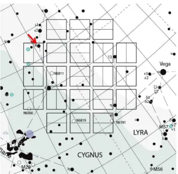
Figure 1. Kepler field of view with stars marked accord-ing to stellar magnitude created usaccord-ing “The Sky” astron-omy software (http://www.bisque.com/sc/pages/TheSkyX-Editions.aspx). The location of θ Cyg is shown by the red arrow, and is marked with the symbol θ and a filled circle designating magnitude 4-5. Note that all stars brighter than θ Cyg fall in the regions between the CCD arrays to avoid saturating pixels.
mode identification and pulsation modeling, as spherical approximations and low-order perturbation theory for the rotational splitting should be adequate.
This paper is intended to provide background on the θ Cyg system and to be a first look at the Kepler pho-tometry data and consequences for stellar models and asteroseismology. We present light curves and detection of the solar-like p-modes based on Kepler data taken in observing Quarters 6 and 8 (Section2). We summarize ground-based observational constraints from the litera-ture (Appendix A) and present analyses based on new spectroscopic observations (Section3) and optical inter-ferometry (Section 4). We discuss inference of stellar parameters based on the large separation and frequency of maximum amplitude (Section 5), line widths (Sec-tion6), and mode identification (Section7). We use the observed p-mode oscillation frequencies and mode iden-tifications as constraints for stellar models using several methods (Section8). We discuss predictions for γ Dor g-mode pulsations (Section 9), and results of a search for low frequencies consistent with g modes (Section 10). We conclude with motivation for continued study of θ Cyg (Section11).
We do not include in this paper the analyses of data from Quarters 12-17 for several reasons. First, we com-pleted the bulk of this paper, including the spectroscopic analyses, and first asteroseismic analyses at the time
when only the Q6 and Q8 data were available. Sec-ond, a problem has emerged with the Kepler data reduc-tion pipeline for the latest data release for short-cadence data1that will not be corrected until later in 2016; while
θ Cyg is not on the list of affected stars, because θ Cyg required so many pixels and special processing, more work is needed to confirm that the problem has not in-troduced additional noise in the light curve. We esti-mate that inclusion of the full time-series data will re-sult in finding a few more frequencies, and will improve the precision of the frequencies obtained by a factor of ∼1.8. Comparison of studies of the bright (V = 5.98) Keplertargets 16 Cyg A and B using one month versus thirty months of data show that the longer time series improved the accuracy and precision of results, but did not significantly change the frequencies or inferred stel-lar model parameters (Metcalfe et al. 2012,2015).
Detailed analyses making use of the remaining time-series data and the Kepler pixel data will be the subject of future papers.
2. DETECTION OF θ CYG SOLAR-LIKE OSCILLATIONS BY KEPLER
θ Cyg is seven magnitudes brighter than the satura-tion limit of the Kepler photometry. Figure1shows the Keplerfield of view superimposed on the constellations Cygnus and Lyra with θ Cyg on the CCD module at the top of the leftmost column in this figure. Kepler stars are observed using masks that define the pixels to be stored for that star. Special apertures can be de-fined to better conform to the distribution of charge for extremely saturated targets (see, e.g., Kolenberg et al. 2011). For θ Cyg the number of recorded pixels required was reduced from >10,000 to ∼1,800 by using an im-proved special aperture.
θ Cyg was observed 2010 June−September (Kepler Quarter 6) and 2011 Jan−March (Quarter 8) in short ca-dence (58.8 s integration; seeGilliland et al.(2010b) for details). Kepler measurements were organized in quar-ters because the satellite performed a roll every three months to maintain the solar panels directed towards the Sun and the radiators to cool the focal plane in shadow. Moreover, every month the satellite stopped data acqui-sition for less than 24 hours and pointed towards the Earth to transmit the stored data. Therefore, monthly interruptions occured in the Kepler observations. More details on the Kepler window function can be found in
Garc´ıa et al.(2014a).
Figure2shows the 90-day minimally processed short-cadence light curves for Q6 and Q8. θ Cyg was not well-captured by the dedicated mask for ∼50% of Quarter 6
1
(a problem resolved for observations in subsequent quar-ters), so 42 d of the best-quality data in the flat portion of the Q6 light curve were used in the pulsation analysis. During Q8, the spacecraft entered a safe mode Dec. 22-Jan. 6, causing data loss at the beginning of the quarter, so only 67 d of data were obtained.
These light curves were processed following the meth-ods described by Garc´ıa et al. (2011) to remove out-liers, jumps and drifts, as was done for other solar-like stars (e.g. Campante et al. 2011; Mathur et al. 2011a;
Appourchaux et al. 2012b), including the binary system 16 Cyg (Metcalfe et al. 2012), where a special treatment was also applied because it is composed of two very bright stars. For the solar-like oscillation analysis of θ Cyg, we have removed the drifts by using a triangular smoothing filter with a width of 10 days (frequency 1.16 µHz). The triangular smoothing filter is a rectangular (box car) filter of 10 days applied twice to the data; hence it is the convolution of two box cars, which is a triangle. Figure3shows the resultant light curve for the Q6 and Q8 data.
The Fourier Transform of the Q6 data revealed a rich spectrum of overtones of solar-like oscillations, with excess power above the background in the fre-quency range ∼1200 to 2500 µHz. Figure 4 shows the power-density spectrum of the processed Q6 and Q8 data. The data show a large frequency separation ∆ν of ∼84 µHz with maximum oscillation amplitude at νmax = 1830 µHz. The appearance of the oscil-lation spectrum is very similar to that of other well-studied F stars such as Procyon A (Bedding et al. 2010b;
Bond et al. 2015), HD49933 (Appourchaux et al. 2008;
Benomar et al. 2009b; Reese et al. 2012), HD181420 (Barban et al. 2009), and HD181906 (Garc´ıa et al. 2009); see also Table 1 ofMosser et al.(2013) and refer-ences therein. The envelope of oscillation power is very wide, and modes are evidently heavily damped, meaning the resonant peaks have large widths in the frequency spectrum, which makes mode identification difficult (see, e.g.,Bedding & Kjeldsen 2010a, and discussion in Sec-tion 7). For comparison to θ Cyg’s νmax (1830 µHz), the maximum in the Sun’s power spectrum is at about 3150 µHz, while for Procyon with mass 1.48 M⊙and lu-minosity 6.93 L⊙, νmaxis 1014 µHz (Huber et al. 2011), and for HD49933, with mass 1.30 M⊙ and luminosity 3.47 L⊙, νmaxis 1760 µHz (Appourchaux et al. 2008).
3. NEW HIGH-RESOLUTION SPECTRA AND ANALYSES
A review of the extensive literature prior to the Ke-pler observations suggests that θ Cyg is a normal, slowly rotating, solar-composition, F3V spectral-type star (Gray et al. 2003) with Teffaround 6700±100 K and log g around 4.3±0.1 dex (see Appendix A). This section
summarizes analyses of high-resolution spectra taken subsequent to the Kepler observations by P. I. P´apics at the HERMES spectrograph2 on the Mercator
Tele-scope3 in May 2011, and by the team of D. Latham at
the TRES spectrograph in December 2011. 3.1. HERMES spectrum analyses of θ Cygni High-resolution high signal-to-noise spectra were taken using the HERMES spectrograph (Raskin et al. 2011) installed on the 1.2-meter Mercator telescope based at the Roque de los Muchachos Observatory on La Palma, Canary Islands, Spain. The spectro-graph is bench-mounted and fiber-fed, and resides in a temperature-controlled enclosure to guarantee instru-mental stability. During the observations, HERMES was set to the HRF mode using the high-resolution fiber with a spectral resolving power of R = 85, 000 delivering a spectral coverage from 377 to 900 nm in a single expo-sure and a peak efficiency of 28%. The final processed orders, along with merged spectra, were obtained on site using the integrated HERMES data reduction pipeline. Analyses of the HERMES spectrum (Fig.5), discussed next, was undertaken independently by five of us, using differing methods.
3.1.1. vwa
The Versatile Wavelength Analysis (vwa) method uses spectral synthesis to fit lines to determine their equivalent widths (EWs). Teff is found by adjusting it to remove any slope in the Fe i versus excitation potential of the lower level, using lines with EW<100m˚A. The cri-terion for log g is that the average abundance from the Fe i and Fe ii lines agree. In addition, checks are made that Mg i b and Ca lines at 6122˚A and 6162˚A are well fitted. Since Van der Waals broadening is important for these lines, they have been adjusted to agree with the solar spectrum for log g = 4.437 (Bruntt et al. 2010b). The Fe abundance relative to solar, [Fe/H], is calculated as the mean of Fe i lines with EW<100 m˚A and >5 m˚A. Microturbulence, vmic, is found by minimizing Fe i abun-dances versus EW, using only lines with EW<90 m˚A. Model atmospheres are an interpolation in the MARCS grid, with line lists from VALD (Kupka et al. 1999). Us-ing a solar spectrum, each line has been forced to give the abundance inGrevesse et al.(2007), in order to give
2 Supported by the Fund for Scientific Research of Flanders (FWO), Belgium, the Research Council of KU Leuven, gium, the Fonds National Recherches Scientific (FNRS), Bel-gium, the Royal Observatory of BelBel-gium, the Observatoire de Gen`eve, Switzerland and the Th¨uringer Landessternwarte Taut-enburg, Germany
3
Operated on the island of La Palma by the Flemish Commu-nity, at the Spanish Observatorio del Roque de los Muchachos of the Instituto de Astrof´ısica de Canarias
Figure 2. Kepler θ Cyg unprocessed light curve for Quarter 6 (left) and Quarter 8 (right). The custom aperture captured the target completely in Q6 only during 42 d (flat portion of curve) used in this analysis. The spacecraft entered a safe mode for part of Q8, so only 67 days of data were obtained.
Figure 3. Combined Q6 and Q8 light curve after detrend-ing and applydetrend-ing a 10-day triangular filter to remove low-frequency variations.
the correction to the log gf values. Non-LTE effects are considered using Rentzsch-Holm(1996), since these ef-fects can be important for stars with Teff above 6500 K.
3.1.2. uclsyn
The analysis was performed based on the meth-ods given in Doyle et al. (2013). The uclsyn code (Smith & Dworetsky 1988;Smith 1992) was used to per-form the analysis and Kurucz atlas9 models with no overshooting were used (Castelli et al. 1997). The line list was compiled using the VALD database. The Hα and Hβ lines were used to give an initial estimate of Teff. The log g was determined from the Ca i line at 6439˚A, along with the Na i D lines. Additional Teff and log g diagnostics were performed using the Fe lines; however,
the Teff acquired from the excitation balance of the Fe i lines was found to be too high (∼ 6900 K) and this Teff was not used. A null dependence between the abun-dance and the equivalent width was used to constrain the microturbulence. The log g from the Fe lines was determined by requiring that the Fe i and Fe ii abun-dances agree, and the Teff was also determined from the ionization balance.
The quoted error estimates include that given by the uncertainties in Teff, log g, and vmic, as well as the scat-ter due to measurement and atomic data uncertainties. The projected stellar rotation velocity (v sin i) was de-termined by fitting the profiles of several unblended Fe i lines in the wavelength range 6000–6200˚A. A value for macroturbulence of 6 km s−1 was assumed, based on slight extrapolations of the calibration by Bruntt et al.
(2010a) andDoyle et al.(2014), and a best-fitting value of v sin i = 4.0 ± 0.4 km s−1was obtained.
3.1.3. rotfit
The rotfit method is based on a χ2 minimization with a grid of spectra of real stars with well-known astro-physical parameters (Frasca et al. 2006; Metcalfe et al. 2010;Molenda- ˙Zakowicz et al. 2013). Thus, full spectral regions (discarding those ones heavily affected by tel-luric lines), not individual lines, are used. The method derives Teff, log g, [Fe/H], v sin i and MK classification.
3.1.4. SynthV
Stellar parameters (Teff, log g, [M/H], vmic and v sin i) are obtained by computing synthetic spec-tra and comparing them to the observed spectrum (Lehmann et al. 2011). Atmosphere models were
calcu-Figure 4. Top: Power-density spectrum of the Q6 and Q8 data shown using the minimally processed data (grey) and using a box-car smoothing of width 3 µHz (black). Middle: Power spectrum with a smoothing of width 3 µHz (grey) or ∆ν/2 = 42 µHz (black). Superimposed is shown the best fit of the mode envelope with a Gaussian (red) and of the noise background (blue). Bottom: Zoom-in on the modes. The power spectrum is smoothed over 0.5 µHz (grey) or 3 µHz (black). The red curve shows the best fit to the individual pulsation modes with Lorentzian profiles.
lated with LLmodels (Shulyak et al. 2004), the com-putation of synthetic spectra was performed using Syn-thV (Tsymbal 1996). Atomic data were taken from VALD. The spectrum synthesis was done on the wave-length range 4047–6849 ˚A, covering both metal and the first four lines of the Balmer series. The local contin-uum of the observed spectrum was corrected to fit those of the synthetic ones. χ2 statistics were used to deter-mine the optimum values of the atmospheric parameters and their errors based on the 1-σ confidence space in all parameters.
3.1.5. ares+ moog
The stellar parameters were obtained from the auto-matic measurement of the equivalent widths of Fe i and Fe ii lines with ares (Sousa et al. 2007) and then im-posing excitation and ionization equilibrium using the moogLTE line analysis code (Sneden 1973) and a grid
of Kurucz atlas9 model atmospheres (Kurucz 1993). The Fe i and Fe ii line list comprises more than 300 lines that were individually tested using high-resolution spec-tra to check its stability to automatic measurement with ares. The atomic data were obtained from VALD, but with log gf adjusted through an inverse analysis of the Solar spectrum, in order to allow for differential abun-dance analyses relative to the Sun (Sousa et al. 2008). The errors on the stellar parameters are obtained by quadratically adding 100 K, 0.13 and 0.06 dex to the internal errors on Teff, log g and [Fe/H], respectively. These values were obtained by considering the typical dispersion plotted in each comparison of parameters pre-sented inSousa et al.(2008). A more detailed discussion on the errors derived for this spectroscopic method can be found inSousa et al.(2011).
Figure 5. High-resolution spectrum of θ Cyg taken with HERMES Mercator spectrograph in May 2011 (top), and region around Hγ (middle) and Hβ (bottom).
Two spectra were obtained with the Tillinghast Re-flector ´Echelle Spectrograph (TRES) on the 1.5-m Till-inghast Reflector at the Smithsonian’s Fred L. Whipple Observatory on Mount Hopkins, Arizona. The resolv-ing power of these spectra is 44,000, and the signal-to-noise ratio per resolution element is 280 and 351 for one-minute exposures on BJD 2455905.568 and 2455906.544, respectively. The wavelength coverage extends from 385 to 909 nm, but only the three orders from 506 to 531 nm were used for the analysis of the stellar parameters using Stellar Parameter Classification (SPC, Buchhave et al. 2012), a tool for comparing an observed spectrum with a library of synthetic spectra. spc is designed to solve simultaneously for Teff, [M/H], log g and v sin i. In essence, spc cross-correlates an observed spectrum with a library of synthetic spectra for a grid of Kurucz model atmospheres and finds the stellar parameters by deter-mining the extreme of a multi-dimensional surface fit to the peak correlation values from the grid.
The consistency between the spc results for the two observations was excellent, but undoubtedly the system-atic errors are much larger, such as the systemsystem-atic errors due to the library of synthetic spectra. Based on past experience, we assign floor errors of 50 K, 0.1 dex, 0.08 dex and 0.5 km s−1 for Teff, log g, [M/H] and v sin i, re-spectively. The library spectra were calculated assuming vmic= 2 km s−1. In tests of spc it has been noticed that the log g values can disagree systematically with cases that have independent dynamical determinations of the gravity for effective temperatures near 6500 K and above
Figure 6. A spectrum of θ Cyg in the order containing the Mg b triplet, obtained with the TRES spectrograph on the 1.5-m reflector at the Fred Lawrence Whipple Observatory on Mount Hopkins, Arizona. The resolving power is 44,000 and the SNR is 350 per resolution element of 6.8 km/s, at the center of the order. The exposure time was 60 seconds. The ´echelle blaze function has been removed by dividing with an exposure of a quartz iodine tungsten filament lamp.
(e.g., for Procyon and Sirius). Therefore, as discussed in the next section, we have also used spc to determine Teff and [M/H] whilst fixing log g to the value obtained from asteroseismology.
3.3. Stellar Parameters
A summary of the results from the spectral analyses is given in Table1. There is a relatively large spread in the values of Teff and log g obtained from the spectral anal-yses. Examination of their locations in the Teff–log g di-agram (Fig.7), shows an apparent correlation between these two parameters. This coupling between the two parameters is a known and common problem with spec-tral analyses, with some methods more susceptible than others.
To address this degeneracy, the spectral analyses were, therefore, repeated using a fixed log g = 4.23 ± 0.03 derived from the interferometric and asteroseismic con-straints on θ Cyg’s mass and radius fromWhite et al.
(2013), and which is also in line with the log g values of the best-fit asteroseismic models discussed in Section
8. The exception is rotfit, which due to its design for use with a grid of real stars, cannot be used to de-rive parameters for a fixed log g. The results from the other methods are presented in the lower part of Ta-ble1. With the exception of ares + moog, the model-atmosphere spectroscopic methods all agree to within the error bars and differ by less than 70 K. The ares + moogmethod is differential to the Sun, with a line list specifically prepared for precise analysis of stars with temperatures closer to solar, and, therefore, θ Cyg is too hot for this differential analysis.
It is interesting to explore why the model-independent rotfit method is giving slightly lower values.
Fit-Table 1. Summary of the results from the spectral analyses
vwa uclsyn rotfit SynthV ares+ moog spc
Teff (K) 6650 ± 80 6800 ± 108 6500 ± 150 6720 ± 70 6942 ± 106 6637 ± 50
log g 4.22 ± 0.08 4.35 ± 0.08 4.00 ± 0.15 4.28 ± 0.19 4.58 ± 0.14 4.11 ± 0.1
[Fe/H] −0.07 ± 0.07 +0.02 ± 0.08 −0.2 ± 0.1 −0.22 ± 0.05 0.08 ± 0.06 −0.07 ± 0.08
vmic(km s−1) 1.66 ± 0.06 1.48 ± 0.08 n/a 1.93 ± 0.25 1.94 ± 0.10 (2.0) †
v sin i (km s−1) n/a 4.0 ± 0.4 4.0 ± 1.5 6.36 ± 0.61 n/a 7.0 ± 0.5
fixing log g = 4.23 ± 0.03
Teff (K) 6650 ± 80 6715 ± 92 n/a 6716 ± 67 6866 ± 125 6705 ± 50
[Fe/H] −0.07 ± 0.07 −0.03 ± 0.09 n/a −0.21 ± 0.05 0.06 ± 0.06 −0.03 ± 0.08
vmic(km s−1) 1.66 ± 0.06 1.48 ± 0.08 n/a 1.92 ± 0.24 1.89 ± 0.10 (2.0) †
Note—† indicates an assumed value
3.8
4
4.2
4.4
4.6
4.8
6400
6500
6600
6700
6800
6900
7000
log
g
T
eff[K]
IRFM
3.8
4
4.2
4.4
4.6
4.8
6400
6500
6600
6700
6800
6900
7000
log
g
T
eff[K]
Direct
3.8
4
4.2
4.4
4.6
4.8
6400
6500
6600
6700
6800
6900
7000
log
g
T
eff[K]
3.8
4
4.2
4.4
4.6
4.8
6400
6500
6600
6700
6800
6900
7000
log
g
T
eff[K]
Literature
3.8
4
4.2
4.4
4.6
4.8
6400
6500
6600
6700
6800
6900
7000
log
g
T
eff[K]
VWA
ARES+MOOG
SynthV
ROTFIT
UCLSYN
SPC
Figure 7. Comparisons of results from the analyses of HERMES and TRES spectra. The range of values of Teff obtained by
Blackwell & Lynas-Gray(1998) using the IRFM is shown by the light grey band. The interferometric TefffromLigi et al.(2012)
and the asteroseismic log g value are given as the dark grey box labelled ‘Direct’. The dashed box indicates the most-probable parameters from the literature review.
ting a spectrum to a grid of empirical spectra of stars with known properties ought to give reliable results. The surface gravity is higher than what would ap-pear reasonable from external sources, including the measured stellar luminosity. Inspection of figure 4 in
Molenda- ˙Zakowicz et al. (2011) shows a similar differ-ence at high Teff: cooler Teff and lower log g compared to model atmosphere results by ∼200 K and ∼0.2 dex, respectively. In fact, applying those corrections would bring the rotfit results into better agreement with the other spectroscopic results.
From the remaining four spectral analyses, we obtain an average (after fixing log g) of Teff = 6697 ± 78 K, where the error has been determined from quadra-ture sum of the standard deviation of the average (31 K) and average of the individual methods’ er-rors (72 K). The latter is taken as a measure of the systematic uncertainty in the temperature deter-minations (G´omez Maqueo Chew et al. 2013). The re-sult is consistent with Teff = 6672 ± 47 K from the IRFM (Blackwell & Lynas-Gray 1998), and with Teff = 6767 ± 87 K (Ligi et al. 2012) or Teff = 6749 ± 44 K (White et al. 2013) from interferometry.
3.3.1. Metallicity
The values for metallicity obtained from the spectro-scopic analyses exhibit a scatter of nearly 0.3 dex. In order to compare these we need to ensure that they are all obtained relative to the same adopted solar value. The vwa and ares + moog methods are differen-tial with respect to the Sun and provide a direct de-termination of [Fe/H]. The uclsyn and spc analyses adopt theAsplund et al.(2009) solar value of log A(Fe) = 7.50, while the SynthV analysis uses log A(Fe) = 7.45 (Grevesse et al. 2007). Adopting theAsplund et al.
(2009) solar Fe abundance would decrease the SynthV value to [Fe/H] = −0.26. While this value is discrepant from the other analyses, it does agree with that found by rotfit using empirical spectra. The average metal-licity from all the spectroscopic analyses, with the fixed log g, is [Fe/H] = −0.07 ± 0.12 dex. If the SynthV analysis is omitted, then the value becomes [Fe/H] = −0.02 ± 0.06 dex. Thus we conclude that θ Cyg has a metallicity close to solar.
3.3.2. Rotational Velocity
The projected stellar rotational velocity (v sin i) was determined by four of the methods. The uclsyn anal-ysis assumed a macroturbulence of 6 km s−1 based on slight extrapolations of the calibrations byBruntt et al.
(2010a) andDoyle et al.(2014), while the SynthV and spc analyses set macroturbulence to zero. The rot-fit method which uses spectra of real stars implicitly includes macroturbulence and agrees with the result of
uclsyn. Setting macroturbulence to zero in the uclsyn analysis yields 6.4 ± 0.2 km s−1, which is in agreement with SynthV and spc. However, setting macroturbu-lence to zero is not a good assumption for slowly rotat-ing stars, and leads to a large overestimation of v sin i (seeMurphy et al. 2016, and references therein). Using Fourier techniques,Gray(1984) obtained v sin i = 3.4 ± 0.4 km s−1 and a macroturbulent velocity of 6.9 ± 0.3 km s−1. Given that we have not determined macrotur-bulence in our spectral analyses, we adopt Gray’s values.
4. INTERFEROMETRIC RADIUS
θ Cyg has also been the object of optical interferome-try observations. van Belle et al. (2008) used the Palo-mar Testbed Interferometer to identify 350 stars, in-cluding θ Cyg, that are suitably pointlike to be used as calibrators for optical long-baseline interferometric observations. They then used spectral energy distri-bution (SED) fitting (not the interferometry measure-ments) based on 91 photometric observations of θ Cyg to derive a bolometric flux at the stellar surface and a bolometric luminosity, and estimate its angular diame-ter to be 0.760 ± 0.021 milliarcsecond (mas). Combining this angular diameter estimate with the distance of 18.33 ± 0.05 pc given by the revised Hipparcos parallax 54.54 ± 0.15 mas (van Leeuwen 2007b), the derived radius of θ Cyg is 1.50 ± 0.04 R⊙.
Ligi et al. (2012) use observations from the VEGA/CHARA array to derive a limb-darkened angular diameter of 0.760 ± 0.003 mas, and a radius of 1.503 ± 0.007 R⊙. White et al.(2013) use data from the Precision Astronomical Visual Observations (PAVO) combiner and the Michigan Infrared Combiner (MIRC) at the CHARA array, to derive a limb-darkened angular diameter of 0.753 ± 0.009 mas, and a radius of 1.48 ± 0.02 R⊙. A radius of 1.49 ± 0.03R⊙ encompasses both theLigi et al.(2012) andWhite et al.(2013) values.
Interferometry has the potential to constrain the ra-dius of θ Cyg more accurately than spectroscopy and photometry alone. It is notable that all three results, thevan Belle et al.(2008) estimate, and those reported in the two later observational papers, agree within their error bars on the angular diameter of θ Cyg, and that the inferred radius is constrained to better than would be obtainable without the interferometric observations. If one were to use only the literature log L/L⊙ = 0.63 ± 0.03 (van Belle et al. 2008) (L = 4.26 ± 0.30L⊙) and Teff 6745 ±150K(Erspamer & North 2003) and their as-sociated error estimates to calculate the stellar radius, the derived radius would be 1.53 ± 0.13 R⊙.
5. LARGE SEPARATIONS, νMAX, AND ESTIMATING STELLAR PARAMETERS
Figure 8. Autocorrelation of power spectrum, showing a 42-µHz peak interpreted as half of the large frequency sepa-ration between modes.
Solar-like oscillations with high radial orders exhibit characteristic large frequency separations, ∆ν, between modes of the same degree l and consecutive radial or-der. They also show small separations, δν02 or δν13, between l = 2 and l = 0, or between l = 1 and l = 3 modes of consecutive radial order, respectively (see, e.g.,
Aerts, Christensen-Dalsgaard & Kurtz 2010).
An autocorrelation analysis of the frequency separa-tions in the θ Cyg solar-like oscillasepara-tions first published by the Kepler team (Haas et al. 2011) shows a peak at multiples of ∼42 µHz, interpreted to be half the large separation, 1
2∆ν (Fig. 8). For comparison, half of the large frequency separation for the Sun is 67.5 µHz.
For solar-like oscillators, the frequency of maximum oscillation power, νmax, has been found to scale as gTeff−1/2 (Brown et al. 1991; Kjeldsen & Bedding 1995;
Belkacem et al. 2011), where g is the surface gravity and Teff is the effective temperature of the star. The most obvious spacings in the spectrum are the large frequency separations, ∆ν. These large separations scale to very good approximation as hρi1/2, hρi ∝ M/R3 being the mean density of the star with mass M and surface radius R (see, e.g.,Ulrich 1986;Christensen-Dalsgaard 1993).
We used several independent analysis codes to obtain estimates of the average large separation, h∆νi, and νmax, using automated analysis tools that have been developed, and extensively tested (Christensen-Dalsgaard et al. 2010; Hekker et al. 2010;
Huber et al. 2009; Mosser & Appourchaux 2009;
Mathur et al. 2010a;Verner et al. 2011) for application to Kepler data (Chaplin et al. 2011). A final value of each parameter was selected by taking the individual estimate that lay closest to the average over all teams. The uncertainty on the final value was given by adding (in quadrature) the uncertainty on the chosen estimate
and the standard deviation over all teams. The final values for h∆νi and νmax were 83.9 ± 0.4 µHz and 1829 ± 54 µHz, respectively.
We then provided a first estimate of the properties of the star using a grid-based approach, in which prop-erties were determined by searching among a grid of stellar evolutionary models to get a best fit for the input parameters, which were h∆νi, νmax, and the spectroscopically estimated Teff = 6650 ± 80 K and [Fe/H]=−0.07 ± 0.07 of the star. Descriptions of the grid-based pipelines used in the analysis may be found in
Stello et al.(2009);Basu et al.(2010);Gai et al.(2010);
Quirion et al. (2011) and Chaplin et al. (2014). The spread in the grid-pipeline results, which reflects dif-ferences in, for example, the evolutionary models and input physics, was used to estimate the systematic un-certainties.
The oscillation power envelope of θ Cyg (Fig. 4) does not have the typical Gaussian-like shape shown by cooler, Sun-like analogues. Instead, it has a plateau, very reminiscent of the extended, flat plateau shown by the oscillation power in the F-type subgiant Pro-cycon A, which has a similar Teff (Arentoft et al. 2008;
Bedding et al. 2010b). The shape of the envelope raises potential questions over the robustness of the use of νmax as a diagnostic for the hottest solar-like oscillators.
Two sets of estimated stellar properties were returned by each grid-pipeline analysis: one in which both ∆ν and νmax were included as seismic inputs; and one in which only ∆ν was used.
Both sets returned consistent results for the mass (M = 1.35 ± 0.04 M⊙), log g (4.208 ± 0.006 dex) and age (τ⊙ = 1.7 ± 0.4 Gyr), but not the radius. There, using ∆ν only yielded a radius of R = 1.51 ± 0.02 R⊙, in good agreement with the interferometric value (Section
4), while inclusion of νmax changed the best-fitting ra-dius to R = 1.58 ± 0.03 R⊙, an increase of just under 2σ (combined uncertainty). This difference – albeit some-what marginal – could be reconciled by a lower observed νmax.
6. ESTIMATED MODE LINEWIDTHS AND AMPLITUDES
We used theoretical calculations to estimate the linear damping rates η(ν) and amplitudes of the radial pulsa-tion modes. The equilibrium and linear stability com-putations were similar to those byChaplin et al.(2005, see alsoHoudek et al. 1999). Convection was treated by means of a nonlocal, time-dependent generalization of
Gough’s (1977a,b)mixing-length formulation. The non-local formulation includes two more parameters, a and b, in addition to the mixing-length parameter, which con-trol respectively the spatial coherence of the ensemble of eddies contributing to the turbulent fluxes of heat and
Figure 9. Twice the theoretical linear damping rates for radial modes as a function of frequency calculated for AMP Model 1 (Table 3) with mass M = 1.39 M⊙, luminosity
L = 4.215 L⊙, effective temperature Teff = 6753 K, and
helium and heavy-element abundances by mass X = 0.7055 and Z = 0.01845 (solid red line). The diamond symbols show the measured linewidths for observed radial modes of Table 2, with 3σ error bars. The green symbols indicate the three most prominent consecutive modes.
momentum and the degree to which the turbulent fluxes are coupled to the local stratification. The momen-tum flux (turbulent pressure) was treated consistently in both the equilibrium and linear pulsation calculations. The mixing-length parameter was calibrated to obtain the same surface convection-zone depth as suggested by the AMP evolutionary calculations discussed in the Sec-tion 8.2. The nonlocal parameters, a and b, were cali-brated to reproduce the same maximum value of the tur-bulent pressure in the superadiabatic boundary layer as suggested by the grid results of three-dimensional (3D) convection simulations reported by Trampedach et al.
(2014). Gough’s (1977a,b) time-dependent convection formulation includes also the anisotropy parameter Φ ≡ uiui/w2, where ui = (u, v, w) is the convective veloc-ity vector, for describing the anisotropy of the turbulent velocity field. In our model computations we varied Φ with stellar depth (Houdek et al. in preparation), guided by the 3D simulations byTrampedach et al.(2014), and calibrated the value such as to obtain a good agreement between modelled linear damping rates and measured linewidths (see Figure9). The remaining model compu-tations were as described inChaplin et al.(2005).
Figure9shows twice the value of the theoretical linear damping rates (roughly equal to the full width at half maximum of the spectral peaks in the acoustic power spectrum) as a function of frequency for a model with the global parameters of AMP Model 1 of Table3. The theoretical values are in good agreement with the range of measured mean linewidths, 8.4 ± 0.3 µHz, of the three most prominent modes (see Section 7 below). near
νmax≃ 1800 µHz.
Amplitudes were estimated according to the scaling relation reported by Kjeldsen & Bedding (1995), but also with the more involved stochastic excitation model of Chaplin et al. (2005, see also Houdek 2006). In this model the acoustic energy-supply rate was esti-mated from the fluctuating Reynolds stresses adopt-ing a Gaussian frequency factor and a Kolmogorov spectrum for the spatial scales (see e.g., Houdek 2006,
2010; Samadi et al. 2007). Kjeldsen & Bedding’s scal-ing relation suggest a maximum luminosity (intensity) amplitude of about 2.2 times solar, which is in rea-sonable agreement with the observed value of 4 − 5 ppm, assuming a maximum solar amplitude of 2.5 ppm (Chaplin et al. 2011). The adopted stochastic excita-tion model provides a maximum amplitude of about 2.6 times solar, which is slightly larger than the value from the scaling relation. The overestimation of pulsation amplitudes in relatively ‘hot’ stars has been reported before, for example, for Procyon A, (see, e.g., Houdek 2006;Appourchaux et al. 2010). Note that the most re-cent amplitude-scaling relation anchored on open-cluster red giants (Stello et al. 2011), which agrees with obser-vations of main-sequence stars (Huber et al. 2011), pre-dicts 5.1 ppm for θ Cyg, in good agreement with its observed value.
7. MODE IDENTIFICATION AND PEAK BAGGING
7.1. ´Echelle diagram
A convenient way to visualise solar-like oscillations is with the ´echelle diagram (Grec, Fossat & Pomerantz 1983), which makes use of the nearly-regular pattern exhibited by the modes. In these diagrams, the power spectrum is split up into slices of width ∆ν, which are stacked on top of each other. Modes of the same angular degree l form nearly vertical ridges in these diagrams. The ´echelle diagram for θ Cyg is shown in Figure 10. The width of the ´echelle diagram is the large separation, ∆ν = 83.9 µHz. The ´echelle diagram can be useful for finding weak modes that fall along the ridges, and also for making the mode identification, that is, determining the l value of each mode.
In stars like the Sun, the mode identification can be trivially made from the ´echelle diagram because the l = 0 and l = 2 modes form a closely spaced pair of ridges that is well-separated from the l = 1 modes. However, in hotter stars we see stronger mode damping, leading to shorter mode lifetimes and larger linewidths (Chaplin et al. 2009; Baudin et al. 2011; Appourchaux et al. 2012a; Corsaro et al. 2013). This blurs the l = 0, 2 pairs into a single ridge that is very similar in appearance to the l = 1 ridge.
This problem was first observed in the CoRoT F star HD 49933 (Appourchaux et al. 2008) and subsequently in other CoRoT stars (Barban et al. 2009;Garc´ıa et al. 2009), Procyon (Bedding et al. 2010b), and many Ke-pler stars (e.g.,Mathur et al. 2012; Appourchaux et al. 2012b; Metcalfe et al. 2014). From Figure10it is clear that θ Cyg also suffers from this problem. Without a clear mode identification, the prospects for asteroseis-mology on this target are severely impeded.
Several methods have been proposed to resolve this mode identification ambiguity from ´echelle diagrams. One method is to attempt to fit both possible scenarios. A more likely fit should arise for the correct identifica-tion as it will better account for the addiidentifica-tional power provided by the l = 2 modes to one of the ridges. However, this method can run into difficulties with low signal-to-noise observations, or with short observations in which the Lorentzian mode profiles have not been well resolved. Rotational splitting, as well as wide linewidths and short lifetimes, will also create complications for this method.
Despite these difficulties, we attempted to fit the two possible mode identifications (or scenarios) using the Markov Chain Monte Carlo (MCMC) method and a Bayesian framework. A MCMC algorithm performs a random walk in the parameter space and explores the topology of the posteriori distribution (within bounds defined by the priors). This method enabled us to de-termine the full probability distribution of each of the parameters and to determine the so-called evidence (e.g.
Benomar et al. 2009a,b). The evidence for the two mode identifications can be compared in order to evaluate the odds of the competing scenarios (hereafter referred as scenario A and scenario B) in terms of probability. Sce-nario A corresponds to l = 0 at ≈ 1038 µHz (or ε is 1.4), and scenario B corresponds to l = 0 at ≈ 1086 µHz (or ε is 0.9). With a probability of 70%, we found that scenario B is only marginally more likely.
7.2. ε parameter
An alternative method has been introduced by
White et al. (2012) following on from work by
Bedding et al. (2010b), which uses the absolute mode frequencies, as encoded in the parameter ε. The value of ε is determined by the phase shifts of the oscillations as they are reflected at their upper and lower turning points. In the ´echelle diagram, ε can be visualized as the fractional position of the l = 0 ridge across the dia-gram. The left ridge in Figure10is approximately 40% across the ´echelle diagram, so if this ridge is due to l = 0 modes then the value of ε is 1.4. We will refer to this as Scenario A. Alternatively, if the right ridge is due to l = 0 modes (Scenario B), then the value of ε is 0.9, since this ridge is approximately 90% across the ´echelle
diagram. If it is known which value ε should take, then the correct mode identification will be known.
It has been found that a relationship exists be-tween ε and effective temperature, Teff, both in models (White et al. 2011a) and observationally (White et al. 2011b). Furthermore, since a relation also exists be-tween Teff and mode line width, Γ (Chaplin et al. 2009; Baudin et al. 2011; Appourchaux et al. 2012a;
Corsaro et al. 2013), there is also a relation between ε and Γ (White et al. 2011b). Given these observed rela-tionships between ε, Teff and Γ measured from an en-semble of stars, and the measured values of Teff and Γ in θ Cyg, the likelihood of obtaining either possible value of ε (εAand εB) can be calculated.
Following the method ofWhite et al.(2012), we mea-sured the ridge frequency centroids from the peaks of the heavily smoothed power spectrum. We perform a linear least-squares fit to the frequencies, weighted by a Gaus-sian window centered at νmax with FWHM of 0.25 νmax, to determine the values of ∆ν, εA (1.40±0.04) and εB (0.90±0.04). The average linewidth, Γ of the three high-est amplitude modes is 8.4 ± 0.3 µHz. The positions of θ Cyg in the ε – Teff and ε – Γ planes are shown in Fig.11. We find the most likely scenario to be Scenario B, with a probability of 99.9% (calculated in a Bayesian frame-work described in White et al. (2012)). According to
Mosser et al.(2013), who compare the asymptotic and global seismic parameters, only scenario B with ε ≃ 0.9 is possible for a main-sequence star as massive as θ Cyg. Table2lists the frequencies for that most likely scenario.
7.3. Peak bagging
Individual pulsation frequencies probe the stellar in-terior, so that by taking them into account, it is possi-ble to improve the precision on the global fundamental parameters of the star. This however requires to mea-sure these frequencies precisely and accurately using the so-called peak-bagging technique. Peak bagging could be performed using several statistical methods. The most common is the Maximum Likelihood Estimator (MLE) approach (Anderson et al. 1990) and has been thoroughly used to analyze the low-degree global acous-tic oscillations of the Sun (see, e.g.,Chaplin et al. 1996). Although fast, the MLE is only suited in cases where the likelihood function has a well defined single maxi-mum so that convergence towards an unbiased measure of the fitted parameters is ensured (Appourchaux et al. 1998). Unfortunately, stellar pulsations often have much lower signal-to-noise ratio than solar pulsations, so that the likelihood may have several local maxima. In this situation, the MLE may not converge towards the true absolute maximum of probability.
Conversely, the Bayesian approaches that rely on sampling algorithms such as the MCMC do not
suf-Figure 10. ´Echelle diagram of θ Cyg. Left: The blue triangles and red circles show the central frequencies along each ridge in the diagram. Blue triangles correspond to the l = 0 ridge in Scenario A, while red circles correspond to the l = 0 ridge in Scenario B. Right: ´Echelle diagram of θ Cyg showing identified frequencies for Scenario B in red. Modes are identified as l= 0 (circles), l= 1 (triangles), and l= 2 (squares). For reference in both figures, a smoothed gray-scale map of the power spectrum is shown in the background.
Figure 11. The possible locations of θ Cyg (blue triangles for Scenario A and red circles for Scenario B) in the (a) ε – Teff plane
and (b) ε – Γ plane. Grey points are Kepler stars fromWhite et al.(2012). The Sun is marked by its usual symbol. This figure shows that Scenario B is the more likely of the two discussed in Section7, since an ε value of ∼ 0.9 (as opposed to ∼ 1.4) for θ Cyg places it in line with the other Kepler stars.
fer from convergence issues (Benomar et al. 2009a,b;
Handberg & Campante 2011). This is because when-ever local maxima of probability exist, these are sampled and become evident on the posterior probability density function of the fitted parameters.
In order to get reliable estimates of the mode frequen-cies for Scenario B, we choose to use such a Bayesian ap-proach. The power spectrum of each star was modelled as a sum of Lorentzian profiles, with frequency, height
and width as free parameters. The fit also included the rotational splitting and the stellar inclination as addi-tional free parameters. The noise background function was described by the sum of two Harvey-like profiles (Harvey 1985) plus a white noise. Table2 lists the me-dian of the frequencies obtained from the fit the MCMC algorithm, along with the 1σ uncertainty.
8. STELLAR MODELS DERIVED FROM P MODES AND OBSERVATIONAL CONSTRAINTS
We explored seismic models for θ Cyg matching the constraints from spectroscopic and interferometric con-straints, as well as the p-mode frequencies and mode identifications derived from the Kepler data, using sev-eral different methods and stellar evolution and pulsa-tion codes, as described below.
8.1. Results from YREC Stellar Modeling Grid We use the Yale Rotating Stellar Evolution Code, YREC (Demarque et al. 2008), to calculate a grid of stellar models and their frequencies using a Monte Carlo algorithm to survey the parameter space con-strained by the θ Cyg spectroscopic and interferomet-ric observations summarized in Table 3. This Yale Monte Carlo Method (YMCM) is described in more detail by Silva Aguirre et al. (2015). The Scenario B frequencies of Table 2 are used as seismic constraints. The models are constructed using the OPAL equa-tion of state (Rogers & Nayfonov 2002), OPAL high-temperature opacities (Iglesias & Rogers 1996), and
Ferguson et al. (2005) low-temperature opacities. Nu-clear reaction rates are from Adelberger et al. (1998) except for the 14N(p, γ)15O reaction for which the rate of Formicola et al. (2004) is adopted. Convec-tion was treated using the mixing-length formalism of
B¨ohm-Vitense (1958). Models are constructed with a core overshoot of 0.2 pressure scale heights (Hp) unless the convective core size is less than 0.2 Hp, in which case no overshoot is used. Oscillation frequencies are calcu-lated using the code described byAntia & Basu(1994). Modeling θ Cyg poses the usual challenges for an F star. The outer convection zone is relatively thin com-pared to that of the Sun, which means that unless diffu-sive settling is switched off, or artificially slowed down, the model soon loses most or all of the helium and metals at the photosphere. As a result models were constructed assuming that the gravitational settling of helium and heavy elements is too slow to affect the models.
These YMCM models use the surface-term correc-tion of Ball & Gizon (2014). The surface term is the frequency-dependent deviation of model frequen-cies from the observed ones and is caused predomi-nantly because of our inability to model the surface of stars properly. The main shortcoming of the models arises because the effect of turbulence is not included. In the solar case the surface term causes model fre-quencies to be larger than observed frefre-quencies (see, e.g., Christensen-Dalsgaard et al. 1996). The frequen-cies of the low-frequency modes match observations, while those of high-frequency modes are larger than the observed ones. It is usually assumed that the surface term for models of stars other than the Sun can be simply scaled from the solar case (Kjeldsen et al. 2008;
Ball & Gizon 2014). For future work, 3-D
hydrodynam-ical modeling (Sonoi et al. 2015) could be used to con-strain the surface-effect corrections.
The best-fit models are identified by calculating a χ2 value for the seismic and spectroscopic quantities sep-arately, and adding them together. A likelihood is de-fined using the total e(−χ2)
and then used as a weight to find the mean and standard deviation of the model properties. Table 3summarizes the mean and standard deviations of properties of the models, as well as the properties of the best-fit (highest likelihood) model. Fig-ure12shows the ´echelle diagram for this best-fit model compared to the observed frequencies.
8.2. Results from AMP Stellar Model Grid Optimization Search
The Asteroseismic Modeling Portal (AMP,
Metcalfe et al. 2009) searches for models that minimize the average of the χ2 values for both the seismic and spectroscopic constraints. The AMP has been applied extensively to modeling of other Kepler targets (e.g.,
Mathur et al. 2012; Metcalfe et al. 2012). Although we ran many models exploring various optimization schemes and the effects of diffusive settling, we present results only for models without diffusive settling of helium or heavier elements, as the models including helium settling produce an unrealistic surface helium abundance, and AMP models do not (yet) include diffusion of heavier elements. As noted in Section 8.1
above, the envelope convection zone in F stars is shal-low enough that most of the helium and metals would diffuse from the surface when diffusion is included; since we observe a non-zero metallicity at the surface of θ Cyg, it follows that some mechanisms, such as con-vective mixing or radiative levitation, are counteracting diffusive settling. However, it is not physically correct to turn off diffusive settling completely, as evidence from helioseismology supports diffusive settling in the Sun (see, e.g., Christensen-Dalsgaard et al. 1993;
Guzik et al. 2005).
The AMP search makes use of an option that op-timizes the fit to the frequency separation ratios de-fined by Roxburgh & Vorontsov (2003), as well as to the individual frequencies using the empirical surface correction of Kjeldsen et al. (2008). The fit to the frequencies is also weighted to de-emphasize the high-est frequency modes that are most affected by inad-equacies in modeling the stellar surface. For com-plete details, see Metcalfe et al. (2014). The models use the OPAL (Iglesias & Rogers 1996) opacities and
Grevesse & Noels (1993) abundance mixture, and do not include convective overshooting.
For our first optimization runs, we used Scenario B frequencies of Table 2 and chose constraints on θ Cyg luminosity L = 4.26 ± 0.05 L⊙ based on bolometric
flux estimate and Hipparcos parallax, log g = 4.2 ± 0.2 (Erspamer & North 2003), metallicity −0.05 ± 0.15, and radius R = 1.503 ± 0.007 R⊙ (Ligi et al. 2012). Note that these spectroscopic constraints are consistent with, but do not exactly match the final recommended values of Sections3and4. The AMP (and some prelim-inary YREC) models were being calculated in parallel with the spectroscopic analyses, and the early asteroseis-mic results were even used to constrain the log g that was used in the spectroscopic analysis. The properties of this best-fit model (Model 1) are summarized in Ta-ble3. Fig.12shows the ´echelle diagram for this model comparing the observed and calculated frequencies.
AMP Model 1 has a temperature at the convection-zone base near 320,000 K, exactly right for γ Dor g-mode pulsations predicted via the convective-blocking mechanism (see Section 9). Because we did not find any g modes in the θ Cyg data, we explored additional models with the final spectroscopic and interferomet-ric constraints summarized in Column 2 of Table 3. The properties of a second AMP model are summa-rized in Table 3. AMP Model 2 gives an excellent fit to the observed frequencies (see Fig.12). Note that the Model 2 ´echelle diagram uses the scaled surface correc-tions of Christensen-Dalsgaard(2012) instead of those of Kjeldsen et al. (2008), improving the match to the high-frequency modes. However, Model 2 has Teff and radius slightly lower than the spectroscopic constraints, resulting in a low mass and luminosity compared to AMP Model 1 or to the YREC models. Model 2 has a rather high initial helium mass fraction (0.291), which combined with a lower metallicity (0.0157) compared to Model 1, results in a temperature at the convection-zone base of ∼350,000 K, not much higher than for Model 1, despite the lower mass and Teff of Model 2. Note also that the age of Model 2 is more consistent with that of the best-fit YREC model.
9. γ DORADUS STARS AND G-MODE PREDICTIONS
To determine the predicted γ Dor-like g mode periods for the models of Table 3, we calculated correspond-ing models uscorrespond-ing the updated Iben evolution code (see
Guzik et al. 2000). Recalculating the models using the Iben code was expedient, since at present we do not have an interface mapping the structure of the AMP model to thePesnell(1990) nonadiabatic pulsation code that we use for g-mode predictions. We adjusted the mixing length in the Iben-code formulation to match the the radius at approximately the same age as the AMP or YREC best-fit models. The Iben models then also approximately matched the luminosity and enve-lope convection-zone depth of the AMP or YREC mod-els. The models use OPAL (Iglesias & Rogers 1996)
opacities,Ferguson et al.(2005) low-temperature opac-ities, and theGrevesse & Noels (1993) abundance mix-ture. Table 4 gives the properties of the Iben models. While the Iben model initial masses, compositions, and opacities are the same as in the AMP or YREC models, differences in implementation of mixing-length theory, equation of state, opacity table interpolation, nuclear re-action rates, and fundamental physical constants could be responsible for the small differences in model struc-ture.
For γ Dor stars, the convective-envelope base temper-ature that optimizes the growth rates and number of unstable g modes is predicted to be about 300,000 K (seeGuzik et al. 2000;Warner et al. 2003). For models with convective envelopes that are too deep, the radia-tive damping below the convecradia-tive envelope quenches the pulsation driving; for models with convective en-velopes that are too shallow, the convective timescale becomes shorter than the g-mode pulsation periods, and convection can adapt during the pulsation cycle to trans-port radiation, making the convective blocking mecha-nism ineffective for driving the pulsations.
We calculated the g-mode pulsations of the Iben code models using the Pesnell (1990) non-adiabatic pulsa-tion code, which also was used by Guzik et al. (2000) and Warner et al. (2003) to investigate the pulsation driving mechanism for γ Dor pulsations and first define the instability-strip location. The Pesnell (1990) code adopts the frozen-convection approximation, which is valid for calculating g-mode growth rates, with the driv-ing region at the envelope convection-zone base, only if the convective timescale (defined as the local pressure scale-height divided by the local convective velocity) at the convection-zone base is longer than the pulsation period. This criterion is met for the best-fit models pre-sented here. Table 4 gives the convective timescale at the convective envelope base for each model, and the g-mode periods (or alternately, frequencies in µHz) for the unstable modes of angular degree l=1 and l=2. Table4
also gives the maximum growth rate (fractional change in kinetic energy of the mode) per period for each model, which decreases with increasing convection-zone depth because of increased radiative damping in deeper layers. If g modes were to be detected in θ Cyg, this star would become the first hybrid γ Dor–solar-like oscil-lator. However, as discussed in Section 10, g modes have not been detected in the data examined so far. It is possible that γ Dor modes may be visible in high-resolution spectroscopic observations, but not in pho-tometry. Brunsden et al. (2015) find for V = 5.74 δ Sct/γ Dor hybrid star HD 49434 that some g modes found via high-resolution spectroscopy were not de-tected in CoRoT photometry, and vice versa. Another possibility discussed byGuzik et al.(2000) is that shear
Table 2. θ Cyg Frequencies (µHz) Identified for Scenario B used in Asteroseismic Modeling Portal
l = 0 frequency l = 1 frequency l = 2 frequency 1086.36 ± 0.15 1038.35 ± 0.82 996.59 ± 3.82 1167.53 ± 0.07 1122.87 ± 1.94 1083.06 ± 0.25 1249.77 ± 0.28 1207.90 ± 1.55 1329.96 ± 0.20 1288.13 ± 0.66 1411.84 ± 0.43 1368.96 ± 0.31 1493.41 ± 0.37 1450.85 ± 0.28 1405.70 ± 0.87 1578.48 ± 0.45 1533.79 ± 0.28 1487.17 ± 1.49 1661.52 ± 0.51 1619.81 ± 0.27 1573.61 ± 1.39 1746.90 ± 0.68 1703.47 ± 0.26 1658.62 ± 1.33 1830.76 ± 0.43 1787.82 ± 0.24 1743.02 ± 1.18 1912.95 ± 0.47 1871.74 ± 0.33 1826.99 ± 1.05 1996.41 ± 0.63 1954.68 ± 0.31 2082.14 ± 0.59 2037.49 ± 0.35 2166.77 ± 0.73 2120.73 ± 0.31 2079.39 ± 2.68 2250.35 ± 0.44 2207.91 ± 0.40 2160.91 ± 4.22 2335.22 ± 0.60 2292.26 ± 0.41 2243.93 ± 4.1 2420.55 ± 0.31 2377.88 ± 0.49 2326.40 ± 1.51 2507.82 ± 0.89 2462.11 ± 0.46 2413.11 ± 2.20 2591.20 ± 0.60 2547.92 ± 0.58 2500.15 ± 2.35 2630.50 ± 0.71
dissipation from turbulent viscosity near the convection-zone base or in an overshooting region below the convec-tion zone may be comparable to the driving, and may quench the pulsations. The predicted g-mode growth rates of ∼10−6per period are smaller than typical δ Sct p-mode growth rates of ∼10−3 per period. The models presented here do not take into account diffusive set-tling, radiative levitation, or changes in abundance mix-ture that could affect the convection zone depth and g-mode driving. θ Cyg may therefore be important for furthering our understanding of the role of stellar abun-dances, diffusive settling, and turbulent convection on stellar structure and asteroseismology.
10. SEARCH FOR G MODES IN θ CYG DATA Figure 13 shows the location of θ Cyg relative to the instability strip locations established from ground-based discoveries of γ Dor and δ Sct stars (see
Uytterhoeven et al. 2011, and references therein). The temperature used for θ Cyg’s location in this figure is 6697 ± 78 K based on the spectroscopic observations summarized in Section 3. θ Cyg’s log g and effective temperature in this figure places it to the right of the red edge of the γ Dor instability strip established from pre-Keplerground-based observations. Taking into account more generous uncertainties on effective temperature and surface gravity, θ Cyg could be just at the edge of
the instability strip. γ Dor candidates have been discov-ered in the Kepler data that appear to lie beyond this γ Dor red edge based on Kepler Input Catalog parameters (see, e.g. Uytterhoeven et al. 2011; Guzik et al. 2015). However, the purer sample of Kepler γ Dor stars with log g and Teff established from high-resolution spectroscopy (Van Reeth et al. 2015) does fall within the γ Dor in-stability strip established from theory (Bouabid et al. 2013). See, in addition, Niemczura et al. (2015) and
Tkachenko et al. (2013), who also do not show γ Dor stars beyond this red edge. The theoretically de-rived instability regions of Bouabid et al. (2013) and
Dupret et al. (2005) including time-dependent convec-tion show the red edge extending at log g = 4.2 to ∼6760 K, placing θ Cyg just at the red edge.
In contrast to stochastically excited solar-like oscilla-tions, g-mode pulsations excited by the convective block-ing mechanism are known to be coherent, resultblock-ing in sharp peaks in the Fourier spectrum, with line widths defined by the duration of the observations. Attribut-ing low-frequency signals to g modes requires caution, as other phenomena such as granulation, spots and in-strumental effects occur at similar time scales. How-ever it is possible to distinguish between these signa-tures. The granulation background noise, for exam-ple, as observed in many solar-type stars and red
gi-Table 3. Observationally-Derived Parameters (Sections3and4), and Properties of AMP and YREC Models
Observations AMPe AMPe YREC Ensemble YREC
Model 1 Model 2 Average Best-Fit Model
Mass (M⊙) 1.39 1.26 1.346 ± 0.038 1.356 Luminosity (L⊙) 4.215 3.350 4.114 ± 0.156 4.095 Teff (K) 6697 ± 78 6753 6477 6700 ± 49 6700 Radius (R⊙) 1.49 ± 0.03 1.503 1.457 1.507 ± 0.016 1.504 log g 4.23 ± 0.03 4.227 4.211 4.210 ± 0.005 4.216 [Fe/H] −0.02 ± 0.06 [M/H] 0.028 −0.005 −0.017 ± 0.042 −0.035 Initial Ya 0.276 0.291 0.272 ± 0.017 0.26475 Initial Zb 0.01845 0.0157 −0.0158 0.015287 αc 1.90 1.52 1.77 ± 0.14 1.69 Age (Gyr) 0.999 1.568 1.625 ± 0.171 1.516 T CZdbase (K) 320,550 354,200 391,916 χ2 seismicf 9.483 8.860 10.67 χ2 spectroscopicf 0.270 2.414 0.0644
aY is mass fraction of helium
b Z is mass fraction of elements heavier than H and He c Mixing length/pressure scale height ratio
dEnvelope convection zone
e SeeMetcalfe et al.(2014) for details f χ2
minimum of models for seismic and spectroscopic constraints. SeeMetcalfe et al.(2014) and text for details.
ants (e.g.,Mathur et al. 2011b) but also in δ Scuti stars (e.g.,Kallinger & Matthews 2010;Mathur et al. 2011b), has a distinct signature which can be described as the sum of power laws with decreasing amplitude as a func-tion of increasing frequency (e.g.,Kallinger & Matthews 2010). Long-lived stellar spots, on the other hand, which follow the rotation often result in a single peak; how-ever, if latitudinal differential rotation occurs, and/or the spot sizes and lifetimes change, as observed in the Sun, spots can produce a peak with a multiplet structure (Mosser et al. 2009; Mathur et al. 2010b; Ballot et al. 2011; Garc´ıa et al. 2014b) which can be misinterpreted as g modes. In the case of stellar activity, the tempo-ral variability allows to draw a conclusion. Instrumental effects are not easy to identify; however, in the present case, we can compare the light curve of θ Cyg with that of other stars, observed during the same quarters and we can also exclude very long periods. Also, contamina-tion by background stars needs to be taken into account, especially in the present case, as the collected light is spread over 1600 pixels on the detector.
Visual inspection of the processed light curve (Sec-tion2, Fig.3) indicates that we might observe rotational modulation due to spots, as discussed byBalona et al.
(2011). In the Fourier spectrum, we find a peak at 0.159
d−1 (1.840 µHz), which translates into a period of 6.29 days. If this were a rotational period, using a radius R = 1.5 R⊙ and v sin i = 3.4 ± 0.4 km s−1 (Section3), the rotational velocity would be 12 km s−1and the incli-nation angle would be 16 ± 2 degrees. The frequency at 0.159 c d−1 is present in both quarters; however at the end of Q8 the amplitude at this frequency starts to di-minish, a temporal variability consistent with a changing activity cycle. Rotational frequencies may also be dis-tinguished from g-mode frequencies if the modes behave linearly (see, e.g., Thoul et al. 2013), as the rotational frequency would occur with multiple harmonics, whereas the g-mode frequency would not.
To search for g modes, we analyzed the short-cadence Q6 and Q8 data separately, and then in combination. Figure14shows the amplitude spectrum, and Figure15
shows a zoom-in of this spectrum for frequencies from 5 to 25 µHz (0.43 to 2.16 d−1). We find one significant peak at 20.56 µHz (1.7763 d−1), which is a good can-didate for a g mode, but one peak alone is usually not enough to claim the detection of such pulsation modes. From Kepler observations we know that γ Dor stars as well as γ Dor/δ Sct hybrids usually show more than one g mode excited (Tkachenko et al. 2013). In the present case however we can definitely exclude this frequency


![[PDF] Cours complet d’initiation à fruity loops studio | Formation informatique](data:image/gif;base64,R0lGODlhAQABAIAAAP///wAAACH5BAEAAAAALAAAAAABAAEAAAICRAEAOw==)