To cite this version:
He, Xie and Chaudemar, Jean-Charles and Huang, J. and Defay,
François Fault Tolerant Control of a Quadrotor based on Parameter Estimation Techniques
and use of a Reconfigurable PID Controller. (2016) In: 24th Mediterranean conference on
control & automation (MED), 21 June 2016 - 24 June 2016 (Athens, Greece).
O
pen
A
rchive
T
OULOUSE
A
rchive
O
uverte (
OATAO
)
OATAO is an open access repository that collects the work of Toulouse researchers and
makes it freely available over the web where possible.
This is an author-deposited version published in:
http://oatao.univ-toulouse.fr/
Eprints ID: 15966
Any correspondence concerning this service should be sent to the repository
administrator:
[email protected]
Abstract— This paper focuses on the fault tolerant control
for a quadrotor. In this paper, both a complete dynamic model of quadrotor and a simple reconfigurable PID controller are presented. Besides, FDD and FTC techniques are developed using parameter estimation techniques. The proposed approach allows to detect and to diagnose faults in a rotor. The main contribution of this article relies on the detailed modelling of a quadrotor and a use of parameter estimation techniques including an expert method based on the knowledge of the system and a logical reasoning.
I. INTRODUCTION
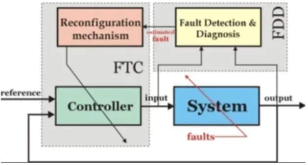
Quadrotor is a widely used UAV, since it is easy to develop. However, like any flying vehicle, a certification is mandatory to meet safety rules as far as failures and catastrophic effects are concerned. Therefore the fault tolerant control is of utmost importance in a quadrotor. The Fault-Tolerant Control System (FTCS) has the capacity to adapt itself to component faults automatically. In general, the FTCS can be classified into two types: Passive Fault-Tolerant Control Systems (PFTCS) and Active Fault-Tolerant Control Systems (AFTCS) [1]. In PFTCS, controllers are fixed and are designed to be robust against a class of foreseeable faults. These systems have limited fault-tolerant capabilities. In contrast to PFTCS, AFTCS react actively to system component failures by reconfiguring control actions so that the stability and acceptable performance of the whole system can be maintained. In this paper, we will focus on AFTCS, which include the Faults Detection and Diagnosis (FDD) and controller reconfiguration. A typical AFTCS structure is shown in Fig. 1.
The critical issue facing any AFTCS is that there is only a limited amount of reaction time available to perform fault detection, diagnosis and reconfiguration. The computational effort of different FTCS is of an important aspect [2].
The paper is organized as follows: in section II, an introduction of two model-based methods for fault detection and diagnosis is exposed. In section III, a case study of fault tolerant control for a quadrotor is developed.
*Resarch supported by Institut Supérieur de l'Aéronautique et de l'Espace (ISAE), 10 avenue Edouard Belin - BP 54032 31055 Toulouse cedex 4, France.
X. He was with ISAE (e-mail: [email protected]).
J.-C. Chaudemar, and F. Defaÿ are with ISAE (e-mail: [email protected], [email protected] ).
J. Huang is with the School of Aeronautic Science and Engineering, Beihang University, XueYuan Road No.37, HaiDian District, Beijing, China.
Figure 1. Fault-Tolerant Control System.
II. MODEL-BASED METHODS FOR FAULT DETECTION AND
DIAGNOSIS
Fault Detection and Diagnosis aims at recognizing a fault that has occurred and pinpointing one or more root causes of this fault. As it is well-known, an FDD scheme has three tasks: (1) fault detection indicates that something is wrong in the system; (2) fault isolation determines the location and the type of the fault; (3) fault identification determines the magnitude of the fault. Fault isolation and identification are usually referred as fault diagnosis in the literature [3], [7].
Generally speaking, the principal methods of FDD are based on the residual calculation, where the residuals signify the difference between the true value and the reference value of state variables. As the residual calculation always rely on the knowledge of models, so it is also called model-based method.
Model-based methods using residuals indicate potential faults in the system. From its mathematical model, one general assumption is that the residuals are changed significantly so that detection is possible with regard to the mostly inherent stochastic character. This means that the offset of the residuals after the occurrence of a fault is large enough and lasts long enough to be detectable. These model-based methods are classified as follows: parity equation, state estimation and parameter estimation techniques for generating residuals [4].
A. Parity equation
The basic idea of this approach is to take advantage of the coherence among the measurements. Thanks to analytical redundancy relations, a number of measurements are interrelated, thus residuals can be obtained by comparing the calculated value and the measured value [5]. These residuals enable fault detection and location.
Fault Tolerant Control of a Quadrotor based on Parameter Estimation
Techniques and use of a Reconfigurable PID Controller
*
Considering a linear continuous system, a mathematical model is described as follows:
𝑦(𝑡) = 𝐶𝑥(𝑡) + 𝑓(𝑡) (1)
where y(t) is the measurement, x(t) is the state and f(t) is the fault in the sensors.
If C is full-rank in column and the number of measurements is larger than the unknown state, then we can find a matrix V which is orthogonal to C. In this way, residual is given by (2).
𝑟(𝑡) = 𝑉𝑦(𝑡) = 𝑉𝐶𝑥(𝑡) + 𝑉𝑓(𝑡) = 𝑉𝑓(𝑡) (2)
This method is based on the static redundancy of system. However, the above conditions must be satisfied to apply this method, which makes it unsuitable for many practical cases. In order to extend its application, a method based on the dynamic redundancy is developed, without any restriction on the number of measurements.
Considering a linear continuous system, its mathematical model is given by:
{𝑥(𝑡)̇ = 𝐴𝑥(𝑡) + 𝐵𝑢(𝑡) + 𝑉𝑣(𝑡) + 𝐿𝑓(𝑡)
𝑦(𝑡) = 𝐶𝑥(𝑡) + 𝑁𝑛(𝑡) + 𝑀𝑓(𝑡) (3)
where n(t) are noise disturbances and v(t) unmeasurable inputs or disturbances. f(t) are additive faults.
If the variables in (3) are differentiable in q-order, then the matrix equation can be obtained in (4).
𝑌(𝑡) = 𝑇𝑥(𝑡) + 𝑄𝑢𝑈(𝑡) + 𝑄𝑣𝑉(𝑡) + 𝑄𝑛𝑁(𝑡) + 𝑄𝑓𝐹(𝑡) (4) with 𝑌(𝑡) = [ 𝑦(𝑡) 𝑦(𝑡)̇ ⋮ 𝑦(𝑞)(𝑡)] 𝑈(𝑡) = [ 𝑢(𝑡) 𝑢(𝑡)̇ ⋮ 𝑢(𝑞)(𝑡)] 𝑉(𝑡) = [ 𝑣(𝑡) 𝑣(𝑡)̇ ⋮ 𝑣(𝑞)(𝑡)] 𝐹(𝑡) = [ 𝑓(𝑡) 𝑓(𝑡)̇ ⋮ 𝑓(𝑞)(𝑡)] 𝑇 = [ 𝐶 𝐶𝐴 𝐶𝐴2 ⋮ 𝐶𝐴𝑞] 𝑄𝑢= [ 0 0 0 𝐶𝐵 0 0 𝐶𝐴𝐵 𝐶𝐵 0 ⋯ 00 0 ⋮ ⋱ ⋮ 𝐶𝐴𝑞−1𝐵 𝐶𝐴𝑞−2𝐵 𝐶𝐴𝑞−3𝐵 ⋯ 0] 𝑄𝑣= [ 𝑁 0 0 𝐶𝑉 𝑁 0 𝐶𝐴𝑉 𝐶𝑉 𝑁 ⋯ 00 0 ⋮ ⋱ ⋮ 𝐶𝐴𝑞−1𝑉 𝐶𝐴𝑞−2𝑉 𝐶𝐴𝑞−3𝑉 ⋯ 𝑁] 𝑄𝑓= [ 𝑀 0 0 𝐶𝐿 𝑀 0 𝐶𝐴𝐿 𝐶𝐿 𝑀 ⋯ 00 0 ⋮ ⋱ ⋮ 𝐶𝐴𝑞−1𝐿 𝐶𝐴𝑞−2𝐿 𝐶𝐴𝑞−3𝐿 ⋯ 𝑀]
By selecting matrix W such that
𝑊𝑇 = 0 𝑊𝑄𝑣= 0 (5)
a residual is obtained
𝑟(𝑡) = 𝑊𝑌(𝑡) − 𝑊𝑄𝑢𝑈(𝑡) = 𝑊𝑄𝑛𝑁(𝑡) + 𝑊𝑄𝑓𝐹(𝑡) (6)
So the residual is only influenced by the noise N(t) and the faults F(t). The noise influence can be eliminated by filtering and threshold fixing, so that the residual can detect only faults.
Considering a linear discrete system, its mathematical model is described in (7).
{𝑥(𝑘 + 1) = 𝐴𝑥(𝑘) + 𝐵𝑢(𝑘) + 𝑉𝑣(𝑘) + 𝐿𝑓(𝑘)
𝑦(𝑘) = 𝐶𝑥(𝑘) + 𝑁𝑛(𝑘) + 𝑀𝑓(𝑘) (7)
where n(k) are noise disturbances and v(k) unmeasurable inputs or disturbances. f(k) are additive faults.
If we can measure q samples consequently in the system described by (7), then the matrix equation can be obtained in (8). 𝑌(𝑘) = 𝑇𝑥(𝑘 − 𝑞) + 𝑄𝑢𝑈(𝑘) + 𝑄𝑣𝑉(𝑘) + 𝑄𝑛𝑁(𝑘) + 𝑄𝑓𝐹(𝑘) (8) with 𝑌(𝑘) = [ 𝑦(𝑘 − 𝑞) 𝑦(𝑘 − 𝑞 + 1) ⋮ 𝑦(𝑘) ] 𝑈(𝑘) = [ 𝑢(𝑘 − 𝑞) 𝑢(𝑘 − 𝑞 + 1) ⋮ 𝑢(𝑘) ] 𝑉(𝑘) = [ 𝑣(𝑘 − 𝑞) 𝑣(𝑘 − 𝑞 + 1) ⋮ 𝑣(𝑘) ] 𝑇 = [ 𝐶 𝐶𝐴 𝐶𝐴2 ⋮ 𝐶𝐴𝑞] 𝑄𝑢= [ 0 0 0 𝐶𝐵 0 0 𝐶𝐴𝐵 𝐶𝐵 0 ⋯ 00 0 ⋮ ⋱ ⋮ 𝐶𝐴𝑞−1𝐵 𝐶𝐴𝑞−2𝐵 𝐶𝐴𝑞−3𝐵 ⋯ 0] 𝑄𝑣= [ 𝑁 0 0 𝐶𝑉 𝑁 0 𝐶𝐴𝑉 𝐶𝑉 𝑁 ⋯ 00 0 ⋮ ⋱ ⋮ 𝐶𝐴𝑞−1𝑉 𝐶𝐴𝑞−2𝑉 𝐶𝐴𝑞−3𝑉 ⋯ 𝑁]
By selecting matrix W such that
𝑊𝑇 = 0 𝑊𝑄𝑣= 0 (9)
a residual is obtained
𝑟(𝑡) = 𝑊𝑌(𝑘) − 𝑊𝑄𝑢𝑈(𝑘) = 𝑊𝑄𝑛𝑁(𝑘) + 𝑊𝑄𝑓𝐹(𝑘) (10)
Sometimes the residuals become relatively large due to the noise and uncertainties in modeling. For instance, in non-linear systems, the residual are generated by using linearization methods [4].
B. Parameter estimation
The previous model-based method requires a precise model for fault detection. In many cases the models parameters are unknown or can only be known partly. Therefore, the parameter estimation method is required before applying another model-based method. The parameter estimation is considered as a model-based method to detect the faults as soon as the system parameters change due to faults.
By comparing linear and non-linear processes, the linear one is more frequently used because of its simplicity. Moreover, linearization techniques enable to tackle non-linear systems. For instance, let introduce the least square (LS) method.
Assuming the output at kTe , where Te is the sampling
time, we can estimate a measurement, as shown in (11).
𝑦̂𝑘= 𝜑𝑘𝑇𝜃 (11)
where 𝑦̂𝑘 is the estimation of output at kTe, 𝜑𝑘 is the
preceding measurements and 𝜃 is the parameter.
If there are a group of measurements and outputs, the (11) can be applied for every output, so the non-recursive least square parameter estimation can be realized in (12).
𝜃̂ = (∅𝑇∅)−1∅𝑇𝑌 (12)
with
∅ = [𝜑1 𝜑2 … 𝜑𝑘]𝑇
𝑌 = [𝑦1 𝑦2 … 𝑦𝑘]𝑇
From (12) we can easily know 𝜃̂ is influenced by the number of samples k, and the number of samples increases when the system works, so the recursive least square method can be deduced.
Assuming: 𝑃𝑁= (∅𝑇∅)−1= (∑𝑁𝑘=1𝜑𝑘𝜑𝑇𝑘)−1 (13)
𝑃𝑁+1−1 = 𝑃𝑁+1−1 + 𝜑𝑁+1𝜑𝑁+1𝑇 (14)
And the recursive least square parameter estimation is achieved in (15).
𝜃̂𝑁+1= 𝜃̂𝑁+ 𝑃𝑁+1𝜑𝑁+1𝑒𝑁+1 (15)
with
𝑒𝑁+1= 𝑦𝑁+1− 𝑦̂𝑁+1= 𝑦𝑁+1− 𝜑𝑁+1𝑇 𝜃̂𝑁 (16)
As calculating the inverse matrix is needed in the process of iteration, and it costs much computing resources to calculate the inverse matrix, so the matrix inversion lemma can be applied as shown in (17).
𝑃𝑁+1= 𝑃𝑁− 𝑃𝑁𝜑𝑁+1(𝜑𝑁+1𝑇 𝑃𝑁𝜑𝑁+1+ 1)−1𝜑𝑁+1𝑇 𝑃𝑁 (17)
So the improved recursive method is shown as (18).
{ 𝑃𝑁+1= 𝑃𝑁−
𝑃𝑁𝜑𝑁+1𝜑𝑁+1𝑇 𝑃𝑁
1+𝜑𝑁+1𝑇 𝑃𝑁𝜑𝑁+1
𝜃̂𝑁+1= 𝜃̂𝑁+ 𝑃𝑁+1𝜑𝑁+1(𝑦𝑁+1− 𝜑𝑁+1𝑇 𝜃̂𝑁)
(18)
To start the recursive estimator we need to initialize θ̂N
and PN. If there is no information about it, we can set θ̂N= 0,
PN= αI where α ≫ 1.
This estimator is optimal to minimize the equation 𝐽 = ∑𝑁+1𝑘=1(𝑦𝑘− 𝑦̂𝑘)2, which assumes all the measurements
are of the same importance. For time-varying process, it is not true. So a forgetting factor should be added to put more emphasis on the recent measurements, as shown in the (19). The forgetting factor 𝜆 signifies the importance of recent measurement compared to further measurements. Such estimator is optimal to minimize the equation:
𝐽 = ∑𝑁+1𝑘=1(𝑦𝑘− 𝑦̂𝑘)2𝜆𝑁+1−𝑘 { 𝑃𝑁+1= 𝜆−1(𝑃𝑁− 𝑃𝑁𝜑𝑁+1𝜑𝑁+1𝑇 𝑃𝑁 𝜆+𝜑𝑁+1𝑇 𝑃𝑁𝜑𝑁+1) 𝜃̂𝑁+1= 𝜃̂𝑁+ 𝑃𝑁+1𝜑𝑁+1(𝑦𝑁+1− 𝜑𝑁+1𝑇 𝜃̂𝑁) (19)
In practice, the parameter estimation only needs the model structure and is suitable for both additive and multiplicative faults, but its computational effort is tough [4]. It is important to point out that the two methods are not isolated, and they can be combined to realize a better performance.
III. CASE STUDY OF A QUADROTOR
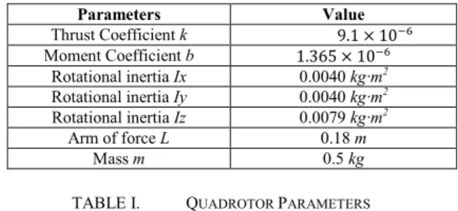
Parameters Value Thrust Coefficient k 9.1 × 10⁻⁶ Moment Coefficient b 1.365 × 10⁻⁶ Rotational inertia Ix 0.0040 kg·m2 Rotational inertia Iy 0.0040 kg·m2 Rotational inertia Iz 0.0079 kg·m2 Arm of force L 0.18 m Mass m 0.5 kg
TABLE I. QUADROTOR PARAMETERS
The parameters of the quadrotor used in this paper are shown in table I. In this paper, dynamics model and measurement model will be given at first. Then PID controller will be introduced briefly. At last, faults in a rotor will be considered, which will influence the thrust coefficient k (unit 𝑁/ (𝑟𝑎𝑑/𝑠)2) and moment coefficient b (unit 𝑁 · 𝑚/(𝑟𝑎𝑑/𝑠)2).
FDD and controller reconfiguration mechanism will be designed for the fault.
A. Dynamics and Measurement
Before giving the dynamics model, let define the coordinate system. As shown in Fig. 2, body coordinate system and inertial coordinate system are introduced, and vectors in one system can be transformed to ones in another system by multiplying them with transformation matrix. The rotation sequence from the inertial system to the body system is z, y and x. The forces concerned are the gravity of quadrotor and the lifts of the four rotors, and the moments concerned are the torques of the four rotors, while other forces and moments are too small to be considered [6], [9].
TABLE II. MEASUREMENT PARAMETERS
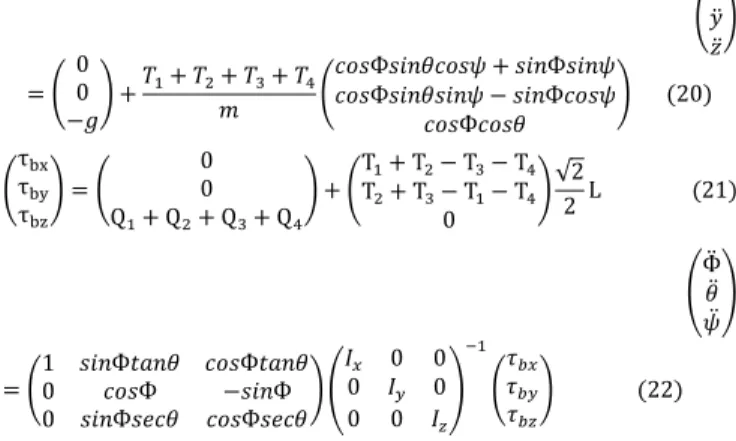
Dynamics model are given from (20) to (22). 𝜏𝑏𝑥, 𝜏𝑏𝑦, 𝜏𝑏𝑧
are the moments of the quadrotor in the body coordinate system, and Ф, 𝜃, 𝜓 are roll angle, pitch angle and yaw angle respectively. (𝑥̈𝑦̈ 𝑧̈ ) = ( 0 0 −𝑔) + 𝑇1+ 𝑇2+ 𝑇3+ 𝑇4 𝑚 ( 𝑐𝑜𝑠Ф𝑠𝑖𝑛𝜃𝑐𝑜𝑠𝜓 + 𝑠𝑖𝑛Ф𝑠𝑖𝑛𝜓 𝑐𝑜𝑠Ф𝑠𝑖𝑛𝜃𝑠𝑖𝑛𝜓 − 𝑠𝑖𝑛Ф𝑐𝑜𝑠𝜓 𝑐𝑜𝑠Ф𝑐𝑜𝑠𝜃 ) (20) ( τbx τby τbz ) = ( 0 0 Q1+ Q2+ Q3+ Q4 ) + (TT12+ T+ T23− T− T31− T− T44 0 )√2 2 L (21) (Ф̈𝜃̈ 𝜓̈ ) = (1 𝑠𝑖𝑛Ф𝑡𝑎𝑛𝜃 𝑐𝑜𝑠Ф𝑡𝑎𝑛𝜃0 𝑐𝑜𝑠Ф −𝑠𝑖𝑛Ф 0 𝑠𝑖𝑛Ф𝑠𝑒𝑐𝜃 𝑐𝑜𝑠Ф𝑠𝑒𝑐𝜃) ( 𝐼𝑥 0 0 0 𝐼𝑦 0 0 0 𝐼𝑧 ) −1 ( 𝜏𝑏𝑥 𝜏𝑏𝑦 𝜏𝑏𝑧 ) (22)
In addition, the motor response model should be included, as shown in equation (23).
𝜔(𝑠) = 𝜔𝑐𝑜𝑛(𝑠)
1
0.05𝑠 + 1 (23)
Measurement model is also constructed to take the noise into account. The sensors consist of accelerometers, gyroscopes and GPS. Accelerometer and gyroscope parameters are shown in Table II, while the bias of the gyroscope is so small that it is neglected. To simplify the problem, GPS is considered to be accurate and is used for the calibration of positon and velocity every 0.25s (4Hz).
As measurements of accelerometer and gyroscope are in the body coordinate system, the navigation system needs to get the position and attitude in the earth coordinate system. We could use equation (24) and (25) to estimate the angular velocity and acceleration. Attitude, velocity and positon can be obtained by integration. As the bias of measurement exists in accelerometer, the calibration of velocity and position will be applied with the help of GPS.
( Ф̇𝑒 𝜃̇𝑒 𝜓̇𝑒 ) = ( 1 𝑠𝑖𝑛Ф𝑒𝑡𝑎𝑛𝜃𝑒 𝑐𝑜𝑠Ф𝑒𝑡𝑎𝑛𝜃𝑒 0 𝑐𝑜𝑠Ф𝑒 −𝑠𝑖𝑛Ф𝑒 0 𝑠𝑖𝑛Ф𝑒𝑠𝑒𝑐𝜃𝑒 𝑐𝑜𝑠Ф𝑒𝑠𝑒𝑐𝜃𝑒) ( 𝑝𝑚 𝑞𝑚 𝑟𝑚 ) = ( 1 𝑠𝑖𝑛Ф𝑒𝑡𝑎𝑛𝜃𝑒 𝑐𝑜𝑠Ф𝑒𝑡𝑎𝑛𝜃𝑒 0 𝑐𝑜𝑠Ф𝑒 −𝑠𝑖𝑛Ф𝑒 0 𝑠𝑖𝑛Ф𝑒𝑠𝑒𝑐𝜃𝑒 𝑐𝑜𝑠Ф𝑒𝑠𝑒𝑐𝜃𝑒 ) 𝜔 (24) ( ẍ𝑒 ÿ𝑒 z̈𝑒 ) = ( 0 0 −g) +
(cos𝜃𝑒cosψ𝑒sinψcos𝜃𝑒 sinФ𝑒sin𝜃𝑒cosψ𝑒sinψsin𝜃𝑒sinФ𝑒+ cosФ𝑒cosψ𝑒− sinψ𝑒cosФ𝑒 cosФ𝑒sin𝜃𝑒cosψ𝑒cosФ𝑒sin𝜃𝑒sinψ𝑒− sinФ𝑒cosψ𝑒+ sinФ𝑒sinψ𝑒
−sin𝜃𝑒 cos𝜃𝑒sinФ𝑒 cosФ𝑒cos𝜃𝑒 ) (
ẍm ÿm z̈m) (25)
To estimate the quadrotor’s moment, angular acceleration is estimated by equation (26). Here ωn signifies the
measurement of gyroscope in time nT, T being the sampling time of the gyroscope.
𝜔̇𝑛−1=
1
2𝑇(𝜔𝑛− 𝜔𝑛−2) (26)
B. PID Controller
PID controller for position control is designed for the quadrotor and it is achieved through two steps. The first step is the attitude control, and the second step is the position control, as shown in Fig.3 and Fig. 4. We need to restructure the dynamics model through equation (27). Combined with equation (20), U1, desired roll angle Ф∗ and desired pitch
angle 𝜃∗ can be expressed by desired yaw angle 𝜓∗ and
desired acceleration in three axes, which corresponds to the block parameter calculation in Fig. 3.
{ 𝑈1= 𝑇1+ 𝑇2+ 𝑇3+ 𝑇4 𝑈2= (𝑇1+ 𝑇2− 𝑇3− 𝑇4) √2 2 𝐿 𝑈3= (𝑇2+ 𝑇3− 𝑇1− 𝑇4)√22 𝐿 𝑈4= 𝑄1−𝑄2+ 𝑄3− 𝑄4 (27)
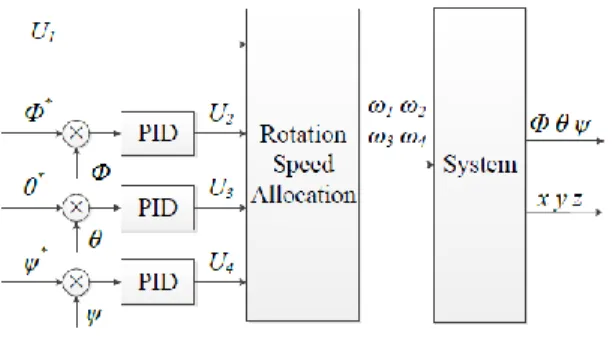
The thrusts and moments of rotors can be obtained in equation (28). Combined with equation (27), the desired rotation speed of motor can be determined, which corresponds to the block rotation speed allocation in Fig. 4.
{𝑇𝑖= 𝑘𝜔𝑖2
𝑄𝑖= 𝑏𝜔𝑖2
𝑖 = 1,2,3,4 (28)
Figure 3. Position Control
Accelerometer Noise 2.0 × 10⁻⁴𝑚2/𝑠4 Bias 5.0 × 10⁻⁴𝑚/𝑠3 Sampling Frequency 105.5Hz Gyroscope Noise 2.0 × 10⁻⁷𝑚2/𝑠4 Bias Neglected Sampling Frequency 105.5Hz
Figure 4. Attitude Control
Parameters of the PID controller are fixed then tests are made. This controller show short response time, satisfying precision and enough robustness. However, when faults in rotor happen, the flight fluctuates a lot although it becomes stable at last. Such result can be optimized by FTCS, which will be shown after. The simulation result will be compared to prove the advantage of FTCS.
C. Fault Detection and Diagnosis
In this paper, only the rotor fault is considered. This fault corresponds to the deformation, damage, wreckage of blade, which changes the thrust coefficient k and moment coefficient b. As the model structure is already known and this fault changes model parameters, we choose parameter estimation techniques to detect and diagnose the fault. [8] To simplify the problem, two hypotheses are made: (1) the fault is static, which means the parameter only changes from one constant to another constant after the fault appears; (2) it is impossible to appear two faults simultaneously.
We will use equation (29) to detect and diagnose the fault. From the equation, we can see that we need the real motor rotation speed, the total thrust and the moment in three axes. Real motor rotation speed 𝜔 can be calculated from control signal 𝜔𝑐𝑜𝑛 if there is no fault in motor, as shown in
equation (4). The total thrust can be obtained from the estimated acceleration in the earth coordinate system, and the moment in three axes can be obtained from the estimated angular acceleration in the body coordinate system.
{ 𝑇 = 𝑘1𝜔12+ 𝑘2𝜔22+ 𝑘3𝜔32+ 𝑘4𝜔42 𝜏𝑏𝑥= (𝑘1𝜔12+ 𝑘2𝜔22− 𝑘3𝜔32− 𝑘4𝜔42) √2 2 𝐿 𝜏𝑏𝑦= (𝑘2𝜔22+ 𝑘3𝜔23− 𝑘1𝜔12− 𝑘4𝜔42) √2 2𝐿 𝜏𝑏𝑧= 𝑏1𝜔12− 𝑏 2𝜔22+ 𝑏3𝜔32− 𝑏4𝜔42 (29)
There are eight unknown variables and only four equations, so it is necessary to use recursive least square estimators to estimate the unknowns. [5] Traditionally, the thrust coefficients can be estimated by the first three equations and the moment coefficients can be estimated by the last one. The four thrust coefficients (or moment coefficients) are estimated all at once, which make its
estimation inaccurate with the existence of noise. To eliminate the influence of noise, a new parameter estimation method is proposed which combines the recursive least square estimators and a logical reasoning. In this paper and for the quadrotor case, the variation of rotational speed is very small compared to the set point (less than 10%), so the influence of the square term can be neglected for a first approximation.
The first step is to detect the fault. The detection is achieved through the estimation of thrust coefficient. For a certain rotor, for example, rotor 1, the first three equations of (29) can be written as equation (30).
{ 𝑘1𝑎= 𝑇 − 𝑘2𝜔22− 𝑘3𝜔32− 𝑘4𝜔42 𝜔12 𝑘1𝑏= √2𝜏𝑏𝑥 𝐿 − 𝑘2𝜔22+ 𝑘3𝜔32+ 𝑘4𝜔42 𝜔12 𝑘1𝑐= −√2𝜏𝐿𝑏𝑦+ 𝑘2𝜔22+ 𝑘3𝜔32− 𝑘4𝜔42 𝜔12 (30)
If there is no fault or the fault is only in rotor 1, the thrust coefficient of other rotors is determined and already known, and the thrust coefficient of rotor 1 calculated by the three equations will always be the same (or fluctuate in reasonable interval under noise). Otherwise, the three results will be very different. (Note: such conclusion is made based on the assumption of single fault) To reduce the fluctuation of estimation results, we introduce a recursive least square estimator with forgetting factor 0.9 for each equation. Until now, the detection logic is clear: if the thrust coefficients calculated by the three equations respectively are close, the estimation is reliable and we can check the estimation to diagnosis the fault; otherwise, the fault must be in other rotor. If we apply such process to each rotor, we can locate the fault and estimate the thrust coefficient. After we locate the fault, we can estimate the moment coefficient of the rotor with fault by the last equation in (29). This process is also achieved by the recursive least square estimator.
Simulation is made to test the performance. We suppose that the fault happens in rotor 1 at t=5s, which makes 𝑘1 get
4.55 × 10⁻⁶ from 9.1 × 10⁻⁶, and 𝑏
1 get 0.6825 × 10⁻⁶
from 1.365 × 10⁻⁶. Simulation results are shown in Fig. 5
and 6. The fault is precisely detected and diagnosed in less than 0.2 seconds.
Figure 5. FDD Results for Thrust Coefficient
Figure 6. FDD Results for Moment Coefficient
D. Controller Reconfiguration
The controller will be reconfigured after the fault occurs. As forementioned, motors’ rotation speeds are allocated based on equation (27) and equation (28). After the fault occurrence, thrust coefficient k and moment coefficient b in equation (28) should be adjusted to the diagnosis results and the allocated rotation speed should be recalculated to adapt to the new situation. So the new approach of rotation speed allocation is shown in the following equation.
[ 𝜔12 𝜔22 𝜔32 𝜔42] = [ 𝑘1 𝑘2 √2 2 𝑘1𝐿 √22𝑘2𝐿 𝑘3 𝑘4 −√2 2 𝑘3𝐿 −√22 𝑘4𝐿 −√2 2 𝑘1𝐿 √22 𝑘2𝐿 𝑏1 −𝑏2 √2 2𝑘3𝐿 −√22𝑘4𝐿 𝑏3 −𝑏4 ] −1 [ 𝑈1 𝑈2 𝑈3 𝑈4 ] (31)
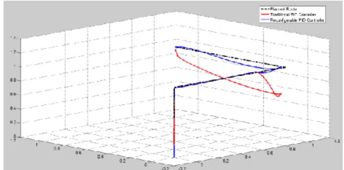
Simulation is made to test the performance. We suppose that the waypoints for the quadrotor maneuver are (0,0,0), (0,0,1), (1,0,1), (1,1,1), and the fault occurs in rotor 1 at t=5s, which makes 𝑘1 get 4.55 × 10⁻⁶ from 9.1 × 10⁻⁶, and
𝑏1 get 0.6825 × 10⁻⁶ from 1.365 × 10⁻⁶. A comparison is
made between a traditional PID controller and this fault tolerant controller. We can see the fault tolerant controller
works better than traditional one. Currently, this adaptive PID is designed manually.
Figure 7. Fault Tolerant Control Results
IV. CONCLUSION
This paper has proposed a fault-tolerant control method which includes a fault detection and diagnosis approach for the rotor fault of quadrotor and develops a reconfigurable PID controller. This method successfully improves the performance of quadrotor under fault, as shown in our simulation. Future work will be done to develop new fault-tolerant control method which can cope with more faults and enables an automatic adjustment of the controller in real time.
REFERENCES
[1] Mahmoud, Magdi S., and Yuanqing Xia. “Analysis and Synthesis of Fault-tolerant Control Systems”. John Wiley & Sons, 2013.
[2] Jiang, Jin.“Fault-tolerant control systems - an introductory overview”. Acta Automatica Sinica, 2005, vol. 1. [3] Zhang, Youmin, and Jin Jiang. "Bibliographical review on
reconfigurable fault-tolerant control systems." Annual reviews in control 32.2 (2008): 229-252.
[4] Isermann, Rolf. “Fault-diagnosis systems: an introduction from fault detection to fault tolerance”. Springer Science & Business Media, 2006.
[5] Toscano, Rosario. "Commande et diagnostic des systèmes dynamiques." Elipses, Paris (2005).
[6] Beard, Randal W. "Quadrotor dynamics and control." Brigham Young University (2008).
[7] Zhang, Youmin, and Jin Jiang. "Bibliographical review on reconfigurable fault-tolerant control systems." Annual reviews in control 32.2 (2008): 229-252.
[8] Isermann, Rolf. Fault-diagnosis systems: an introduction from fault detection to fault tolerance. Springer Science & Business Media, 2006.
[9] Y. M. Zhang, A. Chamseddine, C. A. Rabbath, B. W. Gordon, C.-Y. Su, S. Rakheja, C. Fulford, J. Apkarian, and P. Gosselin. “Development of Advanced FDD and FTC Techniques with Application to an Unmanned Quadrotor Helicopter Testbed”. Journal of the Franklin Institute, vol. 350, no. 9, pp. 2396-2422, 2013.