an author's
https://oatao.univ-toulouse.fr/26592
https://doi.org/10.1016/j.spl.2020.108893
Besson, Olivier and Vincent, François and Gendre, Xavier A Stein’s approach to covariance matrix estimation using
regularization of Cholesky factor and log-Cholesky metric. (2020) Statistics & Probability Letters, 167. 1-9. ISSN
0167-7152
A Stein’s approach to covariance matrix estimation using
regularization of Cholesky factor and log-Cholesky metric
Olivier Besson
∗, François Vincent, Xavier Gendre
ISAE-SUPAERO, University of Toulouse, 10 Avenue Edouard Belin, 31055 Toulouse, FranceKeywords:
Cholesky factor
Covariance matrix estimation Regularization
Steins’s estimation
a b s t r a c t
We consider a Stein’s approach to estimate a covariance matrix using regularization of the sample covariance matrix Cholesky factor. We propose a method to estimate accurately the regularization vector which minimizes the risk associated with the recently introduced log-Cholesky metric.
1. Introduction and problem statement
Covariance matrix (CM) estimation is at the core of most methods used to process multichannel data, in a wide variety of applications, including social science, life science, physics, engineering, finance. The estimation of the covariance matrix is indeed needed for the most widely used tools of multivariate analysis, e.g., principal component analysis, adaptive detection, filtering (Scharf,1991; Pourahmadi,2013;Srivastava,2002). Under the Gaussian assumption, the maximum likelihood estimate (MLE) of the covariance matrix is the sample covariance matrix (SCM) S
=
XXTwhere X is the p×
ndata matrix where columns of X are assumed to be independent and to follow a normal distribution with zero mean and covariance matrixΣ. Unfortunately, when the number of observations n is not significantly larger than the observation size p, S has been observed to be much less well-conditioned thanΣ. More precisely, large eigenvalues ofΣtend to be over-estimated while small eigenvalues tend to be under-estimated. Therefore, there has been a natural need to somehow regularize the SCM.
The literature about this problem is huge. However, the approach proposed byStein(1956,1986),James and Stein
(1992) has markedly emerged and influenced a great deal of research, see e.g.,Haff(1979,1980), Dey and Srinivasan
(1985,1986),Perron(1992),Ledoit and Wolf(2004),Ma et al.(2012) andTsukuma(2016) and references therein. The basic principle of Stein’s approach is to define a loss function and to minimize its average value, referred to as the risk, within a given class of estimatesΣ
ˆ
. Three main classes of estimates have been considered: regularization of theeigenvalues of the SCM, regularization of its Cholesky factor or shrinkage. The first class involves estimates of the form
ˆ
Σ
=
Udiag(ϕ
(λ
))UTwhere S=
Udiag(λ
)UTdenotes the eigenvalue decomposition of the SCM andϕ
(λ
) is some non-linearfunction of the eigenvalues
λ
. For the riskL1(Σ, ˆ
Σ)=
Tr{ ˆ
ΣΣ−1} −
log det(ΣΣˆ
−1)−
p, it was proposed to minimize anunbiased estimate of the corresponding risk, this unbiased estimate being obtained from the so-called Stein–Haff identity for Wishart matrices (Haff,1979), or using the distribution of
λ
(Sheena,1995). It turns out that this procedure results∗ Corresponding author.
E-mail addresses: [email protected](O. Besson),[email protected](F. Vincent),[email protected]
(X. Gendre).
2
in some eigenvalues ofΣ
ˆ
being negative and, moreover, it does not preserve the order of the eigenvalues inλ
. This means that it can be improved upon by an estimator which preserves the order (Sheena and Takemura,1992). In order to overcome these problems, Stein proposed an isotonizing scheme which guarantees that the eigenvaluesϕ
(λ
) are all positive and in decreasing order, seeLin and Perlman(1985) for details. Note that Ledoit and Wolf, applying to the theory of large-dimensional asymptotics, proposed a procedure that alleviates all above mentioned problems and minimizes an unbiased estimate of the risk, in the spirit of Stein’s approach (Ledoit and Wolf,2018).Another class of estimates amounts to shrinkage of the SCM to the identity matrix, leading to estimates of the form
ˆ
Σ
=
a[
S+
bI]
where a and b are regularizing parameters. One of the fundamental works is due toHaff (1980) who considered b=
g(Tr{
S−1}
) and an empirical Bayes approach but this approach triggered the highest number of studies,see e.g.,Ledoit and Wolf(2004),Konno(2009),Chen et al.(2010),Coluccia(2015) andIkeda et al.(2016) and references therein.
However, the first class of estimates considered by Stein was that based on the regularization of the Cholesky factor of S, i.e., estimates of the formΣ
ˆ
=
GSdiag(d)GTS where GS is the Cholesky factor of S. Stein showed that, for the lossL1(Σ
, ˆ
Σ), the corresponding riskR1(Σ,
d)=
E{
L1(Σ, ˆ
Σ)}
is minimized when[
d1]
j=
(p−
j+
E{
χ
n2−j+1}
)−1 (1)
The optimal vector, say d2, which minimizesR2(Σ
,
d)=
E{
L2(Σ, ˆ
Σ)}
whereL2(Σ, ˆ
Σ)=
Tr{
(ΣΣˆ
−1−
In)2}
was derivedby Selliah inSelliah(1964). InTsukuma and Kubokawa(2016) extensions of these estimators to the case p
<
n are given. Using estimates of the typeΣˆ
=
GSdiag(d)GTSis interesting for some reasons. First, the Cholesky factor is easy to compute.Furthermore, it is of interest when used for whitening purposes: indeed, in order to whiten data, only a triangular system of equations needs to be solved. Whitening is particularly useful when detecting a signal of interest among noise with covariance matrixΣsince the optimal detection scheme involves whitening followed by matched filtering (Scharf,1991). Now, since estimation of the Cholesky factor may be interested per se, it is natural to consider risk functions that are expressed in terms of the Cholesky factor. This is what was proposed byEaton and Olkin(1987) who considered the two following loss functions
L3(GΣ
,
GΣˆ)=
Tr{
(G −1 ΣGΣˆ−
I)(G −1 ΣGΣˆ−
I)T}
(2) L4(GΣ,
GΣˆ)=
Tr{
(G −1 ˆ ΣGΣ−
I)(G −1 ˆ ΣGΣ−
I) T}
(3)and associated risksR3(GΣ
,
d)=
E{
L3(GΣ,
GΣˆ)}
andR4(GΣ,
d)=
E{
L4(GΣ,
GΣˆ)}
. They showed that the optimal d, whichminimize these risks, are respectively
[
d3]
1j/2=
E{
√
χ
2 n−j+1}
p−
j+
E{
χ
2 n−j+1}
(4)[
d4]
1/2 j=
n−
1 (n−
j)(n−
j−
1) 1 E{
(χ
n2−j+1) −1/2}
(5)In this letter, we investigate estimates of the formΣ
ˆ
=
GSdiag(d)GTS and we focus on a loss function that depends onthe Cholesky factor. More precisely, we consider a recently proposed distance in the set of lower triangular matrices with positive diagonal entries. We show that the optimal regularization vector depends onΣand we propose a procedure to find an accurate approximation. Finally, we evaluate the four approaches mentioned above as well as our new method on a relevant metric which is related to the natural distance between covariance matrices.
Notations. The jth entry of a vector d is denoted djor
[
d]
jand we sometimes use d=
vect(dj). The (i,
j)-th entry of ap
×
p matrix M is either denoted by Mijor[
M]
ij. We let diag(M) be the p×
1 vector whose entries are Mjj. Conversely,for any vector d, diag(d) is a diagonal matrix whose diagonal entries are dj. We will sometimes note diag(dj). ddiag(M)
is defined as ddiag(M)
=
diag(diag(M)).⊙
is the Hadamard product, i.e., element-wise product. The Cholesky factor of matrixΣwill be denoted GΣ, i.e., GΣ is lower-triangular with positive diagonal entries and GΣGTΣ=
Σ.N(
µ, σ
2)
denotes the normal distribution with mean
µ
and varianceσ
2.χ
2qstands for the chi-square distribution with q degrees of
freedom andWp
(
n,
Σ)
stands for the Wishart distribution with n degrees of freedom and parameter matrixΣ.=
d means ‘‘is distributed as’’.In the paper, we will need the following result on some statistics associated with GW¯ whereW
¯
d
=
Wp(
n,
I)
. This result stems from the fact that all entries of GW¯ are independent with[
GW¯]
ijd
=
N(
0,
1)
for i>
j and[
GW¯]
jj d=
√
χ
2 n−j+1(Muirhead, 1982;Gupta and Nagar,2000).Result 1. For any matrix M, E
{
MGW¯} =
Mdiag(E{
√
χ
2n−j+1
}
) which implies that E{
[
MGW¯]
jj} = [
M]
jjE{
√
χ
2 n−j+1}
. AdditionallyE
{
GTW¯MGW¯}
is a diagonal matrix given by[
E{
GTW¯MGW¯}
]
jj=
E{
χ
2 n−j+1}
Mjj+
p∑
i=j+1 Mii (6)2. Minimization of risk function associated with log-Cholesky metric
As stated above, we consider here a new Riemannian metric, termed log-Cholesky metric, defined on the set of lower triangular matrices with positive diagonal entries as (Lin,2019):
L5(GΣ
,
GΣˆ)=
∑
i>j([
GΣˆ]
ij− [
GΣ]
ij)
2+
p∑
j=1(
log[
GΣˆ]
jj−
log[
GΣ]
jj)
2=
GΣˆ−
GΣ
2 F−
diag(GΣˆ)−
diag(GΣ)
2+
log diag(GΣˆ)−
log diag(GΣ)
2(7) Since GΣˆ
=
GΣGW¯D1/2, one has
GΣˆ−
GΣ
2 F=
Tr{
(GΣˆ−
GΣ)(GΣˆ−
GΣ)T}
=
Tr{
GΣ(GW¯D1/2−
I)(GW¯D1/2−
I)TGTΣ}
=
Tr{
GΣGW¯DGTW¯G T Σ} −
2Tr{
GΣGW¯D1/2GTΣ} +
Tr{
Σ}
=
√
dTddiag(GTW¯G T ΣGΣGW¯)√
d−
2√
dTdiag(GTΣGΣGW¯)+
Tr{
Σ}
(8) Moreover, since[
GΣˆ]
jj=
d 1/2 j[
GΣGW¯]
jj, one has
diag(GΣˆ)−
diag(GΣ)
2=
p∑
j=1 (d1j/2[
GΣGW¯]
jj− [
GΣ]
jj)2=
√
dTddiag(GΣGW¯⊙
GΣGW¯)√
d−
2√
dTdiag(GΣGW¯⊙
GΣ)+ ∥
diag(GΣ)∥
2 (9) and
log diag(GΣˆ)−
log diag(GΣ)
2=
p∑
j=1 (log d1j/2+
log[
GW¯]
jj)2=
(log√
d)T(log
√
d)+
2(log√
d)Tlog diag(G¯ W)
+
log diag(GW¯)
2 (10) Gathering the previous equations yields the following expression forL5(Σ, ˆ
Σ):L5(GΣ
,
GΣˆ)=
√
dT[
ddiag(GTW¯G T ΣGΣGW¯)−
ddiag(GΣGW¯⊙
GΣGW¯)]
√
d−
2√
dT[
diag(GTΣGΣGW¯)−
diag(GΣGW¯⊙
GΣ)]
+
(log√
d)T(log√
d)+
2(log√
d)Tlog diag(GW¯)+
Tr{
Σ} − ∥
diag(GΣ)∥
2+
log diag(GW¯)
2 (11) It ensues that the corresponding risk is given byR5(GΣ
,
d)=
E{
L5(GΣ,
GΣˆ)}
=
√
dTdiag(a)√
d−
2√
dTb+
(log√
d)T(log√
d)+
2(log√
d)Tc+
Tr{
Σ} − ∥
diag(GΣ)∥
2+
E{
log diag(GW¯)
2}
(12) with a=
E{
diag(GTW¯GTΣGΣGW¯)} −
E{
diag(GΣGW¯⊙
GΣGW¯)}
b=
E{
diag(GTΣGΣGW¯)} −
E{
diag(GΣGW¯⊙
GΣ)}
c=
E{
log diag(GW¯)}
(13)The jth elements of these vectors are given by aj
=
E{
χ
n2−j+1}
([
GTΣGΣ]
jj− [
GΣ]
2jj) +
p∑
i=j+1[
GT ΣGΣ]
ii bj=
E{
√
χ
2 n−j+1}
([
GTΣGΣ]
jj− [
GΣ]
2jj)
cj=
E{
log√
χ
2 n−j+1}
(14)4
Table 1
Average value of RRI5(Σ,d)= [R5(GΣ,d)−R5(GΣ,d5(Σ))]/R5(GΣ,d5(Σ)).
p, n d=d5(Ip) d= ˆd5
p=16, n=p+2 13.32% 0.56%
p=16, n=2p 11.08% 0.09%
p=64, n=p+2 17.38% 0.18%
p=64, n=2p 12.45% 0.03%
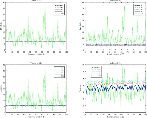
Fig. 1. Risks of the various estimators over 100 random trials ofΣ. p=16 and n=p+2.
It can be observed thatR5(GΣ
,
d) depends on GΣ. Note also that, in order to minimize this risk, we need to minimizeover R+
functions of the form
fj(x)
=
ajx2−
2bjx+
log2x+
2cjlog x We have f′ j(x)=
2ajx−
2bj+
2x−1log x+
2cjx−1=
2x−1[
ajx2−
bjx+
log x+
cj]
=
2x−1gj(x) (15) Differentiating gj(x) yields gj′(x)=
x−1(2ajx2−
bjx+
1)It can be readily shown that gj′(x)
>
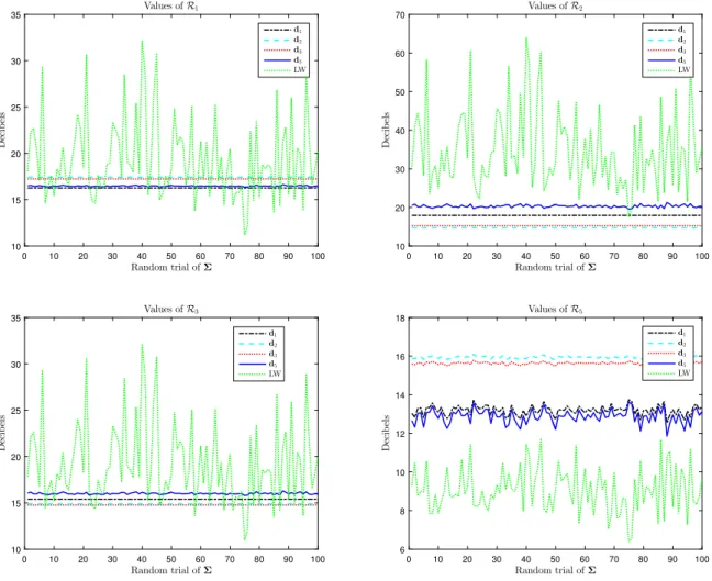
0 given the values of ajand bj, which implies that gj(x) is monotonically increasingFig. 2. Risks of the various estimators over 100 random trials ofΣ. p=16 and n=2p.
f′
j(x⋆j)
=
0. Since gj(x)<
0 for x<
x⋆j, it follows that fj(x) achieves its unique minimum at x⋆j. Therefore, the risk isminimized for d1j/2
=
x⋆j. We let d5(Σ) be the optimal vector for this log-Cholesky distance, where we emphasize that thisvector depends onΣ.
Since the optimal regularizing matrix depends on Σwhich is unknown, the usual procedure is to resort to Stein unbiased risk estimation (SURE), that is to find a functionL
ˆ
5(d,
S) such that E{ ˆ
L5(d,
S)} =
R5(GΣ,
d), or at least such thatE
{ ˆ
L5(d,
S)}
coincides with the part ofR5(GΣ,
d) that depends on d, and to minimizeLˆ
5(d,
S). In our case, this amountsto obtain unbiased estimates of a and b. Since one has E
{[
GTSGS]
jj} =
E{
χ
n2−j+1}[
G T ΣGΣ]
jj+
p∑
i=j+1[
GTΣGΣ]
ii E{[
GS]
2jj} =
E{
χ
n2−j+1}[
GΣ]
2jjit is clear that a
ˆ
j= [
GTSGS]
jj− [
GS]
2jj is an unbiased estimate of aj. However, finding an unbiased estimate of bjturnsout to be more problematic because an unbiased estimate of
[
GTΣGΣ]
jjdoes not seem feasible to obtain because of theterm
∑
pi=j+1
[
GTΣGΣ]
iiin E{[
GTSGS]
jj}
. Moreover, minimizing an estimateLˆ
5(d,
S) instead ofR5(GΣ,
d) unavoidably leadsto performance loss. Therefore, we investigate alternative solutions here.
A first straightforward method comes from the observation that, for all other lossesRi(Σ
,
d), i=
1, . . . ,
4, the optimal vector di(Σ) does not depend onΣand can be computed as di(Ip). Therefore, one can choose d5(Ip) as the regularizationvector. This solution is very simple, yet one needs to study how far is the risk associated with d5(Ip) from the risk obtained
with the optimal solution d5(Σ). In case the risk increase is not very important, using d5(Ip) is much simpler than an
approximate SURE approach and may perform as well.
However, one can anticipate some loss of performance of d5(Ip) compared to d5(Σ). To remedy this problem, we use
the fact thatR5(GΣ
,
d) and its minimizer depend onΣand we suggest an alternative approach which consists in findingd as the minimizer ofR5(GΣˆ
,
d) whereΣˆ
is some estimate ofΣ. For instance, one could useΣˆ
=
n−1S. Then, one obtainsˆ
6
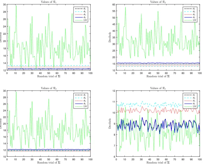
Fig. 3. Risks of the various estimators over 100 random trials ofΣ. p=64 and n=p+2.
ˆ
d(0)5 be some initial vector, for instanced
ˆ
(0)5=
d5(Ip) ordˆ
(0)5=
n−1/21
p where 1pis a length-p vector whose elements
are all equal to one, andΣ
ˆ
(0)=
GSdiag(d
ˆ
(0)5 )GTS. Then, for n=
1, . . .
, one can compute dˆ
(n)
5
=
arg mindR5(GΣˆ(n−1),
d)andΣ
ˆ
(n)=
GSdiag(d
ˆ
(n)5 )GTS. We letdˆ
5 be the vector at the end of the iterations. It is our experience that these iterationsconverge rather fast and that, typically, 5 iterations are sufficient.
In order to evaluate the difference betweenR5(GΣ
,
d5(Σ)),R5(GΣ,
d5(I)) andR5(GΣ, ˆ
d5) we conducted the followingexperiment. A large number of matricesΣwere drawn at random asΣ
=
Udiag(λ
)UT where U is uniformly distributedover the set of unitary matrices, and
λ
jare independent random variables drawn uniformly on ]0,
1]. For each matrixΣ,the optimal d5(Σ) was computed along with the corresponding risk. The relative risk increase RRI5(Σ
,
d)= [
R5(GΣ,
d)−
R5(GΣ,
d5(Σ))]
/
R5(GΣ,
d5(Σ)) was evaluated for d=
d5(Ip) and d= ˆ
d5, and then averaged over the 103experiments.Ford
ˆ
5, the iterative scheme was initialized with d5(Ip) and 5 iterations were used. The results are given inTable 1. Itcan be observed that the risk increase incurred when using d5(I) instead of d5(Σ) is about 10
−
13%, which is acceptable.However, the iterative scheme is seen to perform very well and incurs almost no loss compared to the optimal d5(Σ),
which makes it a rather optimal solution to minimizeR5(GΣ
,
d).3. Numerical illustrations
In this section we first evaluate the performance of each vector dq not only forRq(Σ
,
d) – for which it is optimal– but also for all other risks, with a view to figure out the performance of dq over a wider range of losses. Through
preliminary simulations it appeared that d4provided very poor performance and thus it is not considered in the sequel,
nor the corresponding risk. Furthermore, since all remaining d perform better than the SCM, the latter is not shown in the figures below. On the other hand, we compare the above schemes, based on regularization of the Cholesky factor of the SCM, to a reference method, namely the Ledoit–Wolf (LW) estimator (Ledoit and Wolf,2004) which corresponds to shrinkage of the SCM. Similarly to the previous section, we draw a large number of matricesΣ
=
Udiag(λ
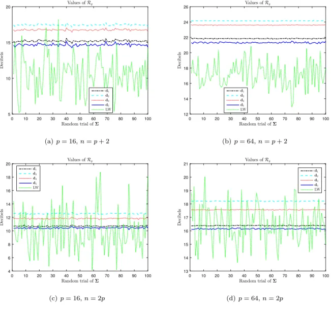
)UT where UFig. 4. Risks of the various estimators over 100 random trials ofΣ. p=64 and n=2p.
is uniformly distributed over the set of unitary matrices, and
λ
jare independent random variables drawn uniformly on]0
,
1]. For eachΣ, the risksRq(Σ, ˆ
Σ) (q=
1−
3,
5) are evaluated for vectors d1, d2, d3anddˆ
5, and for the LW estimator.The results are reported inFigs. 1–2for p
=
16 and inFigs. 3–4for p=
64. These curves show rather interesting results. First note that d1performs well forR5(GΣ,
d) and, vice versa,dˆ
5is very good forR1(Σ,
d). Additionally both ofthem are quite accurate with respect toR3(GΣ
,
d). Therefore, it seems that the new estimatordˆ
5bears some resemblancewith Stein’s initial method. A similarity is also observed between d2and d3which performs well only onR2(GΣ
,
d) and R3(GΣ,
d). As for the LW estimator, it performs very poorly onR2(Σ, ˆ
Σ), poorly onR1(Σ, ˆ
Σ) andR3(Σ, ˆ
Σ) but is thebest method forR5(Σ
, ˆ
Σ), at least when n=
p+
2. For n=
2p, d1anddˆ
5achieve the same risksR1(Σ, ˆ
Σ) andR5(Σ, ˆ
Σ)as the LW estimator. However a striking fact is that the risks associated with the LW estimator are highly variable whenΣ
varies. In contrast, the estimators based on d1−3have constant risksR1−3(GΣ
,
d) and their riskR5(GΣ,
d1−3) varies veryweakly. Similarly,d
ˆ
5offers weakly varying risksR1−3,5(GΣ, ˆ
d5). Therefore, while the LW has often a lower riskR1,5(Σ, ˆ
Σ),it exhibits some instability as the values of the risks are highly dependent onΣ, which is a drawback in practice. To close this section, we now evaluate the respective merits of the above estimates on another loss function, which is highly relevant for the case of interest where covariance matrices are concerned, since it is the (square of the) natural distance between covariance matrices defined as
Lg(Σ
, ˆ
Σ)=
p∑
k=1 log2λ
k(Σ −1Σˆ
) (16)where the
λ
ks are the generalized eigenvalues of (Σˆ
,
Σ). The corresponding risk is defined asRg(Σ, ˆ
Σ)=
E{
Lg(Σ, ˆ
Σ)}
.The loss in (16)corresponds to the natural distance betweenΣand Σ
ˆ
in the set of positive definite matrices (Bhatia,8
Fig. 5. Risk corresponding to the natural distance of the various estimators over 100 random trials ofΣ. p=16 (left panel) and p=64 (right panel).
zero-mean Gaussian distributions with different covariance matrices (Amari et al.,1987;Atkinson and Mitchell,1981). It is thus a very relevant metric and there is interest in comparing d1, d2, d3andd
ˆ
5on this third-party, meaningful criterion.As before, the risks were computed for 100 differentΣ. The results are given inFig. 5. They show that the LW estimator offers the smallest risk, followed byd
ˆ
5, which is the best among estimators based on regularization of the Cholesky factor.Note that the difference betweend
ˆ
5and LW is rather small for n=
2p. Therefore, given thatdˆ
5results in much smallerrisk variability, it constitutes an interesting trade-off.
4. Conclusions
In this paper, we considered estimation of a covariance matrix using Stein’s approach. We focused on estimates of the formΣ
ˆ
=
GSdiag(d)GTS where GSis the Cholesky factor of the sample covariance matrix. This problem was addressedby Stein, Selliah, Eaton and Olkin for various loss functions. We extended this kind of approach to a recently introduced Riemannian metric on the set of lower triangular matrices with positive diagonal elements. The optimal regularization vector was shown to depend onΣbut we proposed an iterative scheme that incurs a very small loss and offers a good trade-off over various loss functions, including the natural distance between covariance matrices. Moreover, the risks associated with this new estimator are very weakly dependent onΣ.
CRediT authorship contribution statement
Olivier Besson: Conceptualization, Methodology, Validation, Software, Writing - original draft, Writing - review &
editing. François Vincent: Conceptualization, Methodology, Validation, Writing - original draft, Writing - review & editing.
Xavier Gendre: Conceptualization, Methodology, Validation, Writing - original draft, Writing - review & editing. References
Amari, S.-I., Barndorff-Nielsen, O.E., Kass, R.E., Lauritzen, S.L., Rao, C.R., 1987. Chapter 5: Differential metrics in probability spaces. In: Gupta, S.S. (Ed.), Differential Geometry in Statistical Inference. In: Lecture Notes–Monograph Series, vol. 10, Institute of Mathematical Statistics, Hayward, CA, pp. 217–240.
Atkinson, C., Mitchell, F.S., 1981. Rao’s distance measure. Sankhya 43 (3), 345–365. Bhatia, R., 2007. Positive Definite Matrices. Princeton University Press.
Chen, Y., Wiesel, A., Eldar, Y.C., Hero, A.O., 2010. Shrinkage algorithms for MMSE covariance estimation. IEEE Trans. Signal Process. 58 (10), 5016–5029. Coluccia, A., 2015. Regularized covariance matrix estimation via empirical Bayes. IEEE Signal Process. Lett. 22 (11), 2127–2131.
Dey, D.K., Srinivasan, C., 1985. Estimation of a covariance matrix under Stein’s loss. Ann. Statist. 13 (4), 1581–1591. Dey, D.K., Srinivasan, C., 1986. Trimmed minimax estimator of a covariance matrix. Ann. Inst. Statist. Math. 38, 101–108. Eaton, M.L., Olkin, I., 1987. Best equivariant estimators of a Cholesky decomposition. Ann. Statist. 15 (4), 1639–1650. Gupta, A.K., Nagar, D.K., 2000. Matrix Variate Distributions. Chapman & Hall/CRC, Boca Raton, FL.
Haff, L.R., 1979. An identity for the Wishart distribution with applications. J. Multivariate Anal. 9, 531–544.
Haff, L.R., 1980. Empirical Bayes estimation of the multivariate normal covariance matrix. Ann. Statist. 8 (3), 586–597.
Ikeda, Y., Kubokawa, T., Srivastava, M.S., 2016. Comparison of linear shrinkage estimators of a large covariance matrix in normal and non-normal distributions. Comput. Statist. Data Anal. 95, 95–108.
James, W., Stein, C., 1992. Estimation with quadratic loss. In: Kotz, S., Johnson, N. (Eds.), Breakthroughs in Statistics. In: Springer Series in Statistics (Perspectives in Statistics), Springer, pp. 443–460.
Konno, Y., 2009. Shrinkage estimators for large covariance matrices in multivariate real and complex normal distributions under an invariant quadratic loss. J. Multivariate Anal. 100 (10), 2237–2253.
Ledoit, O., Wolf, M., 2004. A well-conditioned estimator for large-dimensional covariance matrices. J. Multivariate Anal. 88 (2), 365–411. Ledoit, O., Wolf, M., 2018. Optimal estimation of a large dimensional covariance matrix under Stein’s loss. Bernoulli 24 (4B), 3791–3832. Lin, Z., 2019. Riemannian geometry of symmetric positive definite matrices via Cholesky decomposition. SIAM J. Matrix Anal. Appl. 40 (4), 1353–1370. Lin, S., Perlman, M., 1985. A Monte Carlo comparison of four estimators of a covariance matrix. In: Krishnaiah, P.R. (Ed.), Multivariate Analysis VI.
North Holland, Amsterdam, pp. 411–429.
Ma, T., Jia, L., Su, Y., 2012. A new estimator of covariance matrix. J. Statist. Plann. Inference 142 (2), 529–536. Muirhead, R.J., 1982. Aspects of Multivariate Statistical Theory. John Wiley & Sons, Hoboken, NJ.
Perron, F., 1992. Minimax estimators of a covariance matrix. J. Multivariate Anal. 43 (1), 16–28.
Pourahmadi, M., 2013. High Dimensional Covariance Estimation. In: Wiley Series in Probability and Statistics, John Wiley & Sons, Hoboken, NJ. Scharf, L.L., 1991. Statistical Signal Processing: Detection, Estimation and Time Series Analysis. Addison Wesley, Reading, MA.
Selliah, J.B., 1964. Estimation and Testing Problems in a Wishart Distribution. Technical report no. 10, Department of Statistics, Stanford University. Sheena, Y., 1995. Unbiased estimator of risk for an orthogonally invariant estimator of covariance matrix. J. Japan Statist. Soc. 25 (1), 35–48. Sheena, Y., Takemura, A., 1992. Inadmissibility of non-order preserving orthogonally invariant estimators of the covariance matrix in the case of
Stein’s loss. J. Multivariate Anal. 41, 117–131.
Srivastava, M.S., 2002. Methods of Multivariate Statistics. John Wiley & Sons., New York.
Stein, C., 1956. Inadmissibility of the usual estimator for the mean of a multivariate distribution. In: Proceedings 3rd Berkeley Symposium on Mathematical Statistics and Probability. pp. 197–206.
Stein, C., 1986. Lectures on the theory of estimation of many parameters. J. Math. Sci. 34, 1373–1403.
Tsukuma, H., 2016. Estimation of a high-dimensional covariance matrix with the Stein loss. J. Multivariate Anal. 148, 1–17.
Tsukuma, H., Kubokawa, T., 2016. Unified improvements in estimation of a normal covariance matrix in high and low dimensions. J. Multivariate Anal. 143, 233–248.