Synchronisation, détection et égalisation de modulation à phase continue dans des canaux sélectifs en temps et en fréquence

(1)

En vue de l'obtention du

DOCTORAT DE L'UNIVERSITÉ DE TOULOUSE

Délivré par :

Institut National Polytechnique de Toulouse (Toulouse INP)

Discipline ou spécialité :

Informatique et Télécommunication

Présentée et soutenue par :

M. ROMAIN CHAYOT le mardi 15 janvier 2019

Titre :

Unité de recherche : Ecole doctorale :

Synchronisation, détection et égalisation de modulation à phase continue

dans des canaux sélectifs en temps et en fréquence

Mathématiques, Informatique, Télécommunications de Toulouse (MITT) Institut de Recherche en Informatique de Toulouse (I.R.I.T.)

Directeur(s) de Thèse : M. CHARLY POULLIAT MME MARIE LAURE BOUCHERET

Rapporteurs :

M. DANIEL ROVIRAS, CNAM PARIS M. YVES LOUET, SUPELEC RENNES

Membre(s) du jury :

Mme MARYLINE HELARD, INSA DE RENNES, Président M. CHARLY POULLIAT, INP TOULOUSE, Membre

M. CHRISTOPHE JEGO, UNIVERSITÉ DE BORDEAUX, Membre Mme MARIE LAURE BOUCHERET, INP TOULOUSE, Membre

Mme NATHALIE THOMAS, INP TOULOUSE, Membre

(2)

(3)

Remerciements

Je souhaite remercier en premier lieu toutes les personnes qui, au quotidien, m’ont accom-pagné pendant ces trois années. Votre soutien a beaucoup compté et je vous en remercie chaleureusement.

Merci à mes directeurs de thèse, Charly Poulliat, Marie-Laure Boucheret et Nathalie Thomas pour leurs confiances, leurs encouragements et leurs soutiens au cours de ces années. Sans eux, ce travail ne se serait pas déroulé dans ces conditions quasi-optimal. Merci pour leurs conseils et les discussions qui ont permis de résoudre bien des problèmes auxquelles j’ai été confronté. Merci particulièrement à Charly qui a su me pousser pour réussir, comme tout bon mentor doit savoir faire.

Je tiens également à remercier mes encadrements « industriels » Guy Lesthievent (CNES) et Nicolas Van Wambeke (Thales Alenia Space) pour leur soutien durant la thèse.

Je remercie également toutes les personnes que j’ai pu côtoyer durant ces trois ans au laboratoire TéSA. Les discussions (plus ou moins pertinentes), la pause-café et la bonne ambiance ont été des facteurs déterminants à la réussite de cette thèse. Corinne, Jean-Yves, Philippe, David, Raoul, Patrice (et nos discussions passionnées d’Histoire), Sylvain, Quentin, Julien, Barbara, Selma (la liste est longue), Fabio, Adrien, Lorenzo (aka Chorizo), Isabelle. . . J’arrête la liste-là (puisqu’elle est en réalité bien trop longue) mais sachez que je vous remercie tous pour votre compagnie.

Je tiens particulièrement remercier Charles-Ugo et Simone, mes fidèles camarades de bu-reau, qui m’ont suivi lors de mon déménagement dans la bibliothèque de TéSA. Nos dis-cussions, les blagues et votre bonne humeur me manquent. Ces derniers mois, lors de la préparation de la soutenance, j’ai été accompagné par de nouveaux collègues (et amis) à Thales. Merci à eux pour leur aide dans les répétitions mais également pour leur humour des plus fins et délicats. Puisqu’ils pimentent ma vie en dehors du travail, je remercie également tous mes amis qui ont aussi su m’accompagner durant ces trois ans dans les bons comme dans les mauvais moments.

Pour finir, mes remerciements vont à ma famille, mes sœurs et mes parents qui m’ont toujours soutenu dans mes choix scolaires et de carrière. Je leur dois ce que je suis devenu et je les remercie énormément.

(4)

(5)

List of Figures

1 Lien de commande et contrôle par satellite . . . 2

2 Vue d’ensemble du spectre autour des 5GHz (de [Ben15] . . . 2

3 Signal CPM dans le plan polaire (CPM quaternaire, L=2, h=1/4, RC . . . . 4

4 CNPC by satellite . . . 8

5 Overview of the 5GHz Spectrum (from [Ben15] . . . 8

6 CPM signal in a polar plan (Quaternary CPM, L=2, h=1/4, RC pulse shape 9 1.1 BICM for CPM signals . . . 17

1.2 Overall CPM receiver . . . 17

1.3 Power Spectral Densities for a RC and REC pulse shape CPM schemes, h = 1/3 and L = 2 . . . . 19

1.4 Influence of h on the Power Spectral Density and on the Bit Error Rate . . . 20

1.5 Influence of the CPM memory L on the PSD . . . . 21

1.6 Laurent Representation of a CPM signal . . . 22

1.7 Laurent Pulses for a binary CPM . . . 24

1.8 Trellis using PAM Decomposition . . . 26

1.9 CPM SISO MAP using PAM Decomposition . . . 27

1.10 SISO receiver . . . 30

1.11 EXIT charts for a binary CPM with a RC pulse shape, a memory of L = 2 and h = 1/4 . . . . 31

1.12 SE for 1-REC with different modulation indices . . . 33

1.13 SE for 2-RC with different modulation indices . . . 34

2.1 BICM for CPM with CP or UW insertion . . . 39

2.2 Receiver structure (with CP removal in dotted lines, if CP is used) . . . 39

(8)

2.4 Block-based structure of the CPM signal using a CP . . . 41

2.5 Block-based structure of the CPM signal using a UW . . . 41

2.6 MMSE-FDE of [VT+09] . . . 50

2.7 MMSE-FDE of [PV06] . . . 53

2.8 Periodization of the time-averaged auto-correlation function . . . 57

2.9 Proposed Exact Low-complexity MMSE-FDE . . . 58

2.10 Uncoded BER over general ISI channel . . . 61

2.11 Maximum achievable coding rate for the different MMSE-FDE . . . 62

2.12 BER over frequency-selective channel . . . 63

2.13 Finite impulse responses of hc(t) and h(t) . . . . 64

2.14 Channel estimation MSE over the aeronautical channel . . . 67

2.15 Uncoded BER over the aeronautical channel with channel estimation . . . 68

2.16 BER over aeronautical channel with channel estimation and turbo-detection . 69 2.17 CFO Estimation over AWGN channel . . . 71

2.18 Performance of the carrier recovery . . . 74

2.19 Comparison with the method suited to the AWGN channel . . . 75

2.20 Performance of the carrier recovery with perfect channel knowledge . . . 76

2.21 MSE of the channel estimate . . . 77

2.22 MSE of the channel estimate with perfect carrier recovery . . . 78

2.23 Carrier Recovery for binary CPMs over AWGN channel . . . 82

2.24 Carrier Recovery for 4-ary CPMs over AWGN channel . . . 82

2.25 Carrier Recovery for Binary 3-GMSK h=1/3 over Urban GSM channel . . . . 83

2.26 Carrier Recovery for Binary 2-RCS2 h=1/2 over Urban GSM channel . . . . 83

2.27 Carrier Recovery for Quaternary 3-RC h=1/4 over Urban GSM channel . . . 83

2.28 Carrier Recovery for Quaternary 3-REC h=1/3 over Urban GSM channel . . 84

2.29 Comparison between H&P and random sequence preamble for Quaternary 3-REC h=1/3 over Urban GSM channel . . . 84

(9)

3.1 Transmitter structure with CP or UW insertion . . . 89

3.2 Receiver structure (with CP removal in dotted lines, if CP is used) . . . 89

3.3 Block-based structure of the CPM signal using a UW . . . 90

3.4 Overall Receiver Structure . . . 98

3.5 Influence of the parameter Q . . . . 99

3.6 Influence of the parameter Q and of the number of iteration . . . 100

3.7 Comparison with the LTV-MMSE [Dar+18] . . . 101

3.8 Partitioning of the time-domain channel matrix . . . 107

3.9 NMSE over TIV channels . . . 108

3.10 NMSE over TV channels using KL-BEM . . . 109

3.11 NMSE over TV channels using OCE-BEM . . . 109

3.12 NMSE over TV channels using KL-BEM for block-based CPM . . . 110

3.13 Carrier Recovery for CE-BEM channel . . . 114

3.14 Carrier Recovery for OCE-BEM channel . . . 114

4.1 g0(t) . . . 119

4.2 g1(t) and g1(t) . . . 119

4.3 {gi(t)}, for 2 Æ i Æ 11 . . . 119

4.4 Information Rate for FWD Link . . . 120

4.5 Influence of the size of the packet on the BER for the FWD link . . . 121

4.6 Pulse shapes for the FWD and RTN links . . . 122

4.7 Information Rate for RTN Link . . . 123

4.8 Laurent Pulses for RTN Link . . . 124

4.9 EXIT analysis of the RTN Link CPM concatenated with a (4,[15,17]) convolu-tional code . . . 125

4.10 Influence of the size of the packet on the BER . . . 126

(10)

4.12 CFO Estimation over AWGN channel . . . 128

4.13 Carrier Recovery for FWD and RTN Link over a TIV aeronautical channel . 128 4.14 Carrier Recovery for 4-ary CPMs over AWGN channel . . . 129

4.15 BER over aeronautical channel for the RTN link . . . 129

4.16 BER over aeronautical channel for the FWD link . . . 130

4.17 BER over TV aeronautical channel for the RTN link . . . 130

A.1 SE for h = 1/8 . . . 136

A.2 SE for h = 1/10 . . . 137

B.1 MMSE-FDE with orthogonal representation from [TS05] . . . 141

B.2 MMSE-FDE from [TS05] . . . 145

(11)

List of Tables

1.1 Pulse Shape Table . . . 19

1.2 Duration of the Laurent Pulses . . . 23

2.1 Bandwidth efficiency loss with the UW . . . 42

2.2 Bandwidth efficiency loss with a CP . . . 42

2.3 Relation between the TIV-MMSE-FDE . . . 59

2.4 Computational complexity comparison between the over-sampled MMSE-FDE equalizers . . . 60

4.1 FWD Link parameters . . . 118

4.2 RTN Link parameters . . . 120

(12)

(13)

Table des sigles et acronymes

ASK Amplitude Shift Keying

AWGN Additive White Gaussian Noise

BCJR Bahl, Cocke, Jelinek and Raviv

BEM Basis Expansion Model

BER Bit Error Rate

BICM Bit Interleaved Coded Modulation

CFO Carrier Frequency Offset

CNPC Command and Non Payload Communication

CP Cyclic Prefix

CPM Continuous Phase Modulation

CRB Cramer Rao Bound

DA Data Aided

(I)DFT (Inverse) Discrete Fourier Transform EXIT EXtrinsic Information Transfer

FD Frequency Domain

FIR Finite Impulse Response

FS Fractionally-Spaced

FWD ForWarD Link

GMSK Gaussian Minimum Shift Keying

GPS Global Positionning System

GSM Global System for Mobile Communications

IR Information Rate

LDPC Low Density Parity Check code

LLR Log Likelihood Ratio

(14)

LPF Low Pass Filter

LS Least Squares

LTV Linear Time Varying

MAP Maximum A Posteriori

ML Maximum Likelihood

MSE Mean Square Error

MMSE Minimum Mean Square Error

MMSE-FDE MMSE Frequency Domain Equalizer

OFDM Orthogonal Frequency-Division Multiplexing

PAM Pulse Amplitude Modulation

PSD Power Spectral Density

PSK Phase Shift Keying

RC Raised Cosine

REC RECtangular

RTN ReTurN link

SC-FDE Single Carrier Frequency Domain Equalization

SE Spectral Efficiency

SISO Soft Input Soft Output SNR Signal to Noise Ratio

SOQPSK Shaped Offset Quadrature Phase Shift Keying SVD Singular Value Decomposition

TD Time-Domain

TIV Time InVariant

TV Time Variant

UAV Unmanned Aerial Vehicle

UW Unique Word

(15)

Introduction (Français)

Contexte de la thèse

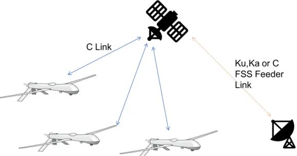
Alors que l’idée des drones (ou UAV pour son acronyme anglais) est apparue au début du siècle dernier avec le premier vol sur 100 kilomètres d’un avion équipé d’un système de pi-lotage automatique, les drones ne sont devenus populaires que depuis une poignée d’années pour des applications nombreuses et diverses. En effet, maintenant, les drones sont considé-rés pour des problématiques de télémesure, d’observation (surveillance des frontières et des forêts, inspections de ponts et de bâtiments), de télédétection, de communications (en cas de catastrophes naturelles par exemple), de divertissement (spectacles nocturnes), de livraison de marchandises, etc. Comme la présence d’un réseau de communication terrestre n’est pas garantie pour de nombreux cas d’usages, un lien de communication par satellite fiabiliserait les communications avec les drones, et particulièrement le lien de commande et contrôle. Enfin, il faut s’assurer de l’intégration complète et sûre des drones dans le trafic aérien actuel.

Pour le moment, les systèmes de communications de drone utilisent la bande KU Fixed Sa-tellite Service (FSS) pour communiquer avec la station au sol à distance (RPS). L’organisation internationale de l’aviation civile (ICAO) et l’Union internationale des télécommunications (ITU ) cherchent à standardiser un système de communications dans la bande C. L’annexe 10 de la Convention de Chicago relative à l’aviation civile internationale porte spécifiquement sur les télécommunications aéronautiques et récemment le Radio Technical Commission for Aeronautics (RTCA) a commencé à développer des exigences et des standards pour le lien de contrôle des drones (Control and Non-Payload Communication CNPC ) avec en premier le lien terrestre [RCT16]. Concernant la couche physique, ils ont proposé une modulation à phase continue, la GMSK (Gaussian Minimum-Shift Keying), à cause de ses propriétés in-téressantes, comme son efficacité énergétique, son occupation spectrale ou sa robustesse au bruit. Ainsi, dans l’optique de réduire l’encombrement des drones, des modulations à phase continue sont également considérées pour le lien satellitaire (comme illustré dans la Figure.1) et nous proposons dans cette thèse d’étudier cette famille de modulations non-linéaires.

L’ITU propose d’utiliser la bande de fréquence des 5030-5091 MHz (la bande C) pour le Aeronautical Mobile en-Route Service (AM(R)S) du lien de contrôle. Ce nouveau lien de communication ne devrait pas interférer avec l’infrastructure déjà en place. La Figure 2 résume les allocations de fréquence autour la bande C.

Dans ce scénario, le signal transmis est sujet à de fortes perturbations dues au canal aéro-nautique par satellite. De plus, à cause du contexte spatial, le signal sera également perturbé par les amplificateurs embarqués travaillant dans des régimes proches de la saturation. Dif-férentes solutions ont été étudiées pour lutter contre ces problèmes comme la pré-distorsion (qui consiste à inverser la fonction de transfert des différentes distorsions), ou l’égalisation du signal à la réception. Des modulations sont par nature robustes à ces non-linéarités comme

(16)

Figure1 – Lien de commande et contrôle par satellite

(17)

les modulations Interplex ou les modulations à phase continue.

Dans ce thèse, nous allons considérer les modulations à phase continue puisque ces derniers présentent des propriétés intéressantes en terme d’occupation spectrale, de consommation énergétique et que leur structure est facilement utilisable dans le cadre d’une concaténation en série avec un code correcteur d’erreur.

Modulation à Phase Continue

Les modulations à phase continue (ou CPM pour Continuous Phase Modulation) sont consi-dérées pour de nombreuses et diverses applications comme les communications avec l’espace lointain (deep space) [Sim05] [Yue06] ou plus récemment pour des applications de télémesure où la modulation SOQPSK (Shaped Offset Quadrature Phase Shift Keying) a été standardisée [IRI17]. Elles ont également été utilisées pour les communication mobiles (GSM) [DCTS97], les communications militaires [CFC10] [CFC10], communications sur ondes millimétriques [DHJ07] [Nse+07] et les communications équipement à équipement (Device to Device) dans la 5G [WGPS11] [Boc+16].

La CPM est une candidate en lice pour le lien de communication d’un drone à un satellite. En effet, son enveloppe complexe constante la rend robuste aux non-linéarités introduites par les amplificateurs embarqués travaillant à un régime saturé et ainsi améliore le bilan de liaison globale puisqu’elle ne nécessite pas de diminuer la puissance en entrée pour les HPA (High Power Amplifiers). De plus, son occupation spectrale est meilleure que celles de certaines modulations linéaires comme les modulations PSK ( Phase Shift Keying), ce qui améliore la capacité du système de communication.

Les signaux CPM ont été grandement étudiés dans le cas de transmission sur des canaux à bruit blanc additif Gaussien (ou AWGN ) et ont montré leur efficacité lors de leur conca-ténation en série avec un code correcteur (comme un code convolutif ou un code LDPC). Si un code LDPC est bien conçu, une CPM concaténée à ce code LDPC peut être proche de la capacité avec une complexité de décodage faible [Ben15].

De façon étonnante, pour des transmissions sur des canaux sélectifs en fréquence, le peu de travaux réalisés montre la difficulté de traiter cette famille de modulations non-linéaires dans ce contexte. [TS05], [PV06] et [VT+09] proposent des égaliseurs dans le domaine fré-quentiel minimisant un critère d’erreur moyenne quadratique (MMSE-FDE pour Minimum Mean Square Error -Frequency-Domain Equalizers (MMSE-FDE)) dans le contexte de trans-missions de signaux CPM sur des canaux sélectifs en fréquence. Cependant, comme montré dans cette thèse, [TS05] repose sur des hypothèses trop restrictives sur le canal de propagation pour en faire un schéma utilisable en pratique tandis que [PV06] et [VT+09] qui proposent deux approches différentes pour égaliser le signal (le premier repose sur la décomposition de Laurent) ont en fait les mêmes performances et sont équivalents (théoriquement prouvé dans [Cha+17a]). Dans les deux cas, ces méthodes par bloc ont une complexité calculatoire importante puisqu’elles requièrent d’inverser des matrix pleines, contrairement aux cas des

(18)

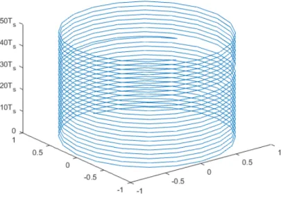
Figure 3 – Signal CPM dans le plan polaire (CPM quaternaire, L=2, h=1/4, RC

modulations linéaires ( Single Carrier Frequency Domain Equalizer SC-FDE).

Les problématiques de synchronisation pour CPM sur canal AWGN ont été étudiées dans [MD97] où plusieurs chapitres lui sont entièrement consacrés. Une étude complète de la syn-chronisation temporelle, fréquentielle et trame pour CPM sur canal AWGN a été conduite au début des années 2010 dans [Hos13] où les bornes théoriques ont également été calculées. Ce-pendant, à notre connaissance, la synchronisation pour signaux CPM tranmis sur des canaux sélectifs en fréquence ou doublement sélectifs n’a pas été étudiée. De plus, l’estimation canal est également une problématique fastidieuse qui a été très peu abordée.

Sans surprise, l’égalisation et la synchronisation pour CPM sur canaux doublement sé-lectifs ont été très étudiées dans des articles comme [Dar+16] pour l’égalisation ou plus récemment [OLS18] pour l’égalisation et une estimation canal aveugle conjointe.

Plan et contibutions principales

Pendant cette thèse, notre objectif a été d’étudier des récepteurs pour modulations à phase continue dans le cas de canaux sélectifs en fréquence ou doublement sélectifs. La principale application est le lien communication des drones par satellite (avec le canal dit aéronautique par satellite). Le plan du manuscrit de thèse et les principales contributions de la thèse sont résumés ci-dessous :

Chapitre 1 : Dans ce chapitre, nous donnons une description des signaux CPM. Nous

(19)

notations utiles pour la suite sont également données. Nous introduisons également une re-présentation en treillis des signaux CPM [Lau86] et décrivons le récepteur associé dans le cas d’une transmission sur canal AWGN [CB05]. Finalement la structure globale d’un récepteur est décrite. Nous donnons également quelques pistes de réflexion sur des méthodes de pré-codage qui permettent soit d’augmenter l’efficacité spectrale [Mes+16] ; [OSL17] soit d’éviter d’itérer entre le détecteur et le code correcteur d’erreur [Per+10].

Chapitre 2 : Ce chapitre traite des transmissions de signaux CPM sur des canaux sélectifs

en fréquence. Nous nous intéressons dans un premier temps à la problématique d’égalisation qui est plus complexe que dans le cas des modulations linéaires. En effet, dans le cas des modu-lations linéaires, nous avons un modèle linéaire gaussien par rapport aux symboles transmis ; ce n’est pas le cas avec les CPM. Cependant, un modèle linéaire Gaussien peut être obtenu par rapport à un vecteur de pseudo-symboles (provenant de la décomposition de Laurent [Lau86]) ou à un vecteur des échantillons de l’enveloppe complexe. Ainsi, dans ce chapitre, nous pré-sentons les principaux égaliseurs de la littérature ([TS05] ; [PV06] ; [VT+09] et montrons leurs différences. Nous présentons également un nouvel égaliseur de faible complexité pour CPM qui est exact (i.e. qui ne fait aucune approximation sur le signal) et qui exploite les propriétés statistiques périodiques du signal dû à sa transmission par bloc étendu circulairement.

Dans un second temps, nous présentons des méthodes d’estimation canal pour CPM qui sont compatibles avec les précédents égaliseurs. De plus, nous développons un estimateur conjoint du canal et de l’erreur de fréquence résiduel (Carrier Frequency Offset) pour CPM, et montrons que sa variance atteint la borne de Cramér Rao Bound.

Les résultats de ce chapitre ont été publiés dans :

• Article de journal : R. Chayot, N. Thomas, C. Poulliat, M.-L. Boucheret, G. Lesthievent, N. Van Wambeke, "A New Exact Low-Complexity MMSE Equalizer for Continuous Phase Modulation", IEEE Communications Letters, 2018

• Article de conférence : R. Chayot, N. Thomas, C. Poulliat, M.-L. Boucheret, N. Van Wambeke, G. Lesthievent, "Channel Estimation and Equalization for CPM with appli-cation for aeronautical communiappli-cations via a satellite link", IEEE Int. Military

Com-munications Conference (MILCOM), Baltimore (MD), U.S.A, 2017

• Article de conférence : R. Chayot, M.-L. Boucheret, C. Poulliat, N. Thomas, N. Van Wambeke, G. Lesthievent, "Joint Channel and Carrier Frequency Estimation for M -ary CPM over frequency-selective channel using PAM decomposition", IEEE Int. Conf.

Acoust., Speech, and Signal Proc. (ICASSP), New Orleans LA, U.S.A, 2017

• Article de conférence : R. Chayot, N. Thomas, C. Poulliat, M.-L. Boucheret, N. Van Wambeke, G. Lesthivent, "Sur l’égalisation fréquentielle des modulations à phase conti-nue", Colloque GRETSI sur le traitement du Signal, Juan-les-pins, France, 2017

Chapitre 3 : Dans ce chapitre, nous nous consacrons au récepteur pour signaux CPM

(20)

signal reçu, nous dérivons un nouvel égaliseur dans le domaine fréquentiel, qui exploite la structure en "bande" de la matrice canal dans le domaine fréquentiel pour réduire sa com-plexité au prix d’une approximation. A notre connaissance, l’égalisation de signaux CPM sur canal doublement-sélectifs a été très peu abordée avec par exemple [Dar+16] qui présente un égaliseur dans le domaine temporel.

Ensuite, nous présentons une méthode pour estimer ce canal doublement-sélectif grâce au Basis Expansion Model. Nous exploitons la structure de la trame du signal pour estimer ce canal et ensuite égaliser le signal reçu. Enfin, une extension de notre précèdent estimateur conjoint du canal et de fréquence est introduit.

Les différents résultats de ce chapitre ont été présentés dans :

• Article de conférence : R. Chayot, N. Thomas, C. Poulliat, M.-L. Boucheret, N. Van Wambeke, G. Lesthievent, "Doubly-Selective Channel Estimation for Continuous Phase Modulation", IEEE Int. Military Communications Conference (MILCOM), Los Angeles (CA), U.S.A, 2018

• Article de conférence : R. Chayot, N. Thomas, C. Poulliat, M.-L. Boucheret, G. Les-thievent, N. Van Wambeke, "A Frequency-Domain Band-MMSE Equalizer for Conti-nuous Phase Modulation over Frequency-Selective Time-Varying Channels", European

Signal Processing Conference (EUSIPCO), Rome, Italy, 2018

Chapitre 4 : Ce chapitre présente le système de communication pour le contexte de

cette thèse, qui est le lien de commande et contrôle des drones par satellite. Dans un premier temps, nous décrivons les schémas de transmissions considérés pour la standardisation et faisons une analyse asymptotique de leurs performances (en donnant également des pistes pour une amélioration future). De plus, nous appliquons les méthodes présentées dans les chapitres précédents (détection, égalisation, estimation de paramètre) pour montrer leurs validités dans le contexte de la thèse.

Conclusion et Perspectives : Pour finir, nous résumons les résultats obtenus de cette

thèse et nous tirons une conclusion sur ces deniers. De plus, nous identifions des pistes de travail pour de futurs travaux dans ce contexte.

(21)

Introduction

Context of the thesis

Even if the idea of Unmanned Aerial Vehicle (UAV ) appears a century ago, with a first 100 kilometers-long flight of a plane with a remote/autonomous pilot system, UAVs became a very popular solution for a wide range of applications only since a few years. Indeed, UAVs are now considered for teledetection, earth observation (forest and border surveillance, buildings and bridges inspections), remote sensing, for communications (in case of natural disasters for instance), for entertainment (nighttime shows), for goods delivery, etc. Since the presence of terrestrial networks is not certain in a lot of those applications, a satellite communication link would ensure the reliability of the communication system with the UAV, and especially of the Command & Control link. Moreover, we have to ensure the complete and safe integration of UAV in the air traffic.

For the moment, UAV communication systems use the Ku-band Fixed Satellite Service (FSS) to communicate with the remote pilot station (RPS). However, the International Civil Aviation Organization (ICAO) and the International Telecommunication Union (ITU ) want to standardize the UAV communication system in the C band. Annex 10 of the Chicago

Convention on International Civil Aviation specifically deals with Aeronautical Telecommu-nications and recently the Radio Technical Commission for Aeronautics (RTCA) started to

de-velop requirements and standards for the Control and Non-Payload Communication (CNPC ) with a terrestrial link [RCT16]. Regarding the physical layer, they proposed a Gaussian Minimum-Shift Keying (GMSK ) modulation, due to its many favorable properties, such as low-power consumption, high spectral efficiency, and noise robustness. Hence, in order to reduce the weight of UAV, Continuous Phase Modulation are also considered for the satellite link (as illustrated in Fig.4) and we will only study this link in this thesis.

The ITU proposes to use the the 5030-5091 MHz frequency band (C-band) especially for the Aeronautical Mobile en-Route Service (AM(R)S) for the CNPC. This new established communication link should not interfere with the existing infrastructure. Figure 5 summarizes the main frequency allocations within the targeted 5GHz band.

The transmitted signal would be subject to strong disturbance due to aeronautical channel by satellite. Furthermore, due to the satellite context, it would also be disturbed when embedded amplifiers are working near saturation. Different solutions can be considered to mitigate this issue as pre-distortion (which consists in inverting the transfer function of the distortions), or counterbalancing those distortions of the received signal by equalizing the signal. Others can also considered modulations schemes which are by nature robust to those non-linearities such as Interplex modulation or Continuous Phase Modulation.

In this thesis, we will consider Continuous Phase Modulation as it offers interesting power and spectral efficiency but also for its structure easily adaptable for serially concatenated

(22)

Figure 4 – CNPC by satellite

(23)

Figure 6 – CPM signal in a polar plan (Quaternary CPM, L=2, h=1/4, RC pulse shape schemes with an outer code.

Continuous Phase Modulation

Continuous Phase Modulation (CPM ) are considered for a lot of different applications such as deep-space communications [Sim05] [Yue06] and more recently for telemetry applications where SOQPSK (Shaped Offset Quadrature Phase Shift Keying) modulation are standardized [IRI17]. They have been used or are currently considered also for mobile communications (GSM) [DCTS97], military communications [CFC10] [CFC10], millimeter communications [DHJ07] [Nse+07] and machine-type communications in 5G [WGPS11] [Boc+16].

CPM is a suitable candidate for the communication link between a satellite and a UAV. Indeed, the constant complex envelop makes them robust to non-linearities introduced by embedded amplifiers working at the saturation regime and therefore improves the overall link budget as it does not require back-off for High Power Amplifiers (HPA). Moreover, it has a better spectral occupancy than linear modulations such as Phase Shift Keying (PSK ) modulation, which will also increase the system capacity.

CPM signals have been well studied for transmission over Additive White Gaussian Noise (AWGN ) channel and also prove to be efficient when used with serially concatenated schemes (a convolutional code or a LPDC code as an outer code for example). If properly designed, a Low-Density Parity-Check (LDPC ) code concatenated with a CPM can be close to the capacity with low decoding complexity [Ben15].

(24)

Surprisingly, for transmission over frequency-selective channels, few papers show that this kind of non-linear modulation are more difficult to handle, compared to linear modulation schemes. [TS05], [PV06] and [VT+09] propose different Minimum Mean Square Error -Frequency-Domain Equalizers (MMSE-FDE) for CPM transmission over frequency-selective channels. However, as we will see in this thesis, [TS05] made some hypothesis on the channel which make its practical interest limited, whereas [PV06] and [VT+09] proposed two different approaches (the first one capitalizes on the Laurent Decomposition) but in fact reached the same performance as shown theoretically and by simulation in [Cha+17a]. In both cases, they proposed block methods requiring an important computational complexity as it does require a full-matrix inversion, unlike the Single Carrier Frequency Domain Equalizer (SC-FDE) for linear modulations.

Synchronization for CPM signals over AWGN channels have been studied in [MD97] where several chapters of this book are dedicated to this family of modulation. A full study of timing, carrier and frame synchronization for CPM over AWGN channel has been carried out in 2012 in [Hos13] where also theoretical bounds are derived. But, to our knowledge, the case of a transmission over frequency-selective or doubly-selective channels has not been considered for the synchronization. Moreover, channel estimation is also a tedious issue which has not been well studied.

With no genuine surprise, equalization and synchronization for a CPM transmission over a doubly-selective channel have been studied in a very few papers such as [Dar+16] for equalization or [OLS18] for joint equalization and blind channel estimation.

Dissertation outline and main contributions

In this thesis, we aim to study different receiver techniques for Continuous Phase Modulation over frequency-selective and doubly-selective channels. The main application will be the aeronautical channel for UAV communications by satellite. The dissertation outline and the main contributions are summarized bellow:

Chapter 1: In this chapter, we give an introduction to CPM signals. We define its

main parameters, show their influences on the signal and also give some notations. We also introduce a trellis representation of the CPM signals [Lau86], and its associated detector [CB05] for a transmission over an AWGN channel, to finally describe the overall receiver structure. We give some clues about how to use precoding to enhance the Spectral Efficiency of legacy CPM scheme [Mes+16]; [OSL17] and also how to avoid turbo-detection/decoding [Per+10] in case of serially concatenated CPM schemes.

Chapter 2: This chapter deals with CPM transmissions over frequency-selective channels

(also called time-invariant channels). We will first address channel equalization, which is a little more tedious than for the linear modulation case. Indeed, if in the case of linear modulation, we have a Gaussian linear model of the received signal regarding the transmitted data symbols, this is not the case for CPM signals. However, we do have a Gaussian linear

(25)

model of the received signal with respect to a vector of pseudo-symbols (coming from the Laurent decomposition [Lau86]) or to a vector of collected samples of the received complex envelop. Hence, in this chapter, we will present the main equalizers from the literature ([TS05]; [PV06]; [VT+09] and point out their similitude and differences. We will also present a new exact low-complexity equalizer for CPM which exploits the periodic statistics of the signal in case of circular-extended block-based transmissions.

In a second time, we will present some channel estimation methods for CPM which are compatible with the latter equalizers. We will also present a joint channel and carrier fre-quency estimation for CPM, and show that the variance achieves the derived Cramér Rao Bound (CRB).

The results of this chapter are published in:

• Journal: R. Chayot, N. Thomas, C. Poulliat, M.-L. Boucheret, G. Lesthievent, N. Van Wambeke, "A New Exact Low-Complexity MMSE Equalizer for Continuous Phase Modulation", IEEE Communications Letters, 2018

• Paper: R. Chayot, N. Thomas, C. Poulliat, M.-L. Boucheret, N. Van Wambeke, G. Lesthievent, "Channel Estimation and Equalization for CPM with application for aero-nautical communications via a satellite link", IEEE Int. Military Communications

Con-ference (MILCOM), Baltimore (MD), U.S.A, 2017

• Paper: R. Chayot, M.-L. Boucheret, C. Poulliat, N. Thomas, N. Van Wambeke, G. Lesthievent, "Joint Channel and Carrier Frequency Estimation for M -ary CPM over frequency-selective channel using PAM decomposition", IEEE Int. Conf. Acoust.,

Speech, and Signal Proc. (ICASSP), New Orleans LA, U.S.A, 2017

• Paper: R. Chayot, N. Thomas, C. Poulliat, M.-L. Boucheret, N. Van Wambeke, G. Lesthivent, "Sur l’égalisation fréquentielle des modulations à phase continue", Colloque

GRETSI sur le traitement du Signal, Juan-les-pins, France, 2017

Chapter 3: In this chapter, we will oversee receivers techniques for CPM transmission

over doubly-selective channels. First, after a short presentation of the system model, we will derive an approximate frequency-domain equalizer for CPM over doubly-selective channels, which exploits the band structure of the channel matrix in the frequency-domain to reduce its computational complexity. To our knowledge, only a few equalizers consider the case of doubly-selective channels such as the one in [Dar+16] which is in the Time-Domain.

Then, we will also present how to estimate a doubly-selective channel using the well-known Basis Expansion Model. We will use the particular block-based structure of our CPM transmission to perform such channel estimation and then equalize the received signal. Last, an extension of our previous joint channel and carrier frequency estimation for CPM over doubly-selective channels will be introduced.

(26)

• Paper: R. Chayot, N. Thomas, C. Poulliat, M.-L. Boucheret, N. Van Wambeke, G. Lesthievent, "Doubly-Selective Channel Estimation for Continuous Phase Modulation",

IEEE Int. Military Communications Conference (MILCOM), Los Angeles (CA), U.S.A,

2018

• Paper: R. Chayot, N. Thomas, C. Poulliat, M.-L. Boucheret, G. Lesthievent, N. Van Wambeke, "A Frequency-Domain Band-MMSE Equalizer for Continuous Phase Mod-ulation over Frequency-Selective Time-Varying Channels", European Signal Processing

Conference (EUSIPCO), Rome, Italy, 2018

Chapter 4: This chapter presents the system for the context of this thesis, which is the

CNPC of UAV using a satellite communication link. We will first present the transmission schemes which are currently considered for standardization and also provide an asymptotic analysis of those links (giving some clues on their improvements). Also, we will assess our proposed methods (detection, channel equalization and parameters estimation) in order to show their validity in such contexts.

Conclusion and Perspective: Finally we summarize the main results of this thesis and

(27)

List of publications

Journal Papers

1. R. Chayot, N. Thomas, C. Poulliat, M.-L. Boucheret, G. Lesthievent, N. Van Wambeke, "A New Exact Low-Complexity MMSE Equalizer for Continuous Phase Modulation",

IEEE Communications Letters, 2018

International conference papers

2. R. Chayot, N. Thomas, C. Poulliat, M.-L. Boucheret, N. Van Wambeke, G. Lesthievent, "Doubly-Selective Channel Estimation for Continuous Phase Modulation", IEEE Int.

Military Communications Conference (MILCOM), Los Angeles (CA), U.S.A, 2018

3. R. Chayot, N. Thomas, C. Poulliat, M.-L. Boucheret, G. Lesthievent, N. Van Wambeke, "A Frequency-Domain Band-MMSE Equalizer for Continuous Phase Modulation over Frequency-Selective Time-Varying Channels", European Signal Processing Conference

(EUSIPCO), Rome, Italy, 2018

4. R. Chayot, N. Thomas, C. Poulliat, M.-L. Boucheret, N. Van Wambeke, G. Lesthievent, "Channel Estimation and Equalization for CPM with application for aeronautical com-munications via a satellite link", IEEE Int. Military Comcom-munications Conference

(MIL-COM), Baltimore (MD), U.S.A, 2017

5. R. Chayot, M.-L. Boucheret, C. Poulliat, N. Thomas, N. Van Wambeke, G. Lesthievent, "Joint Channel and Carrier Frequency Estimation for M -ary CPM over frequency-selective channel using PAM decomposition", IEEE Int. Conf. Acoust., Speech, and

Signal Proc. (ICASSP), New Orleans LA, U.S.A, 2017

National conference papers

6. R. Chayot, N. Thomas, C. Poulliat, M.-L. Boucheret, N. Van Wambeke, G. Lesthivent, "Sur l’égalisation fréquentielle des modulations à phase continue", Colloque GRETSI

(28)

(29)

Chapter 1

Communication systems using

CPM Signals

Contents

1.1 Introduction . . . . 16 1.2 Communication systems for CPM over AWGN channels . . . . 17

1.2.1 CPM transmitter . . . 17 1.2.2 Receiver Structure . . . 17

1.3 CPM signals . . . . 18

1.3.1 Definition of CPM signals . . . 18 1.3.2 PAM Representation . . . 20 1.3.3 Symbol-wise MAP detection . . . 25 1.3.4 EXIT Charts and asymptotic analysis . . . 29

1.4 Precoded CPM . . . . 32

1.4.1 CPM with duo-binary encoder . . . 32 1.4.2 Pragmatic CPM . . . 34

Résumé

Dans ce chapitre, nous donnons une description rapide des Modulations à Phase Continue (CPM ). Les modulations à phase continue sont une classe de modulation non linéaire qui a la particularité d’avoir une enveloppe complexe constante, les rendant robustes aux non-linéarités comme celles introduites par les amplificateurs embarqués. De plus, les signaux CPM ont généralement un lobe spectral principal plus étroit que les modulations linéaires de type PSK (Phase Shift Keying). Pour les CPM, les symboles de données sont filtrés par une fonction de mise en forme de la phase assurant la continuité de cette dernière.

Le nom de modulation à phase continue a été introduit dans les papiers fondateurs [ARS81a] [ARS81b] de Tor Aulin, sous la supervision de Carl-Erik Sundberg où une étude théorique de ces signaux a été réalisée et leur structure en treillis exhibée. Cependant, les premières CPM sont apparues avant dans les années 70 avec les modulations Minimum Shift Keying (MSK ) et Frequency Shift Keying (FSK ).

(30)

Les signaux CPM sont envisagés pour de nombreuses applications comme les commu-nications militaires [CFC10], les commucommu-nications à 60Ghz [Nse+07], l’Internet des Objets [DL12], la télémesure aéronautique [Ran15] [IRI17] ou encore les communications aéronau-tiques [RCT16].

Dans un premier temps, nous donnons une définition des signaux CPM et exposons leurs paramètres et leurs influences sur le signal émis. Ensuite, nous décrivons les récepteurs asso-ciés de type Maximum A Posteriori (MAP) aux signaux CPM dans le cas d’une transmission sur canal AWGN utilisant la décomposition de Laurent, qui permet d’écrire un signal CPM comme la somme de modulations PAM modulés par des pseudo-symboles (corrélés et ayant une relation non-linéaire entre eux). Nous en profitons également pour montrer comment cette décomposition peut être utilisée pour calculer la fonction d’auto-corrélation d’un signal CPM. Enfin, nous présentons deux techniques de pré-codage qui permettent soit d’améliorer l’efficacité spectrale d’un schéma considéré soit de rendre inutile les itérations entre code correcteur d’erreur et détecteur CPM.

1.1 Introduction

Continuous Phase Modulation (CPM ) signals are a class of non-linear modulations which have the property of having a constant complex envelop, making them robust to non-linearities such as the ones introduced by embedded amplifiers. For CPM signals, the data symbols are filtered by a phase shaping function which ensures continuous phase from one symbol to another.

The name Continuous Phase Modulation has been introduced in the two seminal papers [ARS81a] [ARS81b] where Tor Aulin, under the supervision of Carl-Erik Sundberg, finalized the theoretical study of CPM signals and of their underlying trellis representations. However, the first CPM system traces back to the 70’s with the Minimum Shift Keying (MSK ) and Frequency Shift Keying (FSK ) modulations. Later, by exploiting the trellis structure of those two modulations, and with the objective of improving the euclidean distance properties, the Continuous Phase Frequency Shift Keying (CPFSK ) has been introduced, which consists of a different modulation index.

CPM signals are considered for a lot of applications such as military communications [CFC10], 60Ghz communications [Nse+07], Internet of Things [DL12], aeronautical teleme-try [Ran15] [IRI17] and also aeronautical communications [RCT16]. Indeed, their constant envelop made them suitable to transmissions through non-linear channels where the ampli-tude of the signal is distorted. Moreover, as the phase transition are continuous, CPM signals benefit from a narrow spectral main lobe (compared to Phase Shift Keying (PSK ) linear modulations).

Last, as we will show in this chapter, their Markov structure makes them suitable for serially concatenated schemes. Several works were conducted on serial concatenated schemes with convolutional codes or other short block codes (see [AAS13] [AS06] and [MA01]). More

(31)

Figure 1.1 – BICM for CPM signals

Figure 1.2 – Overall CPM receiver

recently, [Ben15] proposed the asymptotic analysis and the design of turbo-CPM systems based on the optimization of sparse graph-based codes.

1.2 Communication systems for CPM over AWGN channels

1.2.1 CPM transmitter

In this thesis, we will consider a Bit Interleaved Coded Modulation (BICM ) for CPM, as illustrated in Fig.1.1. At the transmitter side, a binary message b of length K is encoded to a codeword c of length Nc using a error correcting code of rate R = K/Nc and, after being

interleaved, sent to a M-ary mapper to obtain a sequence α œ {±1, ±3, . . . , ±(M ≠ 1)}N_.

This data symbols sequence is then given to the CPM modulator. The transmitted complex envelop of the CPM signals is described in Section 1.3.

1.2.2 Receiver Structure

In this chapter, we only consider a transmission over an AWGN channel and perfect synchro-nization is assumed (Phase noise is not included ; carrier frequency offset, time offset and Doppler spread are not considered either). Hence, at the receiver side, the complex envelope of the received signal is:

r(t) = sb(t) + w(t) (1.1)

where w(t) is a complex white gaussian noise with two-sided power spectral density 2N0.

(32)

we perform Soft Input-Soft Output (SISO) channel decoding, based on the BCJR algorithm [Bah+74]. If iterative turbo detection is used, iterations are performed on extrinsic log like-lihood ratio between the CPM detection and the channel decoder. As we will show, later in Section 1.3.4, in most legacy CPM schemes, turbo-detection is mandatory to avoid any loss of performance and to achieve code capacity. The overall receiver is illustrated in Fig.1.2.

1.3 CPM signals

1.3.1 Definition of CPM signals

Let α = {–n}0ÆnÆN ≠1 œ {±1, ±3, . . . , ±M ≠ 1}N be a sequence of N symbols taken from a

M-ary alphabet . The complex envelope sb(t) associated with the transmitted CPM signal is

written as follows sb(t) = Û 2Es Ts exp (j◊(t, α)) (1.2) where ◊(t, α) = 2ﬁh N ≠1_ÿ i=0 –iq(t ≠ iTs) and q(t) = Y ] [ st 0g(· )d·, t Æ LTs 1/2, t > LTs

Esis the symbol energy, Ts is the symbol period, ◊(t, α) is the information phase, g(t) is the

pulse response, h is the modulation index and L is the CPM memory.

All those parameters and how they affect the CPM properties are discussed in the follow-ing.

1.3.1.1 The Pulse Response q(t)

The pulse response is defined as the primitive function of the frequency pulse g(t): and

q(t) = Y ] [ st 0g(· )d·, t Æ LTs 1/2, t > LTs

It ensures the continuity of the modulation phase as it defines the shape of the phase tra-jectory. Different shapes have been studied since several years allowing the signal to achieve different properties. We choose to focus on different shapes: Raised Cosine (RC ) Shape,

(33)

Name Frequency Pulse Support Parameters REC g(t) = _2LT1 s [0, LTs] L RC g(t) = _2LT1 s(1 ≠ cos( 2ﬁt LTs)) [0, LTs] L

Mixed RC-REC (1 ≠ –)gREC(t) + –gRC(t) [0, LTs] L, –

GMSK g(t) = _LT1 s Ó Q(2ﬁBt≠T_Ô s/2 ln(2)) ≠ Q(2ﬁB t+Ts/2 Ô ln(2)) Ô Infinite L, 0 < BTs< 1

Table 1.1 – Pulse Shape Table

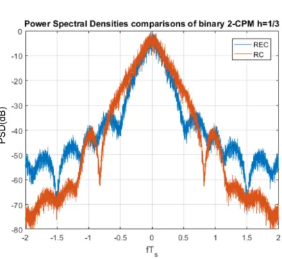
Figure 1.3 – Power Spectral Densities for a RC and REC pulse shape CPM schemes, h = 1/3 and L = 2

Rectangular (REC ) Shape, Mixed Raised Cosine and Rectangular (Mixed RC-REC ) shape and the Gaussian Minimum Shift Keying (GMSK ) shape. Table 1.1 defines those commonly used shapes.

As illustrated in Fig.1.3 where the Power Spectral Densities (PSD) are plotted, the REC pulse shape has a narrower main lobe compared to the RC pulse shape, but it has a greater out-of-band power leakage.

1.3.1.2 The Modulation Index h

This a real number, usually smaller than 1. Generally, it is a constant although in CPM schemes known as multi-h CPM [PT87], it can change cyclically during the transmission (multi-h CPM signals are out of the scope of this thesis). h can also take irrational values, but it leads to a high complexity receiver and then it is not the case in most legacy CPM

(34)

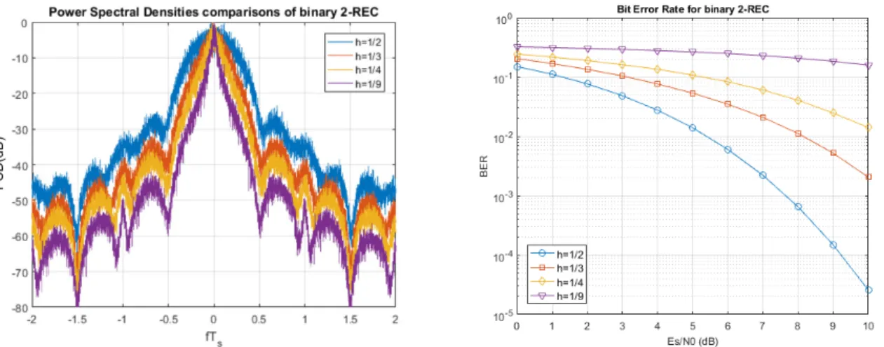
Figure 1.4 – Influence of h on the Power Spectral Density and on the Bit Error Rate schemes.

A smaller h results in a narrower occupied bandwidth, but at the price of a smaller minimal distance as illustrated in Fig.1.4. Generally, h is a rational number such as h =k

p.

1.3.1.3 The CPM Memory L

The CPM Memory L is defined as the support length of g(t). It is also the size of the memory associated to the trellis representation of a CPM signal. In the case where L = 1, CPM signals are called total response CPMs. For instance, Continuous-Phase Frequency-Shift Keying (CPFSK ) modulation and Minimum-Frequency-Shift Keying (MSK ) modulation are total response CPMs.

In the case where L > 1, we refer to partial response CPMs, as the one defined in the DVB-RCS2 standard or the ones considered for standardization for the UAV communication link by satellite.

As L increases, the spectrum occupancy decreases. However, it will increase complexity for the CPM detection as shown latter.

1.3.2 PAM Representation

CPM signals are a non-linear modulation scheme with memory. Hence, it can be represented as a finite-state machine. This structure implies the existence of a trellis representation of the CPM signal. First, [ARS81b] has proposed a time-variant trellis with a number of states that depends on the modulation index. To simplify this structure, [Rim88] introduced a time-invariant trellis. Its associated receiver is composed of a bank of pML _{filters and a non-linear}

(35)

Figure 1.5 – Influence of the CPM memory L on the PSD

CPM schemes serially concatenated with an outer channel coder. However, in the literature, low-complexity CPM detectors have been developed [Kal89] [CB05] by capitalizing on the Laurent Decomposition.

The Laurent Decomposition has been introduced in [Lau86] for binary CPM signals with non-integer modulation index. This decomposition allows us to write the CPM signal as a sum of modulated PAM, where the non-linearity is within the complex pseudo-symbols dependency. In this section, we will present this decomposition and exhibits the underlying trellis structure of the CPM signal.

For more details on the influence of the parameters, readers may refer to [AAS13] and [Cha+04].

1.3.2.1 Derivation

We recall that a CPM signal is given in Eq.(1.2). In this part, we only consider binary CPMs with non-integer modulation index. Using the Laurent Decomposition, the complex baseband signal sb(t) can be expressed as the sum of K = 2L≠1 pulse amplitude-modulated

(36)

Figure 1.6 – Laurent Representation of a CPM signal signals (PAM ), modulated by complex pseudo-symbols ak,n:

sb(t) = K≠1_ÿ k=0 N ≠1_ÿ n=0 ak,ngk(t ≠ nTs) (1.3) gk(t) = s0(t) L≠1_Ÿ j=1 sj+L—k,j(t), 0 < k Æ K ≠ 1 ak,n = ej2fihAk,n Ak,n = n ÿ i=0 –i≠ L≠1_ÿ j=1 –n≠j—k,j sj(t) = sin(Â(t + jT_sin(hfi) s)) Â(t) = Y _ ] _ [ 2fihq(t), 0 Æ t Æ LTs fih ≠ 2fihq(t ≠ LTs), LTsÆ t Æ 2LTs 0, elsewhere (1.4) where —k,j refers to the jth bit in the binary representation of k, k œ 0, 1, . . . , K ≠ 1:

k =

L≠1_ÿ j=1

—k,j2j≠1

Using this representation, a CPM signal can be seen as a sum of linear modulations with correlated pseudo-symbols as shown in Fig.1.6. The K Laurent Pulses {gk(t)}0ÆkÆK≠1 have

different duration lengths by construction, as reported in Table 1.2.

An example of the Laurent Pulses (LP) is given in Fig.1.7 for a binary CPM with a RC pulse shape, h = 1/2 and a memory L = 3. This CPM signals can be represented by four pulses.

As we can see in Fig.1.7, by considering only the first LP which contains most of the energy, a rather good approximation of binary CPM signals with non-integer modulation

(37)

Laurent Pulse Duration g0(t) (L + 1)Ts g1(t) (L ≠ 1)Ts g2(t),g3(t) (L ≠ 2)Ts ... ... g_K/2, . . . , gK≠1 Ts

Table 1.2 – Duration of the Laurent Pulses

index is obtained: sb(t) ¥ N ≠1_ÿ n=0 a0,ng0(t ≠ nTs) (1.5) a0,n= ej2ﬁh qn i=0–i

This properties is often used for CPM detection as it allows to design low-complexity receivers without a noticeable loss of performance.

Extension of the Laurent Decomposition The Laurent decomposition only considers

the case of binary CPM with non-integer modulation index. [MM95] extends this decompo-sition to M-ary CPM, by writing a M-ary CPM signal as a product of binary CPM signals and by applying the Laurent Decomposition on them. Indeed, in this case, a symbol from the

M -ary alphabet {±1, ±3, . . . , ±(M ≠ 1)} is written as –i =qP ≠1p=0 2pbpi with {b p

i}p œ {±1}P

and P = log₂(M). Therefore, the transmitted CPM signal is given by:

sb(t) = exp{fih N ≠1_ÿ i=0 –iq(t ≠ iT )} (1.6) = exp)fih N ≠1_ÿ i=0 ( P ≠1_ÿ p=0 2p_bp i)q(t ≠ iT ) * _(1.7) = P ≠1_ÿ p=0 exp)fih2pbp_i_{q(t ≠ iT )}* (1.8) = P ≠1_ÿ p=0 sbin(t; bp, q, 2ph) (1.9)

where sbin(t; bp, q, 2ph) is a binary CPM with the pulse shape q(.), an index modulation 2ph

and a binary input sequence {bp

i}0ÆiÆN ≠1. The Laurent decomposition is applied on those

binary CPM signals to obtain the PAM decomposition of the M-ary CPM signal.

Also [HL03] extends this work for CPM signals with integer modulation index. [PR05] presents the PAM decomposition for multi-h CPM schemes. In this thesis, we will refer to all those decomposition as the PAM Decomposition of a CPM signal.

(38)

Figure 1.7 – Laurent Pulses for a binary CPM

1.3.2.2 Trellis Representation

[Kal89] exhibited the trellis structure of the Laurent Decomposition. Indeed, let us recall that: Ak,n= n ÿ i=0 –i≠ L≠1_ÿ j=1 –n≠j—k,j (1.10) = A0,n≠1+ –n≠ L≠1_ÿ j=1 –n≠j—k,j (1.11)

Hence, at each nTs, the pseudo-symbols can be computed from the input symbols –nand the

tuples {A0,n≠1, –n≠L+1, –n≠L+2, . . . , –n≠1}.

Hence, the trellis is given by the state ‡n= {A0,n≠1, –n≠L+1, –n≠L+2, . . . , –n≠1} and the

next state is ‡n+1= {A0,n= A0,n≠1+ –n, –n≠L+2, –n≠L+3, . . . , –n}.

By using the approximation where only the first Laurent Pulse is considered, the current state is further reduced to ‡n= {A0,n≠1}, which will be exploited to reduce the computational

(39)

complexity of the detection.

1.3.2.3 Time-averaged auto-correlation function

An other useful tool provided by this Laurent Decomposition is the computation of the time-averaged auto-correlation function of the CPM signals. Indeed, this auto-correlation function is used later in this manuscript when MMSE equalizers are derived in Chapters 2 and 3.

For a time lag ·, the auto-correlation function is defined as

R(· ) = K≠1_ÿ i=0 K≠1_ÿ j=0 Œ ÿ p=≠Œ E_ijpCij(· ≠ pTs) (1.12)

where Cij(◊) is the inter-correlation of the Laurent Pulses given by

Cij(◊) =

⁄

gi(t)gj(t + ·)dt (1.13)

and Ep

ij is the inter-correlation of the complex pseudo-symbols given by

E_ijp = C∆(i,j,p) _(1.14)

and C = cos(hﬁ) (1.15)

∆(i, j, p) is the number of terms in the algebraic expressions of Ai,n≠ Aj,n+p. The

compu-tation of this term is tedious, and therefore we invite the readers to refer to [Lau86] (Eq.526, pp.155) for the details.

One case of interest is when h = 1/2 as in this case C = 0. Therefore, the time-averaged auto-correlation function becomes:

R(· ) =

I qK≠1

k=0 Cii(·) for 0 Æ |·| Æ (L + 1)T

0 elsewhere (1.16)

Others papers deal with the auto-correlation function of CPM signals. [NS01] derives its own decomposition in order to compute high-order statistics of CPM signals including the time-averaged auto-correlation function. [Dar+17] considers an one-sided CPM signal to derive a closed-form function of the time-averaged auto-correlation and cyclic auto-correlation functions.

1.3.3 Symbol-wise MAP detection

As there is no linear relation between the received signal and the data symbols, we need to use a non-linear detector to retrieve them. As we have presented a trellis-based representation of

(40)

CPM signals, we are interested here in trellis-based decoders: the Viterbi algorithm [Vit67] and the BCJR algorithm [Bah+74] are two main representatives of such receivers. The Viterbi algorithm is a Maximum Likelihood Sequence Estimator (MLSE) which means that it outputs the most likely sequence of data symbols whereas the BCJR is a bit/symbol-wise algorithm which produces a Maximum A Posteriori (MAP) probability for each symbols/bits given the whole observation sequence. [Kal89] presents a MLSE and, capitalizing on the Laurent Decomposition, designs a low-complexity detector by taking into account the main Laurent Pulse. Using the metric issued from the MLSE, [CB05] presents a soft MAP detector for CPM over an AWGN channel and also designs a low-complexity receiver by taking into account the main components of the PAM representation.

In this section, we will present the soft MAP decoder of [CB05] as, at the receiver, we are interested in performing turbo-decoding. This MAP decoder capitalizes on the trellis structure resulting from the PAM representation of the CPM signal.

To develop this detector, we have to consider a transmission over an AWGN channel. Therefore, the received signal is given by:

r(t) = sb(t) + w(t) (1.17)

Let us consider the compact representation of the observation, resulting from the PAM de-composition, and represented in Fig.1.8.

Figure 1.8 – Trellis using PAM Decomposition

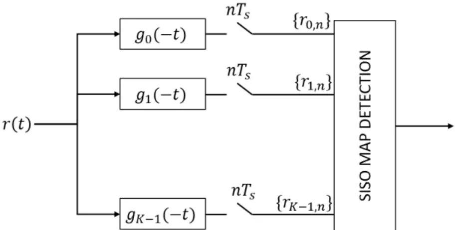
The overall structure of the SISO MAP detector using the PAM Decomposition is given in Fig.1.9 where rk,n is the output of the matched filter to the kth component of the Laurent

Decomposition sampled at nTsand {rk,n}k,n and proven to be sufficient statistics to estimate

the data symbols α. They are given by:

rk,n =

⁄ (L+1)Ts

0

r(t + nTs)gkú(≠t)dt (1.18)

The MAP criterion for the bit –n is given by:

‚ –n= argmax –n p(–n|{rk,n}k,n) (1.19) = argmax –n p(–n; {rk,n}k,n) (1.20) p(–n; {rk,n}k,n) = ÿ Sαn p(‡n≠1= sn≠1, ‡n= sn, {rk,n}k,n) (1.21)

where S–n is the set of transition corresponding to the symbols –n, i.e.

(41)

Figure 1.9 – CPM SISO MAP using PAM Decomposition Let us denote rm

l a set of the sufficient statistics such as

rm_l = [{rk,l}0ÆkÆK≠1, {rk,l+1}0ÆkÆK≠1, . . . , {rk,m}0ÆkÆK≠1] and rn= {rk,n}0ÆkÆK≠1 P = p(‡n≠1= sn≠1, ‡n= sn, {rk,n}k,n) (1.22) = p(‡n≠1= sn≠1, ‡n= sn, rn≠10 , rn, rn+1N ≠1) = p(rN ≠1 n+1|‡n≠1= sn≠1, ‡n= sn, rn≠10 , rn)p(‡n≠1= sn≠1, ‡n= sn, rn≠10 , rn) = p(rN ≠1 n+1|‡n≠1= sn≠1, ‡n= sn, rn≠10 , rn)p(‡n= sn, rn|‡n≠1= sn≠1, r0n≠1)p(‡n≠1= sn≠1, r0n≠1) = p(rN ≠1 n+1|‡n= sn)p(‡n= sn, rn|‡n≠1= sn≠1)p(‡n≠1= sn≠1, rn≠10 ) = p(rN ≠1 n+1|‡n= sn)p(‡n= sn, rn|‡n≠1= sn≠1)p(rn|‡n≠1 = sn≠1, ‡n= sn)p(‡n≠1= sn≠1, r0n≠1) = p(rN ≠1 n+1|‡n= sn)p(‡n= sn, rn|‡n≠1= sn≠1)p(‡n≠1= sn≠1, rn≠10 ) (1.23)

In Eq.(1.23), we can see three terms:

• p(‡n≠1 = sn≠1, rn≠10 ) which only depends on the previous channel observations. This

metric is referred to as the forward metric, and will be denoted as An(sn≠1);

• p(rn+1N ≠1|‡n= sn) which only depends on the future observation. This one is referred to

as the backward metric, and will be denoted as Bn(sn);

• p(‡n = sn, rn|‡n≠1 = sn≠1) is the transition metric, which depends on the current

channel observation and on the a priori probability of the symbol –n. It will be denoted

as Gn(sn≠1, sn).

The transition metric for the AWGN channel can be shown to be proportional to Gn(sn≠1, sn) Ã exp I 2 N0Ÿ )K≠1ÿ k=0 rk,naúk,n *2J ﬁ(–n) (1.24)

(42)

The a priori probability of a symbol can be computed straightforwardly from the a priori probability of the bits if considered independent as in BICM systems. Indeed, by considering a symbol from a M-ary alphabet such as –n = qP ≠1p=0 2pbpn , where {bpi}p œ {±1}P and

P = log₂(M), the probability of this symbol is equal to the product of the probability of its

bits if considered independent as in BICM systems.

The forward and backward metrics can be computed recursively such as: An(s) = ÿ sÕ Gn(sÕ, s)An≠1(sÕ) (1.25) Bn≠1(s) = ÿ sÕ Gn(s, sÕ)Bn(s) (1.26)

The last step of our detector is to compute the extrinsic probability of a bit from the previous a posteriori probability of a symbol. To do so, we have to first compute the a

posteriori probability of each bits from the a posteriori probability (APP) of the symbols.

Let us consider that a symbol from a M-ary alphabet can be written as:

–n= P ≠1_ÿ p=0 2p_bp n (1.27) with {bp i}p œ {±1}P and P = log2(M). Let define by S_b+

p (resp. Sb≠p) the set of symbols where the p

th_{bit is equal to 1 (resp. ≠1),}

i.e. bp

n= +1 (resp. bpn= ≠1 ). The a posteriori probability (APP) of this bit is given by:

p(bp_n= +1; {r_k,n_}k,n) = ÿ S_b+ p p(–n; {rk,n}k,n) (1.28) p(bp_n= ≠1; {r_k,n_}k,n) = ÿ S_b≠ p p(–n; {rk,n}k,n) (1.29)

Then the log-likelihood ratio (llr) of the APP is defined as: llrAPP(bpn) = log A p(bp_n= +1; {r_k,n_}k,n) p(bpn= ≠1; {rk,n}k,n) B (1.30)

The extrinsic llr is obtained by removing the a priori llr (denoted as llra(bpn)):

llrext(bpn) = llrAPP(bpn) ≠ llra(bpn) (1.31) where llra(bpn) = log 3_ﬁ(bp n= +1) ﬁ(bpn= ≠1) 4 (1.32)

(43)

with ﬁ(.) corresponds to the bit a priori probability.

In order to avoid numerical issues as the absolute values of the different metrics can grow to infinity quickly, we use the BCJR algorithm in the log domain by defining the following:

Â Gn(sn≠1, sn) = log(Gn(sn≠1, sn)) Â An(s) = log(An(s)) = maxú sÕ(GÂn(sÕ, s)AÂn≠1(sÕ)) and_BÂ_n≠1(s) = log(Bn≠1(s)) = maxú sÕ(GÂn(s, sÕ)BÂn(s))

where the operator maxú _is:

maxú_{(a, b) = max(a, b) + log(1 + e}≠|a≠b|₎ _(1.33)

To further reduce the complexity of the algorithm, one can use a look-up table to ap-proximate the log part of the operator. Others can also replaced this operator by the max operation at the prize of a slight performance loss.

The main advantage of those receivers is that we can easily reduce their computational complexity. Indeed, as explained in Section 1.3.2.2, binary CPM with non-integer modulation index can be well-approximated by only the first Laurent Pulse, therefore the branch metric in Eq.(1.24) becomes: Gn(sn≠1, sn) Ã exp ; ₂ N0Ÿ ) r0,naú0,n *< ﬁ(–n) (1.34) (1.35) where the trellis state is reduced to ‡n= {a0,n≠1}.

In this thesis, we only consider this soft MAP decoder in the log domain for simulations. However, our results concerning equalization or parameters estimation do not depend on the used CPM detector (Laurent-based or Rimoldi-based). A complete study of the soft MAP detection using the Rimoldi decomposition and the Laurent decomposition is available to readers in [Ben15].

1.3.4 EXIT Charts and asymptotic analysis

For the study of the behaviour of SISO components with or without iterative detection, such as the previous CPM detector, one may be interested in computing the input-output EXtrinsic Information Transfer (EXIT ) characteristic. At the input, a general SISO block (as represented in Fig.1.10) can have some channel observations and some a priori Log-Likelihood Ratios (LLR). For a given signal to noise ratio (SNR), extrinsic information is computed at

(44)

Figure 1.10 – SISO receiver

the output. We recall that the LLR for the nth _{bit b}

n is defined as: LLR(bn) = log 3_p(b n= +1) p(bn= ≠1) 4 (1.36) The EXIT transfer function, denoted here by T (.), computes the mutual information Ie

between the sent bits and the extrinsic LLRs versus the mutual information Ia between the

a priori LLRs and the corresponding bits such that:

Ie= T (Ia) (1.37)

The mutual information between a binary random variable X œ {±1} and the correspond-ing LLRs is given by:

I(X, LLR) = 1 2 ÿ xœ±1 ⁄ p(llr|x)log2 3 _2p(llr|x) p(llr|x = +1) + p(llr|x = ≠1) 4 dllr (1.38)

The computation of p(llr|x) is not straightforward and so we compute it by Monte Carlo. For each SNR point, for each Ia, we generate a CPM signal. The corresponding a priori llr

is the generated through a Gaussian distribution of mean mllr = ‡

2 llr

2 and variance ‡2llr such

that for the nth_bit:

llra(bn) = ‡llr2 /2bn+ na (1.39)

where na is an independent Gaussian random variable with zero mean and variance ‡llr2 .

We fed the SISO MAP receiver with the received signal and with this computed a priori llr. At the output, we compute the corresponding mutual information through the means of a histogram of the extrinsic llr. Readers may refer to [Ben15] for more details.

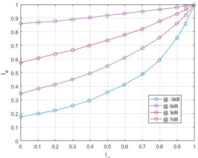
Moreover, by computing it by simulation, it allows us to take into account the effect of other components such as the equalizer for instance. An example of EXIT curve is given for a binary CPM with a RC pulse shape, a memory of L = 2 and h = 1/4 in Fig.1.11.

It has been shown that the area under the EXIT curve of an iterative component corre-sponds to its maximal achievable rate over the Binary Erasure Channel in [AKB04]. This

(45)

Figure 1.11 – EXIT charts for a binary CPM with a RC pulse shape, a memory of L = 2 and

h = 1/4

area is also considered as a good approximation for others channels and detectors [Hag04]; [LSL06]. Hence, this can be also used to estimate a lower bound of the maximum achievable rate Rú _{for the inner code and for a given signal to noise ratio. This lower bound is given by:}

Rú_Æ

⁄ 1 0

T (x)dx (1.40)

Readers unfamiliar with EXIT charts may refer to the tutorial by [Hag04].

EXIT charts analysis can be also used to compute by simulation the Spectral Efficiency (SE) of a CPM scheme. Indeed, the SE correspond to the achievable Information Rate (IR, noted I) for a given bandwidth. 1Hz is usually taken.

We can evaluate the SE by using:

„

SE = log2(M) ◊ Rú

BﬂT

(1.41) where T is taken equal to 1 and Bﬂis the considered bandwidth. We need a suitable definition

of the bandwidth. In fact, the Power Spectral Density (PSD) of CPM signals has an infinite support. However, almost all of the power is located only in a small portion. The most common definition is based on this power concentration, which assumes that the CPM signal bandwidth is the spectrum area that contains a given fraction ﬂ of the total power (usually