MASTER THESIS PRESENTED TO ÉCOLE DE TECHNOLOGIE SUPÉRIEURE
IN PARTIAL FULFILLMENT OF THE REQUIREMENTS FOR
THE MASTER’S DEGREE WITH THESIS IN MECHANICAL ENGINEERING M. A. Sc.
BY
Golnaz KHOSRAVI
PREDICTION OF BIOPARTICLES DISPERSION AND DISTRIBUTION IN A HOSPITAL ISOLATION ROOM
MONTREAL, 9th FEBRUARY-2016 © Copyright Golnaz Khosravi, 2016 All rights reserve
BY THE FOLLOWING BOARD OF EXAMINERS
Mr. Stéphane Hallé, Thesis Supervisor
Department of Mechanical Engineering at École de technologie supérieure
Mr. François Morency, Thesis Co-supervisor
Department of Mechanical Engineering at École de technologie supérieure
Pierre Bélanger, Chair, Board of Examiners
Department of Mechanical Engineering at École de technologie supérieure
François Garnier, Member of the jury
Department of Mechanical Engineering at École de technologie supérieure
THIS THESIS WAS PRESENTED AND DEFENDED
IN THE PRESENCE OF A BOARD OF EXAMINERS AND THE PUBLIC 2nd FEBRUARY-2016
“You are not a drop in the ocean. You are the entire ocean, in a drop.”
ACKNOWLEDGMENTS
Many people have contributed to the production of this thesis. I owe my gratitude to all those people who have made this dissertation possible and because of whom my graduate experience has been one that I will cherish forever.
My deepest gratitude is to my advisor Dr. Stéphane Hallé and my co-advisor Dr. François Morency. I have been fortunate to have advisors who gave me the freedom to explore on my own and at the same time the guidance to be on the right path. I am grateful for their patience, guidance, inspiration and continuous support throughout my master studies.
I would like to express my gratitude to my husband Ali and my brother-in-law Amir for his help and support. Special thanks to Maryam Ahmadi Golestan and Mehdi Kazeminia for their support at various stages of this research project. Last but not least, I am eternally grateful to my parents for their continuous encouragement and support throughout my life.
DEDICATION
PRÉVISION DE BIOPARTICULES DISPERSION ET DISTRIBUTION DANS DANS UNE CHAMBRE D'ISOLEMENT D'HÔPITAL
Golnaz KHOSRAVI RÉSUMÉ
L’extraction des bioaérosols dans une chambre d'isolement d’hôpital est importante pour réduire le risque de transmission de maladies infectieuses. La technique la plus courante pour protéger le patient, le médecin et les infirmières contre l’inhalation d’agents pathogènes est la ventilation. Le but de cette étude est de sélectionner, parmi plusieurs scénarios définis, le scénario de ventilation le plus efficace pour la chambre d'isolement étudiée. Pour atteindre cet objectif, l'influence du nombre de changement d'air par heure (ACH), l'angle d'injection (Ɵ) et la position de la grille d’extraction sur la concentration de bioaérosols expiré par un patient lors d’une toux, a été étudiée. La simulation numérique des écoulements (CFD) a été utilisée pour prédire l’écoulement d’air dans la chambre d’isolement et la concentration de bioaérosols. Une approche Euler-Lagrange a été utilisée pour étudier la dispersion des particules aéroportées et leurs dépôts dans la chambre modélisée. Le modèle mathématique pour l'écoulement d'air est basé sur les équations de Navier-Stokes moyennées (RANS) couplées au modèle de turbulence k-ɛ.
Un code CFD appelé Saturne a été choisi. Les résultats numériques obtenus du Code-Saturne ont été comparés à des résultats publiés dans la littérature. Pour étudier la capacité du Code-Saturne à prédire le dépôt de particules, des particules d'un diamètre de 1 µm à 10 µm, ont été injectés dans un canal. La vitesse de dépôt obtenue du Code-Saturne a été comparée à des résultats empiriques. Les résultats ont montré que le Code-Saturne a la capacité de prédire adéquatement la dispersion des particules dans un écoulement turbulent. Pour déterminer le système de ventilation le plus efficace, l'efficacité d'élimination des particules (PRE) et la concentration des particules dans la zone d’inhalation ont été comparés pour tous les scénarios simulés. Parmi les six scénarios de ventilation, celui avec un ACH = 15 et un angle d’injection de 45° a été choisi comme étant le scénario de ventilation le plus efficace.
Finalement, l’influence du positionnement de la grille d’extraction a été étudiée. Trois scénarios ont été considérés. Un scénario avec une extraction murale au-dessus de la zone d’occupation, un scénario avec une extraction murale près du plancher et un scénario avec une grille au plafond. Les simulations ont montré que le positionnement de la grille d’extraction a une influence importante sur l’élimination des contaminants et que l’extraction par le plafond présente la meilleure efficacité d'élimination des particules.
PREDICTION OF BIOPARTICLES DISPERSION AND DISTRIBUTION IN A HOSPITAL ISOLATION ROOM
Golnaz KHOSRAVI ABSTRACT
Removal of bioparticles from hospital isolation room is important in reducing the transmission risk of infectious diseases. An effective ventilation system is necessary to protect the patient, doctor and nurses from catching infectious diseases. The goal of this study was to select the most effective ventilation scenario for the investigated isolation room among the defined scenarios. To select the most effective ventilation scenario, the effect of air exchange rate (ACH), injection angle (Ɵ) and exhaust position on removing the exhaled bioparticles from a patient mouth during coughing process, was investigated. Computational Fluid Dynamic (CFD) was used for predicting the air flow pattern and bioparticle transmission. Bioparticle dispersion and deposition was modelled by an Eulerian-Lagrangian approach. The mathematical model for air flow was the Reynold Averaged Navier Stokes (RANS) equations with k-ɛ turbulence model. Code-Saturne was chosen as the CFD program and validated by numerical results and empirical equations. The numerical results obtained by Saturne were compared to results publish in the literature. To investigate the Code-Saturne capability to predict particle deposition, particles with different diameter in the range of 1 µm to 10 µm, were injected in a channel. Non dimensional deposition velocity obtained using Code-Saturne was compared to the empirical results available in the literature. The results showed that Code-Saturne has the capability of predicting the air flow pattern, particle dispersion and particle deposition.
For analyzing the results and choosing the most effective ventilation system, particle removal efficiency (PRE) and normalized particle concentration in the inhalation zone were compared. Among the six ventilation scenarios with different ACH and Ɵ, scenario with ACH=15 and Ɵ=45° was selected as the most effective. Finally, effect of exhaust position was investigated. Three scenarios were defined. The first one with an exhaust mounted on a wall near the ceiling, the second one with an exhaust mounted on a wall near the floor and the last one with an exhaust mounted on the ceiling. It is observed that the exhaust position has great influence on the air flow pattern and particle removal. It is found that an exhaust mounted on the ceiling scenario has the best particle removal efficiency.
TABLE OF CONTENTS
Page
INTRODUCTION ...1
CHAPTER 1 REVIEW OF LITERATURE ...7
1.1 Transmission of bioaerosols in indoor environment and their risk for health ...7
1.2 Determine an appropriate model for a cough process ...9
1.3 Ventilation strategies ...10
1.4 Role of ventilation systems ...11
1.5 Ventilation strategies used for improving indoor air quality ...11
1.6 Guidelines and standards ...13
1.7 Particular problem in the hospital sector and strategies for ventilation improvement ...13
1.8 Modeling the quality of indoor air ...15
CHAPTER 2 MATHEMATICAL MODEL AND METHODOLOGY ...19
2.1 Problem definition ...19
2.1.1 Coughing process problem ...19
2.1.2 Geometry and mesh ...20
2.1.3 Design of experiment ...25
2.1.4 Ventilation Scenarios ...26
2.1.5 Boundary conditions ...27
2.2 Procedures for predicting the particle dynamic behavior ...29
2.2.1 Code-Saturne Software ...29 2.2.2 Mathematical model ...29 2.2.3 Particle deposition ...36 2.2.4 Numerical method ...37 2.2.5 Code-Saturne validation ...38 2.3 Metrics selection ...40
2.3.1 Ventilation effectiveness ...41
CHAPTER 3 CODE-SATURNE VALIDATION ...43
3.1 Code-Saturne validation for prediction of air flow pattern and particle dispersion ...43
3.1.1 Chen et al [1] chamber geometry and mesh ...43
3.1.2 Boundary conditions ...45
3.1.3 Air flow pattern ...46
3.1.4 Particle dispersion ...47
3.2 Validation of Code-Saturne prediction of particle deposition ...53
3.2.1 Channel geometry and mesh ...53
3.2.2 Boundary condition ...54
3.2.3 Particle deposition ...54
CHAPTER 4 RESULTS AND DISCUSSION ...57
4.1 Results with different number of nodes ...57
4.2 Experimental design results ...58
4.3 Air flow pattern in the ventilated hospital isolation room ...60
4.4 Bioparticle distribution ...65
4.5 Ventilation effectiveness ...75
4.6 Ventilation strategies with different exhaust locations ...87
4.6.1 Ventilation strategy with an exhaust on the right wall ...88
4.6.2 Ventilation strategy with an exhaust near the floor ...89
4.6.3 Ventilation strategy with an exhaust on the ceiling ...89
4.6.4 Comparison of ventilation efficiency for three ventilation strategies with different exhaust positions ...90
CONCLUSION ...97
LIST OF TABLES
Page
Table 2-1 Selected Factors and levels for experimental design ...26
Table 2-2 Factor setting for experimental design ...26
Table 2-3 Selected ventilation scenarios with different levels of ACH and θ ...27
Table 2-4 Selected ventilation scenarios with different outlet positions ...27
Table 2-5 Air flow velocity at inlet 1 for each ACH ...28
Table 3-1 Calculated amount of non-dimensional particle relaxation time τ for each particle diameter. ...55
Table 4-1 PRE values for different types of mesh ...58
Table 4-2 PRE results for four preliminary scenarios ...59
Table 4-3 Comparison of pollutant removal efficiency for different ventilation scenarios ...76
Table 4-4 Comparison of pollutant removal efficiency for different ventilation strategies ...91
LIST OF FIGURES
Page Figure 2-1 Hospital isolation room geometry with an exhaust mounted on the
top of the left wall --- 21
Figure 2-2 Hospital isolation room geometry with an exhaust mounted on the bottom of the front wall --- 22
Figure 2-3 Hospital isolation room geometry with an exhaust mounted on the ceiling --- 23
Figure 2-4 Hospital isolation room mesh with 120000 cells --- 24
Figure 2-5 Energy consumption vs. Air change per hour (ACH) [84] --- 42
Figure 3-1 The geometry of the Chen et al. [1] chamber --- 44
Figure 3-2 A schematic of the meshed chamber --- 45
Figure 3-3 Comparison of Code-Saturne predicted and Chen et al. [1] x direction velocities at three different locations; a) x=0.2 m; b) 0.4 m and c) 0.6m --- 46
Figure 3-4 Comparison of Code-Saturne predicted and Chen et al. [1] particle concentration at three different locations a) x=0.2 m, b) 0.4 m and c) 0.6m --- 48
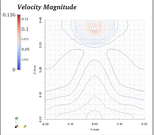
Figure 3-5 Velocity contours in plane F, located in the middle of the room in x direction --- 50
Figure 3-6 Particle concentration contours in a plane located in the middle of the room in x direction --- 51
Figure 3-7 Air velocity vectors in the plane F, located in the middle of the room in x direction. a) From the front view b) From right view c) From left view --- 52
Figure 3-9 A schematic view of the channel mesh --- 54 Figure 3-10 Comparison of CFD results and wood equation [78] --- 56
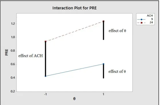
Figure 4-1 The value of PRE vs θ for two different levels of ACH --- 59 Figure 4-2 Effect of the parameters and their interaction effect on the PRE
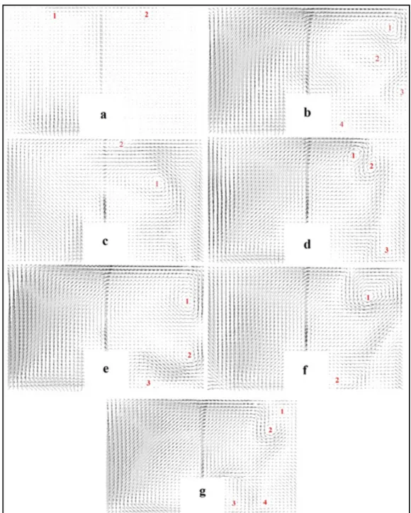
value --- 60 Figure 4-3 Airflow pattern, for ACH=24, Ɵ=45ᵒ, at t=10s of ventilation --- 61 Figure 4-4 Airflow pattern, for ACH=24, Ɵ=45ᵒ, at t=600s of ventilation --- 63 Figure 4-5 Air flow velocity vectors at plane C, for ACH=24 and Ɵ=45ᵒ, (a)
t=10s (b) t=100s (c) t=200s (d) t=300s (e) t=400s (f) t=500s (g)
t=600s of ventilation --- 64 Figure 4-6 Comparison of airflow pattern in plane B, for a) ACH=24, Ɵ=30ᵒ
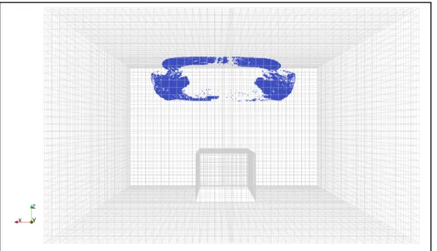
and b) ACH=24, Ɵ=45ᵒ, prior patient coughing --- 65 Figure 4-7 Bioparticle distribution after 1s injection ACH=24, Ɵ=45ᵒ --- 66 Figure 4-8 Bioparticle distribution in the 3D room with ACH=24, Ɵ=45ᵒ a few
seconds of ventilation --- 67
Figure 4-9 Bioparticle distribution in the 3D room with ACH=24, Ɵ=45ᵒ after a few 100s ventilation --- 67
Figure 4-10 Bioparticle distribution in the 3D room with ACH=24, Ɵ=45ᵒ after 400s ventilation --- 68 Figure 4-11 Bioparticle distribution the 3D room with ACH=24, Ɵ=45ᵒ after
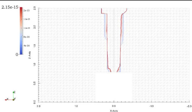
600s ventilation --- 68 Figure 4-12 Contours of particle concentration in the plane C for ACH=45,
Ɵ=45ᵒ after 1s of injection --- 69 Figure 4-13 Contours of particle concentration in plane C for ACH=24, Ɵ=45ᵒ
Figure 4-14 Contours of particle concentration in plane C for ACH=24, Ɵ=45ᵒ,
after 100s of ventilation --- 71 Figure 4-15 Contours of particle concentration in plane C for ACH=24, Ɵ=45ᵒ,
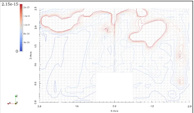
after 200s of ventilation --- 71 Figure 4-16 Contours of particle concentration in the plane C for ACH=24,
Ɵ=45ᵒ after 400s of ventilation --- 72 Figure 4-17 Contours of particle concentration in the plane C for ACH=24,
Ɵ=45ᵒ after 600s of ventilation --- 72 Figure 4-18 Contours of particle concentration in plane A for ACH=24, Ɵ=45ᵒ
after 1s of injection --- 73 Figure 4-19 Contours of particle concentration in the plane A for ACH=45,
Ɵ=45ᵒ after 100s of ventilation --- 74 Figure 4-20 Contours of particle concentration in plane A for ACH=24, Ɵ=45ᵒ
after 200s of ventilation --- 74 Figure 4-21 Contours of particle concentration in plane A for ACH=24, Ɵ=45ᵒ
after 600s of ventilation --- 75
Figure 4-22 Change of time efficiency for contaminants removal with ACH [53] --- 77 Figure 4-23 Air flow velocity over line D, above the patient mouth for six
different scenarios at time = 600s --- 78 Figure 4-24 Particle normalized concentration over line D, above the patient
mouth for six different scenarios after 600s ventilation --- 81 Figure 4-25 Particle normalized concentration over line E, where a doctor may
stand, for scenarios with Ɵ=30°, after 600s ventilation --- 82 Figure 4-26 Particle normalized concentration over line E, where a doctor may
stand, for scenarios with Ɵ=45°, after 600s ventilation --- 83 Figure 4-27 Velocity vectors in plane G, with y normal located at y= -2 m
(doctor position), for scenario with ACH=9 and Ɵ=30°, after 600s
Figure 4-28 Velocity vectors in plane G with y normal located at y= -2 m (doctor position), for scenario with ACH=24 and Ɵ=30°, after 600s
of ventilation --- 85 Figure 4-29 Velocity vectors in plane G with y normal located at y= -2 m
(doctor position), for scenario with ACH=15 and Ɵ=45°, after 600s
of ventilation --- 85 Figure 4-30 Percentage of deposited, removed and remained particles in room
after 600s ventilation for different ventilation scenarios --- 87 Figure 4-31 Airflow pattern, for ACH=15, Ɵ=45ᵒ, at t=10s of ventilation, for the
ventilation strategy with an exhaust mounted on the right wall --- 88 Figure 4-32 Airflow pattern, for ACH=15, Ɵ=45ᵒ, at t=10s of ventilation, for the
ventilation strategy with an exhaust near the floor --- 89 Figure 4-33 Airflow pattern, for ACH=15, Ɵ=45ᵒ, at t=10s of ventilation, for the
ventilation strategy with an exhaust located on the ceiling --- 90 Figure 4-34 Particle normalized concentration over line D, above the patient
mouth for three different scenarios after 600s of ventilation --- 93 Figure 4-35 Particle normalized concentration over line E, where a doctor may
stand, for three different scenarios, after 600s ventilation --- 95 Figure 4-36 Percentage of deposited, removed and remained particles in room
LIST OF ABBREVIATIONS
C Cunningham correction factor which account for the effect of slip C Mean particle concentration in a cell
C Time-averaged concentration of pollutants in the outlet
C Time-averaged concentration of pollutants in the breathing zone
D Particle mass diffusivity m2.s-1
d Particle diameter
m
dt Particle residence time s
F Drag force per unit particle mas kg.s-2
F Other forces exerted on the particle per unit mass N
F Saffman’s force N
g Gravitational acceleration vector m.s-2
g Non-dimensional gravity
K Boltzmann constant J.K-1
μ Fluid viscosity kg.m-1s-1
M Number flow rate of each trajectory N Number of particles p Pressure Pa ρ Density kg.m-3 ρ Particle density kg.m-3 ρ Air density kg.m-3 S Schmidt number
τ Wall shear stress Kg.m-1s-2
ϑ Kinematic viscosity m2.s-1
u Fluid velocity in x direction m.s-1
u Fluid velocity vector with component of (u, v, w) u Velocity vector of the particle
u Non-dimensional deposition velocity
u* Shear velocity of the fluid m.s-1
v Fluid velocity in y direction m.s-1
V Room volume m3
V Volume of a computational cell for particles m3
V Particle volume m3
w Fluid velocity in z direction m.s-1
INTRODUCTION
It is estimated that most people in urbanized countries spend more than 90% of their time in indoor environment [1]. So, the number of scientific studies about indoor air quality (IAQ) and its effects upon health has increased significantly in the past 10 years. U.S Environmental Protection Agency (EPA) ranks the indoor air pollution as the 5th environmental risks to public health in the US [1, 2, 3, 4]. The indoor air quality is represented by the pollutant concentrations in enclosed spaces. Indoor air quality affects the healthiness, the comfort, and the well-being of the occupants [5, 6]. Indoor pollutant such as dust, smoke, fungi and mists can penetrate into the respiratory system and cause negative health effects [1].
Indoor air quality problem exist in hospital sector just like in the other indoor places. However, in hospitals there is an elevated risk of infection with airborne infectious diseases from contagious patients [7, 8]. For example in a hospital outbreak in Canada, a super-spread of severe acute respiratory syndrome (SARS) epidemic happened due to airborne transmission [9]. In a hospital, some of the most important pathogen sources are: a potentially infectious patient, the personnel or the visitors and some hospital equipment like nebulizers [10].
More specifically, a patient in hospital isolation room can generate a significant amount of transmissible bioparticles such as mycobacteria, bacteria, viruses or fungi during a coughing process which includes a single cough event follows by breathing process. If the isolation room is not properly ventilated, airborne infectious diseases could spread easily and contaminate the personnel, the visitors or the other patients [11]. An airborne infection isolation room (AIIR) protects hospital workers, visitors and the other patients from exposure to infectious airborne transmitted from an infected patient [12, 13]. Airborne viruses, bacteria or microbes can be removed from isolation rooms by a highly effective ventilation system and a negative pressure differential with respect to the adjacent rooms. An appropriate
ventilation system in such rooms is one of the most important issue for engineers, which if fails can increase the pathogens spread within the hospital and thus contaminate more people and lead to hospital acquired infections [8, 14, 15].
According to ASHRAE Standard 170-2008, the recommended level of ventilation in a hospital isolation room is 10 air changes per hour (ACH) with two changes per hour of outdoor air (OA) [8]. These recommendations on the ACH should be respected to achieve a good air quality. To improve the air quality in an isolation room, the parameters which have influence on the ventilation effectiveness should be considered. Ventilation effectiveness and airborne dispersion strongly depends on some parameters such as the ventilation flow rates [17], the air distribution pattern [14, 18, 19], the position of air supplies (inlet) and exhausts (outlet) and the mechanism of atomization of airborne particles through breathing, coughing or sneezing [7, 10, 17 and 20]. An effective ventilation strategy is the one with particle removal efficiency (PRE) of at least 1 for enclosed spaces.
In order to improve the ventilation effectiveness, a good understanding of the fluid dynamic behavior of indoor air is needed. Ventilation measurements in full scale rooms can be expensive and may represent a health risk. Computational fluid dynamic (CFD) is an appropriate alternative which helps to study indoor air flow characteristics by solving conservation equations and predict airborne contaminant concentration and deposition for different ventilation scenarios.
The main objective of this project is to investigate the most effective ventilation scenario among a limited number of scenarios for removing the bioparticles exhaled by a patient mouth during a coughing process in a hospital isolation room. The scenarios were defined by changing three parameters; the air flow rate, the angle of incoming air and the exhaust position.
More specifically, it will:
• Introduce the previous works that studied the ventilation systems as a solution for decreasing bioparticle health risk to help us in reproducing some typical ventilation scenarios to remove the bioparticles effectively;
• Choose appropriate geometrical and mathematical model together with a numerical method for simulating airflow and bioparticle dynamic behavior into a 3 dimensional (3D) room during a cough process and propose different ventilation scenarios for investigations;
• Validate the 3D numerical simulation tools by comparing the air flow velocity, particle concentration and particle deposition velocity to available results in literature;
• Inject bioparticles into a 3D isolation room and investigate the air flow pattern and bioparticle dispersion for different ventilation scenarios;
• Compare the PRE values and particle concentrations to suggest the most effective ventilation scenario in diluting bioparticles for the room under investigation.
To choose the most effective ventilation strategy, the PRE values should be close to 1 or larger, the concentration of bioparticle in the inhalation zone should be as small as possible and the deposition of airborne particle should be limited.
To predict the dynamic behavior of a two-phase flow (fluid containing particles), an Eulerian-Lagrangian approach is used in which the particle phase is treated as a discrete phase and the fluid phase is considered as a continuum. In this work, the fluid phase is
modeled by the Reynolds Averaged Navier-Stokes (RANS) equations and the particle dispersion is modeled solving the momentum equation based on Newton’s law. In the Lagrangian frame, the equation of motion, resulting from the different forces exerted on the particle, is solved for each particle to compute their individual trajectory [21]. In this Master’s thesis, the airflow and particle dispersion models are predicted using an open source finite-volume based program, i.e., CFD package Code-Saturne (version 4.0.0) [22].
This memoir is structured as follows: Chapter 1 is devoted to the literature review, which presents the previous scientific articles available in scientific journals, relevant to bioparticle dispersion and effective ventilation systems. This chapter discusses the results of these previous works and their methodology to select the best method to find the most effective ventilation system for the investigated isolation room. Selected works to review are the researches focused on bioparticle transmission indoors and their risk for health. Also the literatures related to the cough process modeling are presented in this chapter. The other reviewed literatures focused on different ventilation strategies and the role of ventilation systems in improving the indoor air quality. The investigations that focused on the effective parameters on ventilation improvement in indoors particularly in hospital sectors were reviewed as well as the researches focused on the simulation of particle transport and distribution using CFD.
Chapter 2 defines the mathematical model and the methodology used to achieve our goals. This chapter begins with the problem definition. Then, an appropriate procedure for predicting the particle dynamic behavior is suggested. Finally, it introduces the useful metrics for evaluating the ventilation effectiveness.
Chapter 3 investigates the validity of Code-Saturne in predicting the airflow pattern and particle transport and deposition. First, it presents some comparison of the numerical results obtained by using the Eulerian-Lagrangian approach against the numerical results published in the literatures to validate the capability of Code-Saturne in prediction of air flow pattern
and particle dispersion. Then it compares obtained numerical results to some empirical results from literatures to validate the capability of the selected model in Code-Saturne to simulate accurately the particle deposition.
Chapter 4 presents the obtained numerical results and discusses them to find the most effective ventilation scenario in diluting the bioparticles for the defined hospital isolation room. It first presents the PRE results for meshes with different number of nodes to select a mesh that provides results accurately and efficiently. Then it represents the experimental design results and discusses the employed method for defining the scenarios with different air change rate (ACH) and angle of injected air (Ɵ) levels. The predicted air flow pattern and bioparticle distribution are also presented in this chapter. Thereafter, the results are compared to select the most effective ventilation scenario. For this purpose, the effects of two parameters: air change rate (ACH) and the angle of injected air in removing the bioaerosols from isolation room are studied and discussed. Finally, the effect of exhaust position is investigated and analyzed. The memoir ends with a general conclusion.
CHAPTER 1
REVIEW OF LITERATURE
The main objective of this chapter is to study and analyze the methods and outcomes of the relevant literatures about transmission of bioparticles. These literatures help us to define the problem and the geometrical model accurately and select an appropriate mathematical model and numerical method to find the most effective ventilation scenario for the defined isolation room. This chapter begins by a presentation of the transmission of bioaerosols in indoor environment and their risk for human health especially in the health care sector. Then an appropriate model for a cough process is determined. Thereafter, the ventilation strategies used by researchers for improving indoor air quality and the ventilation standards in hospitals are presented. Subsequently, results of seven investigations about indoors air dynamic behavior, in particular those that focus on improving the ventilation effectiveness in hospital isolation room, are presented. Finally, the methods used for modeling the quality of indoor air are mentioned.
1.1 Transmission of bioaerosols in indoor environment and their risk for health
Infection via inhalation of pathogens is termed airborne transmission. It occurs by spreading of either airborne droplet nuclei (typically 0.5 to 12 µm in diameter) or dust particles containing the infectious agents. Pathogens carried in this way can be widely dispersed by air flows and may become inhaled by a person close to the patient or may move a longer distance from the source patient. The distance that pathogens can move depends on factors such as their concentration, viability, diameter and aerodynamic behavior; as well as, environmental or physical conditions such as temperature, airflow and humidity [23]. Airborne transmission can cause nosocomial infections like tuberculosis, measles, chickenpox, severe acute respiratory syndrome (SARS) and flu (H1N1, bird flu, etc.). The cost related to the treatment of persons infected by airborne diseases represents a significant part of the health care system budget [24].
A large amount of droplets can enter the indoor air from a patient mouth by sneezing or coughing. First, these droplets are humid. After the release they start to dry-up and their diameter drop to 0.5-12 µm. Droplets with this new range of size are small enough to remain airborne and move passively through the air for a long period of time [9, 24]. According to Xie et al. (2007) [25] exhaled droplet nuclei are carried more than 6 m by sneezing while their initial velocity is around 50 m/s. Based on their results, coughing makes the droplet nuclei pass a distance more than 2 m while having an initial velocity equal to 10 m/s. Bolashikov et al. (2012) [8] reported that the initial peak of flow velocity generated by cough varies from 6 m/s up to 30 m/s.
The size and number of infectious airborne particle depend on the mechanism of generation, the age and the healthiness of the person who produced it. Different literatures present various amount for the size, number and the initial velocity of airborne particles. For example, Cole et al. (1998) [26] reported that coughing generates approximately 104 to 105 droplets. According to Marko Hyttinen et al. [33], sneezing generates up to 4×10⁴ droplets, while a cough or talking for 5 min produce 3×10³ droplet nuclei. Chao et al. (2009) [28] reported that the number of expelled droplets is 947 to 2085 per cough and 112 to 6720 during speaking.
Generally, the diameter of a virus is usually between 0.02-0.3 μm, a bacteria diameter is between 0.3-10 μm and fungal spore is 2-5 μm [24, 26]. Multiple pathogens are needed to create a sufficient level of infection for disease to be expressed. These pathogens need some larger aerosols like skin flakes, which are 13-17 μm in diameter or droplet with typical size of 20-40 μm in diameter, to be transported. About 95% of the respiratory generated droplets are smaller than 100 μm, while most of them are between 4-8 μm [27, 28, and 29]. Also, Yang et al. (2007) [30] reported that the coughing droplets size average is 8.35 μm. Papineni et al. (1997) [31], by means of improved diagnostics optical particle counting, showed that 80-90% of exhaled droplets in breathing or coughing are less than 1μm in diameter. Edwards
et al. 2004 [32] confirmed Papineni et al. [31] results by a similar experiment on 11 healthy human subjects. They suggested that inhaled particles during normal breathing are smaller than 1μm. Hyttinen et al. [33] in a review in 2011 reported that the size of coughed droplets is in the range of 0.6-16 μm and the average size is 8.4 μm. They mentioned that the size of droplet nuclei is between 0.6-5.4 μm, and 84% of them are smaller than 2.1 μm. Chao et al. (2009) [28] reported that the geometric mean diameter of the droplets exhaled during coughing is 13.5 μm and for speaking, it is around 16.0 μm.
1.2 Determine an appropriate model for a cough process
Considering the variety of the results about the size and number of exhaled particles during a cough, it is helpful to consider the studies that investigated the coughing droplet dynamic behavior in an isolation room. Zhang et al. [61] simulated a single cough in a 3D room. They injected 105 particles with a diameter of 1 µm from a patient mouth to investigate the particle dispersion by ventilation. Zhao et al. [35], injected particles with 1 µm diameter in two respiratory periods, with speed of 20 m/s to simulate two coughing process. Bolashikov et al. [8], simulated each cough by injecting CO2 for 0.8s with an initial velocity of 28.9 m/s. Kao [17], modeled a cough with duration of 1s and particle velocity of 8 m/s when ≤0.5s and particle velocity of 10 for 0.5 < ≤ 1 . Balocco [20] simulated a cough by injecting particles with velocity of 28 m/s for 1s and then modeled the breathing with an injection of air flow with a velocity of 0.9 m/s. Also, Alani et al. [34] simulated a cough with an injection of 2700 particles in a 3D room and investigated particles dispersion after 5 min ventilation. Although there is a variety of assumption for simulating a cough, the particle size and cough duration are similar in these literatures.
Based on the studies that simulated a cough process and investigated exhaled particle dispersion in a 3D room, a cough process including a single cough followed by breathing process could be modeled by injection of 105 bioparticles with diameter of 1 µm and a
velocity of 10 m/s for 1s injection duration and subsequently injection of air flow with a velocity of 0.9 m/s for breathing process [8, 34, 35].
1.3 Ventilation strategies
For diluting the bioparticles exhaled during a cough process, selection of an appropriate ventilation strategy is important. Different ventilation strategies make different air flow patterns, which have a significant influence on the pollutant removal efficiency in a room. There are two kinds of ventilation systems, mechanical and natural ventilation. Mechanical ventilation systems are the only appropriate systems for hospital sectors. In mechanical ventilation systems, fresh air is introduced to the building by using fan power. There are three different mechanical ventilation strategies: mixing ventilation, displacement ventilation and laminar flow ventilation [54, 57]. In mixing ventilation, the fresh air is introduced into the room by diffusers mounted on the ceiling or close to it. The air is blown at a relatively high speed and mixed with ambient air to have a homogeneous temperatures and homogeneous contaminant concentrations in the room. In displacement ventilation strategy, the air flow is transferred from the residence site close to the floor, up to the ceiling where it is evacuated through the exhausts. Air is introduced into the lower part of the space at a low speed and with a temperature lower than the room air. In this strategy, the air near the ceiling is warmer than the average air in the lower parts. Activities in the room create convective air flows from the floor to the ceiling. The displacement ventilation system is a good option for indoors ventilating and cooling together. However, this strategy has its drawbacks for heating [14, 55]. Laminar flow ventilation aims to create a flow with minimum turbulences where the air goes directly from the inlet to the extraction grid. This ventilation strategy is usually used in special cases like clean rooms [17, 56, and 57].
1.4 Role of ventilation systems
Room ventilation includes the admission of a mix of outdoor and treated recycle air into the enclosed space, the uniform distribution of this air and the extraction of contaminated air [36]. The main role of ventilation system is to remove pollutants such as bioaerosol and to provide healthiness, thermal comfort and well-being of occupants [37, 38]. In buildings, the ventilation must also remove specific pollutants such as carbon dioxide, formaldehyde and ozone. The origin of indoor aerosol may be respiratory activities, fuel burning, laser printers, food preparation and clean-up activities to name a few. Among indoor aerosol, biological particles can have adverse effect on human health, and many studies investigated bioparticles dispersion in ventilated indoors [39]. The dispersion of pollutants strongly depends on factors such as air change rates [8, 19], air distribution pattern [14], pressure difference with the surroundings [19], and the positioning of the ventilation diffusers to name a few [17, 18, and 40]. One way to improve indoor air quality is to simply increase air change rates to push the particles out more effectively. However it uses a considerable amount of energy, which is in conflict with building energy efficiency requirements [41]. Also according to Occupational Safety & Health Administration (OSHA) increasing the ACH from 25 to higher levels has no effect on indoor air quality [42]. So it is helpful to explore the effect of the air distribution pattern and the position of the ventilation diffusers such as inlet and outlet on indoor air quality with a constant source of contamination. Traditionally, mixing ventilation was the main method for the ventilation of indoor environment. Recently, displacement ventilation and personalized ventilation were commonly applied mainly for their low energy consumption and the better quality they provide [43].
1.5 Ventilation strategies used for improving indoor air quality
The first investigations of the indoor air quality date back to 1960’s decades. In those years, the main concern of researches was cigarette smoke, radon that is a radioactive gas that cause lung cancer and Sick Building Syndrome (SBS), or related building diseases [44, 45, and 46].
In recent years, the considerable increase of office equipment (computers, copiers, laser printers, etc.) and the widespread use of synthetic materials are among the causes responsible for the increasing problems of indoor air quality [47].
Yang et al. (2004) [48] studied the influence of ventilation strategies on the quality of indoor air in a chamber which is smaller than a real room. They have found that displacement ventilation creates a lower pollutant concentration level near the breathing zone than that by mixing ventilation. They concluded that with mixing ventilation, the contaminant is distributed more non-uniformly than with displacement ventilation. Therefore, they suggested that displacement ventilation performance is better for creating a healthy environment.
Bin Zhao et al. 2009 [49] indicated that, in the zone at height lower than 1 m, the ultrafine particles concentration in a room with a mixing ventilation mode is higher than that in a room with displacement ventilation, which is different for particles with micron size.
In another study by Jurelionis et al. (2015) [39], it is concluded that the location of the air diffusers and exhausts has a great effect on the quality of the ventilation process.
He et al. (2003) [50] published a study on the effects of contaminant source locations in a room ventilated by two ventilation strategies, displacement ventilation and mixing ventilation. They concluded that both systems are equally effective by measuring the normalized contaminant concentrations. Also, Cai et al. (2010) [51] found that the position of the contaminant source and the air extraction play an important role in the concentration of pollutants in indoor environment.
Qian et al. [14] investigated dispersion of exhaled droplet nuclei in a two-bed hospital ward with three different ventilation systems: mixing ventilation, downward ventilation and displacement ventilation. They concluded that displacement ventilation has been shown to provide better indoor air quality than the mixing ventilation in various environments such as offices. However, this conclusion is not applicable in hospital wards. They argued that the exhalation jet of a lying patient facing sideways can travel a very long distance along the exhaled direction assisted by the thermal stratification generated by the displacement ventilation. It could provide a high personal exposure level if the person is located in the exhalation jet area. So displacement ventilation is not suggested in hospital ward. From these investigations, it is concluded that although displacement ventilation strategy shows better performance in particles removal, it is not recommended for hospital sectors. Now it is important to have a look on the standards and guidelines for ventilation of hospital sectors.
1.6 Guidelines and standards
There are different guidelines and standards for the ventilation of health care facilities. Among them, the American Society of Heating, Refrigerating, and Air-Conditioning Engineers (ASHRAE) standard 170-2008 and Center of Diseased Control (CDC 2005) are the most usual ones [52, 53]. The ASHRAE 170 standard covers requirements to ensure adequate ventilation of healthcare facilities. This standard recommends at least 10 air changes per hour (ACH) for isolation rooms while this number according to CDC 2005 is 12 ACH.
1.7 Particular problem in the hospital sector and strategies for ventilation
improvement
Hospitals are the places where patients and other healthy people such as medical staff and visitors are in interaction every day. In hospital, people are in higher risk of being infected by
airborne infectious disease from patients [8]. Therefore, ventilation in healthcare facilities is an important issue since it provides protection from harmful emissions or airborne pathogenic materials to both patients and healthcare workers in addition to thermal comfort [58].
Kekkonen et al. (2014) [13], tested the performance of different ventilation scenarios in removal of airborne infection in isolation rooms by tracer gas techniques in which they concluded that locating air exhausts nearer to the patient result in more efficient contaminant reduction. To reach this conclusion, they compared the ratio between the gas concentration at the outlet grille and near the patient.
In 2006, Cheong and Phua [7] arrived at the same conclusion that nearer exhaust to the patient increases the particle removal by calculating another ratio called the pollutant removal efficiency index (PRE). Bolashikov et al. (2012) [8] investigated the effect of overhead mixing ventilation on amount of staffs and occupants exposure to coughed bioparticles in a hospital patient room with double-bed. They measured the concentration of the tracer gas and concluded that the level of exposure depended strongly on the doctor positioning and the distance from the infected patient and position of the coughing patient. Also, they declared, at a point within 1.1 m from the contaminant source, the maximum contaminant concentration at 12 ACH was much higher as compared to the maximum contaminant concentration at 6 ACH, which could be explain by the complex flow interaction around doctor’s body.
In 2011, Yau et al. [58] published a literature review about the ventilation of multiple-bed hospital in which they mentioned that a mechanical ventilation system significantly helps to improve the indoor air quality. They also concluded that mixing and displacement ventilations are the most prevalent strategies used for ventilation systems in hospital sectors.
Hyttinen et al. [33] in their literature review of experimental studies mentioned that for achieving a better protection of the healthcare workers, it is necessary to provide supply air from the ceiling in the front part of the room and make a direct air flow towards the patient. They declared that the results obtained about the location of exhaust air (outlet) whether it should be close to the patient head or ceiling level are not conclusive and need to be investigated more.
In 2010, Qian et al. [59] studied experimentally the distribution of expelled particles in an isolation room, with downward inlet and three different exhaust designs. They concluded that the ceiling-level exhausts are the most efficient strategy in removing expelled particles. Bin Zhao et al. [35] investigated the dispersion of droplets produced by the respiratory system. The results showed that droplets generated by normal breathing process move a relatively short distance, while droplets generated during coughing or sneezing can travel much longer distances, which increased the risk for workers and other patients to be affected by infectious patient.
From these investigations, it is concluded that the position of the diffusers are the most important factors that have effect on the ventilation effectiveness. Most of the researchers found that the exhaust position should be near the patient and on the ceiling to improve the ventilation effectiveness.
1.8 Modeling the quality of indoor air
There are two different methods to determine the airborne particles dispersion and distribution in indoors spaces. The first method is experimental studies, which provide information on particle transport and deposition in indoor spaces by specialized equipment such as Ultraviolet Aerodynamic Particle Sizer (UV-APS) and particle image velocimetry
(PIV). In this method, the potential danger for people during the measurements and the cost involved should be considered. In contrast, the second method, which is called computational fluid dynamics (CFD), provides a very cost-effective way to investigate the particle dynamic behavior in indoors environment [49, 60]. There are two approaches to model the two-phase flow problems and analyze the particle dispersion process with CFD. The first approach is the Eulerian-Eulerian model, in which the particle phase is considered as a continuum. The particle concentration is determined by solving the governing equations, which are derived from the mass conservation equation. The second approach is the Eulerian-Lagrangian model, in which the dynamic behavior of a single particle is determined by the trajectory method. In this approach, the air flow field is modeled by applying Reynolds averaged Navier-Stokes (RANS) turbulent models and the single-particle trajectory is modeled by solving the equation of motion. Various forces exerted on an individual particle drive the particle motion. With this model, it is necessary to analyze the dynamic behavior of a large number of sample particles to have statistically valid conclusions [61, 62].
The Eulerian-Eulerian approach involved Passive Scalar Model (PSM), Mixture Model (MIX) and Eulerian Model (EUL), while the Discrete Phase Model (DPM) belongs to the Eulerian-Lagrangian model. In PSM model, particles are considered as passive scalars, which means particles move in the same way as airflow and the inertia forces are ignored. The problem with this model is that only small particles could be assumed as passive scalar that do not have any interaction with the airflow. Discrete phase model (DPM) is a good alternative for PSM model, which is able to overcome the mentioned problem. In this model, all potential forces exerted on the particles are considered and the particle concentration could be determined from the individual particle trajectories [63]. DPM has been used in indoor airflow field prediction like in the Zhao et al. study in 2008 [21], Zhang et al. study in 2007 [61], Jiang et al. [63] work in 2012 and Alani et al [34] investigation in 2001. The major limitation of DPM is its need for much more computation time than Eulerian models. So considering this high computational cost, it is applicable for much diluted particle flows. In MIX and EUL models, both phases are treated as interpenetrating continuum and
interaction between the two phases are considered. Both of these models have been widely used in investigation of two-phase flow transportation [64, 65, and 66].
Choosing the Eulerian method or the Lagrangian method for simulating flows in a specific problem depends on the objectives and conditions of the problem. The most popular method for investigating particle concentration distribution in indoor spaces is the Eulerian method. For Lagrangian method, several researches declared that it can provide the detailed particle distribution, however it requires considerable computational efforts [61, 68, and 69]. In particular Zhang et al. [61] claimed that under steady state conditions, both Eulerian and Lagrangian methods were able to predict the particle concentration distributions in indoor environment. They concluded that the Lagrangian method is more capable in modeling particles transportation for unsteady diluted particle dispersion like modeling coughing state.
Zhao et al. [21] concluded that the Lagrangian model agrees well with the experimental data for the case studied, except at locations near the ceiling and inlet. They reported the largest relative error in particle concentration is 41.2% near the ceiling. They argued that the reason may be that the Lagrangian model assumes particles are trapped when reaching the walls. Jiang et al. [63] investigated particle dispersion and spatial distribution in a ventilated room using four different multiphase flow models, including PSM, DPM, MIX, and EUL. They concluded that only DPM could predict particle concentration distribution close to the experimental values. They argued that this model is the only one to take into account all the particle forces which are expected to affect the particle trajectories. Lai et al. [60], compared a new drift–flux Eulerian and a modified Lagrangian model for a single-zone chamber geometry. They concluded the two models agree very well for submicron particles.
In this study, we aimed to simulate the bioparticle dispersion and deposition, exhaled during a coughing process, in a ventilated isolation room to investigate the ventilation efficiency. In a coughing process the bioparticle concentration is low and we are in an unsteady air flow
condition. Zhang et al. [61] concluded that the Lagrangian method is more capable in predicting particles transmission for diluted particle dispersion in the unsteady condition. Thus, in this study the Lagrangian method was selected for the bioparticle dynamic behavior simulation.
CHAPTER 2
MATHEMATICAL MODEL AND METHODOLOGY
Now that the literature review has shown us that there is a need to improve ventilation system in isolation room to reduce the bioparticle hazard, a methodology to numerically investigate the ventilation systems will be propose in this chapter. The main objective is to propose geometrical and mathematical model plus a numerical method to simulate bioparticle dispersion and deposition after a cough into a ventilated isolation room. The first section of this chapter is dedicated to the problem definition. It begins with a description of the coughing process problem, the geometry and the mesh used for simulating coughing process. Then, the selected scenarios and the applied boundary conditions are described. In the next section, Code-Saturne software, the mathematical and numerical methods and the methods used for checking the validity and reliability of the code are presented. In the last section, the selected metrics for investigating the ventilation effectiveness are defined.
2.1 Problem definition
2.1.1 Coughing process problem
In this study, a coughing process includes a single cough event followed by the breathing process. Considering the literature review on the simulation of coughing processes, it was assumed that 105 particles were exhaled from the patient mouth in a single cough event [61]. According to the literature, the single cough event duration was assumed to be 1s [17, 20]. According to Xie et al. [25] the velocity of exhaled bioparticles in the coughing event was set to 10 m/s during 1s injection. For simulating the breathing process after the coughing event, the air velocity in the patient mouth was set 0.9 m/s [20, 25].
These bioparticles exhale from a patient mouth lying on a bed into an isolation room. The next section will define the geometry and the discretization of this isolation room.
2.1.2 Geometry and mesh
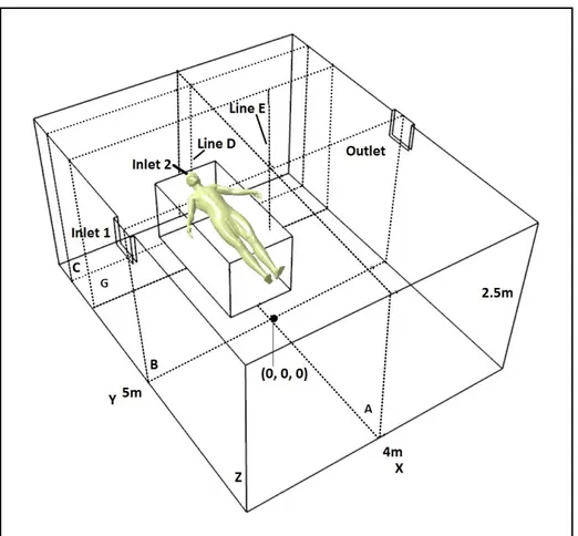
In this section the studied geometry is first defined. Then, the important zones of the studied hospital isolation room will be presented. The properties of the mesh and the procedure used to study the mesh effect on the results are described. The volume of the studied hospital isolation room was 50 m3 (4 m length × 5 m width × 2.5 m height), with the floor center located at (0, 0, 0) m and a patient lying on the bed as shown in Fig.2.1.
In the basic geometry, there are two inlets and one outlet. The fresh air is delivered to the room via a 0.4 m × 0.3 m rectangular diffuser located at the top of the left wall (inlet 1) and the contaminated air is extracted from the room via a 0.4 m × 0.3 m diffuser mounted on the top of the right wall (outlet). A bed of 1 m × 2 m × 0.8 m is located in the room. The bed and the patient are modeled as a rectangular box. The patient in the figure is only there for reader comprehension. The bioparticles were expelled from a square inlet (0.04 m × 0.04 m) used to model the patient mouth, which was located on the bed top surface with center at (0, -2.1, 0.8) m (inlet 2). To explore the particle concentration in patient breathing zone, line D, which was situated above the patient mouth, was defined at (0,-2.1, 0 ≤ z ≤ 2.5) m. The other important zone for investigating the particle concentration was the position of the doctor that was located at (-0.8, -2.0, 0 ≤ z ≤ 2.5) m. In addition, four planes were defined for studying the air flow pattern and particle concentration: plane A with center at (0, 0 and 1.25) m, plane B with center at (0, 0 and 1.25) m in the middle of room, plane C with center at (0, -2.1 and 1.25) m in the patient breathing zone and plane G with center at (0, -2 and 1.25) m in the doctor position.
The particle concentration is a dimensionless metric. It is defined as follows:
where is the number of particles, is the particle volume and is the room volume.
For investigating the effect of the exhaust position on ventilation efficiency, two other geometries were defined from the basic geometry. Fig. 2.2 shows the first modified geometry with an exhaust located on the front wall near the floor, with center at (-1, -2.5, 0.5) m. Fig. 2.3 shows the second modified geometry with an exhaust mounted on the ceiling with center at (-1.2, -1.65, 2.5) m. For these two geometries, the studied zone positions are the same as the ones in the first geometry in fig. 2.1.
Figure 2-1 Hospital isolation room geometry with an exhaust mounted on the top of the left wall
After defining the geometry, it is necessary to discretize the geometry and check that the results are not dependent on the constructed mesh.
Figure 2-2 Hospital isolation room geometry with an exhaust mounted on the bottom of the front wall
Fig. 2.4 shows the mesh used for the simulation of bioparticles dynamic behavior in the hospital isolation room. The number of grid point in a discretized geometry influences the solution accuracy and the required CPU time. Therefore, it is important to first check the effect of grid points on both computational accuracy and efficiency. As the number of grid points decreases, the computational time and the results accuracy decrease. So the selected mesh for the study is the coarser mesh that does not have a significant influence on the results accuracy. In building engineering, a difference less than 5% in PRE results is acceptable to conclude that the mesh does not influence the results accuracy [1, 63].
To investigate the effect of the mesh on the numerical results, three meshes with different number of cells were chosen. Only the basic geometry is used for the mesh study. The
Figure 2-3 Hospital isolation room geometry with an exhaust mounted on the ceiling
number of cells was chosen according to the previous similar works published in the literatures [10, 79].
• Dense mesh with 240 000 hexahedral cells;
• Moderately dense mesh with 120 000 hexahedral cells; • Coarse mesh with 60 000 hexahedral cells.
Figure 2-4 Hospital isolation room mesh with 120000 cells
The PRE was calculated for all of the above-mentioned meshes during the last 200s of a 600s simulation. In the last 200s, the results are stationary and do not change with time. The air flow was injected into the room from inlet 1 with a velocity of 2.77 m/s (ACH=24) and an injection angle of 45°. The Reynold number at inlet 1 is equal to 6.1×10⁴. In total, 105 bioparticles were injected into the room via inlet 2 (patient mouth) in one second with a velocity of 10 m/s. After one second, the injection is stopped and the air velocity is reduced to 0.9 m/s for simulating the breathing process.
Among these three meshes, the moderately dense mesh with 120 000 cells was selected for the study simulations. The differences between the PRE result of this mesh and the one of the dense mesh were 3.78 %. As mentioned before, in building engineering, a difference less than 5% is acceptable for concluding that the mesh does not affect the results [1, 63]. Also, the calculation time associated with the dense mesh was about 66 hours with a 2.5 GHz i7 processor, while the computation time for the same problem with the moderately dense mesh in the same computer equipment took “only” 24 hours.
In the selected mesh, the distance of the first grid node from the floor is equal to 0.016m. So the for the near wall cell is equal to 10.
2.1.3 Design of experiment
To define the parameter effectiveness’s on the results and choose a good range for the levels of these parameters, a two-level factorial design was used [80]. In this study, the effect of two parameters on PRE was investigated. The first parameter was the air flow rate (ACH) and the second one was the angle of the air flow injection at inlet (Ɵ). According to the literature, both of these parameters can change the air flow pattern in the hospital isolation room and thus the PRE [11, 19, 34, 59, 63, 76, and 79]. For each factor, the highest and lowest level were chosen. Table 2.1 shows the selected levels for each factor. Table 2.2 shows the factor setting for experimental design. For two factors with two levels, the total number of preliminary tests is equal to:
Table 2-1 Selected Factors and levels for experimental design
Factor Lowest level (-1) Highest level (+1)
θ 30° 45°
ACH 9 24
The levels of each parameter for four preliminary tests are shown in table 2.2. PRE values were calculated for each test. Effects of each parameter (and their levels) on the results were calculated. Knowing the effect of each parameter and levels helped us to choose the other levels and define the new scenarios for further investigation.
Table 2-2 Factor setting for experimental design
2.1.4 Ventilation Scenarios
According to the results obtained by experimental design, six scenarios were defined. Table 2.3 shows the selected ventilation scenarios.
No. θ ACH
1 +1 +1 2 -1 -1 3 +1 -1 4 -1 +1
Table 2-3 Selected ventilation scenarios with different levels of ACH and θ Scenarios θ ACH Scenario 1 45˚ 24 Scenario 2 45˚ 15 Scenario 3 45˚ 12 Scenario 4 45˚ 9 Scenario 5 30˚ 24 Scenario 6 30˚ 9
Also to investigate the effect of the outlet position on the ventilation efficiency, three new scenarios were defined in table 2.4.
Table 2-4 Selected ventilation scenarios with different outlet positions
Scenarios θ ACH Exhaust position
Scenario A 45˚ 15 On the right wall
Scenario B 45˚ 15 On the front wall near the floor
Scenario C 45˚ 15 On the ceiling
2.1.5 Boundary conditions
For hospital isolation room study, all variables were defined at the two inlets. The air was supplied to the room at inlet 1 in four different air change rates (9, 12, 15 and 24 ACH), and
in two different injection angles (30° and 45°). Table 2.5 shows the air flow velocity at inlet 1 for each ACH. For simulating the coughing process, 105 bioparticles with diameter of 1 µm and density of 1100 kg/m3 [31, 61], were injected into the room for one second, from the patient mouth, at inlet 2.
Table 2-5 Air flow velocity at inlet 1 for each ACH
ACH Air flow velocity (m/s)
24 2.77 15 1.73 12 1.38 9 1.04
The particle concentration was normalized by the concentration at inlet 2, therefore the particle concentration expelled by the patient was assumed to be 1. For the outlet, a Dirichlet boundary condition was set for pressure and a Neumann boundary condition was applied for velocity, i.e their normal derivative was equal to zero [1, 35]. Additionally, for solid walls, no-slip boundary condition was applied. The air was assumed to be isothermal and incompressible.
The Reynolds numbers were calculated based on the inlet hydraulic diameters and the air flow velocity. The Reynolds number at inlet 1 was in the range of 2.3 × 10⁴ to 6.1 × 10⁴, which means that the airflow was turbulent for all the applied ACHs namely 9, 12, 15 and 24. The Reynolds number at inlet 2 during particle injection was equal to 2.6 × 10⁴, which was also in the turbulent flow range.
2.2 Procedures for predicting the particle dynamic behavior
After problem definition, it is important to choose the appropriate mathematical model and numerical method for simulating the bioparticle dispersion and deposition in the ventilated isolation room.
2.2.1 Code-Saturne Software
Code-Saturne [22] is an open source computational fluid dynamics software which was developed in 1997 at Electricité de France (EDF) R&D. This software is based on a co-located Finite Volume approach that accepts meshes with different types of cell such as tetrahedral, hexahedral, prismatic, pyramidal, and polyhedral. Also, it accepts different types of grid structures such as unstructured, block structured, hybrid, conforming and with hanging nodes. Code-Saturne solves the Navier-Stokes equations for 2D, 2D-axisymmetric and 3D flows, steady or unsteady, laminar or turbulent, incompressible or weakly compressible, isothermal or not, with scalars transport if required. There are several turbulence models available in Code-Saturne such as Large Eddy Simulations, Reynolds-Averaged Navier-Stokes (RANS) models, like the k-ɛ model and Reynolds Stress model. Particle-tracking with Lagrangian modeling is available in this code as a specific module [69].
2.2.2 Mathematical model
2.2.2.1 Air flow simulation
The Navier-Stokes equations are the basic relations in the field of fluid dynamics that can predict Newtonian flow dynamic behavior. We present here the governing equations for the prediction of incompressible Newtonian laminar flow movement:
1- Continuity equation
= 0 (2.3)
2- Equation of motions (Navier-Stokes equations)
+ ( ) = + (2.4) + ( ) = + (2.5) + ( ) = + (2.6)
In above Equations, u, v and w are the fluid velocity in x, y and z direction, is the fluid velocity vector with component of (u, v, w), t is the time, is the kinematic viscosity, ρ is the density and p is the pressure.
To predict the turbulent flow motion, it is necessary to replace in the above equations the flow variables u, v, w and p, by the sum of a mean and fluctuating component. So by putting = + ´ , = + ´ , = + ´ and = + ´, the Navier-Stokes equations for turbulent incompressible flow is achieved, where U, V and W are the mean values of velocity,
P is the mean value of pressure, ´ , ´, ´ ´ represent the turbulent flow fluctuations. Then, the time average of these equations gives the RANS equations:
+ = − + + − − (2.7)
+ = − + + − − (2.8)
+ = − + + − − (2.9)
The averaging process results in new unknown terms, such as , , which are called the Reynolds stresses. The determination of the Reynolds stress terms requires extra equations that are solved with turbulence models [70, 71].
The most common turbulence models are: zero equation models like the mixing length model, two equations models like the k-ɛ model, the Reynolds stress equation model, the algebraic stress model and the large eddy simulation.
To simulate the airflow dynamic behavior, the k-ɛ model [69] was employed by using the scalable wall function for smooth walls. This turbulence model is a general description of turbulence in which two transport partial differential equations (PDE), one for the turbulent kinetic energy k, and the other one for the rate of dissipation of turbulent kinetic energy ɛ, are solved. Also, scalable wall functions overcome the problem associated with low y+ values of the near-wall grid. The y+ value of the grid points closest to the wall can no longer be in the log law region as presumed by wall functions. This occurs either with excessively fine grids or with moderately refined grids in the area close to the wall. [70, 72, 69].
2.2.2.2 Particle motion
Code-Saturne can predicts the trajectory of a discrete phase particle by integrating the force balance on the particle using the Lagrangian approach. This method solves the momentum equation in which the particle inertia is equated with the forces acting on the particle based on Newton’s law:
= − + + (2.10)
Where is the velocity vector of the particle; is the velocity vector of air; − is the drag force per unit particle mass which is the force exerted on the particle due to the velocity gradient between the fluid and the particle and acts in a direction opposing the flow; and are the particle and air density respectively; is the gravitational acceleration vector and represents the other forces per unit mass.
Since Re (based on particle diameter) is less than one for particles in the micrometer range, the drag force derived from the Stokes’s law in slip condition is as follows
= − = − (2.11)
where is the fluid kinematic viscosity; is the particle diameter and is the Cunningham correction factor which account for the effect of slip. Small particles with diameter equal or less than the mean free path of the gas, settle faster than predicted by Stokes’s law in continuum regime, due to the slip at the surface of the particle. So in slip condition, the drag force decreases compared to the one obtained by Stokes' law in
continuum regime. Thus, in slip condition, the Cunningham correction factor is used in order to correct this difference [73]:
= 1 + (1.257 + 0.4 .
) (2.12) where λ is the mean free path of the molecule which is equal to 66 nm at standard
temperature and pressure, and = 1.1 for particles with a diameter of 1 µm [73].
The second part of the right-hand side of Eq. 2.10, , is the gravitational force minus the buoyancy force on the particle per unit mass. The last term, represents other forces exerted on the particle which includes the Basset history term, the pressure gradient, the virtual mass force due to unsteady flow, the Brownian and Saffman’s lift force caused by shear and thermophoretic force due to temperature gradient. The effect of these forces depends on the particle properties and flow condition. For fine particles in enclosed spaces, the Basset history, the pressure gradient and the virtual mass force are negligible. Also, regarding the isothermal assumption for this study, the thermophoretic force is negligible [21, 63 and 62].
The effect of Brownian motion can be optionally included in other forces ( ) for sub-micron particles, especially for non-turbulent models. The lift force, which is called the Saffman’s force ( ) can also be included in other forces ( ) as an option for sub-micron particles. Lift force is only valid in an infinite domain and, therefore, should not be considered in the vicinity of a wall [83].
The equation of motion of the particles used for this study was based on the following assumptions:
1- The particles are rigid spheres.
2- The diameter of particles was 1µm and the simulation is in a ventilated room, thus the contribution of the Saffman’s lift force and Brownian force in the movement of particles was small and could be neglected [62].
3- Because of the low concentration of the particle, collision between particles is negligible.
4- It was assumed in this study that the presence of particles in the fluid does not affect the structure of the turbulent flow (one-way coupling assumption). The one-way coupling assumption means that the fluid affects the movement of particles, but the particles do not influence the movement of fluid. This assumption is reasonable when the mass concentration of the particles is much smaller than the density of air, which is the fact in coughing simulation.
So the trajectory equation used in this study is:
= − + (2.13)
The turbulent dispersion of the particles is modeled by a stochastic approach. In this approach, adopted by Code-Saturne, the trajectory equation for each particle was predicted by integrating the trajectory equation, using the instantaneous fluid velocity, + along the particle path. Here, the mean velocity of air flow, was obtained by solving the RANS equations using the k-ɛ turbulence model. The instantaneous velocity was modeled by stochastic PDF (Probability Density Function) approach solving Langevin equation,

![Figure 3-3 Comparison of Code-Saturne predicted and Chen et al. [1] x direction velocities at three different locations; a) x=0.2 m; b) 0.4 m and c) 0.6m](https://thumb-eu.123doks.com/thumbv2/123doknet/7702680.245888/70.918.111.727.454.947/figure-comparison-saturne-predicted-direction-velocities-different-locations.webp)