Universit´e de Montr´eal
Entity-centric representations in deep learning
par Rim Assouel
D´epartement d’informatique et de recherche op´erationnelle Facult´e des arts et des sciences
M´emoire pr´esent´e `a la Facult´e des arts et des sciences en vue de l’obtention du grade de Maˆıtre `es sciences (M.Sc.)
en informatique
Juin, 2020
c
Universit´e de Montr´eal Facult´e des arts et des sciences
Ce m´emoire intitul´e:
Entity-centric representations in deep learning
pr´esent´e par: Rim Assouel
a ´et´e ´evalu´e par un jury compos´e des personnes suivantes: Pierre-Luc Bacon, pr´esident-rapporteur
Yoshua Bengio, directeur de recherche Hugo Larochelle, membre du jury
Résumé
L’incroyable capacit´e des humains `a mod´eliser la complexit´e du monde physique est rendue possible par la d´ecomposition qu’ils en font en un ensemble d’entit´es et de r`egles simples. De nombreux travaux en sciences cognitives montre que la perception humaine et sa capacit´e `a raisonner est essentiellement centr´ee sur la notion d’objet. Motiv´es par cette observation, de r´ecents travaux se sont int´eress´es aux diff´erentes approches d’apprentissage de repr´esentations centr´ees sur des entit´es et comment ces repr´esentations peuvent ˆetre utilis´ees pour r´esoudre plus facilement des tˆaches sous-jacentes.
Dans la premi`ere contribution on montre comment une architecture centr´ee sur la notion d’entit´e va permettre d’extraire des entit´es visuelles interpretables et d’apprendre un mod`ele du monde plus robuste aux diff´erentes configurations d’objets.
Dans la deuxi`eme contribution on s’int´eresse `a un mod`ele de g´en´eration de graphes dont l’architecture est ´egalement centr´ee sur la notion d’entit´es et comment cette architecture rend plus facile l’apprentissage d’une g´en´eration conditionelle `a certaines propri´et´es du graphe. On s’int´eresse plus particuli`erement aux applications en d´ecouverte de m´edicaments. Dans cette tˆache, on souhaite optimiser certaines propri´et´es physico-chmiques du graphe d’une mol´ecule qui a ´et´e efficace in-vitro et dont on veut faire un m´edicament.
Mots-Cl´es: apprentissage profond, apprentissage non supervis´e, apprentissage de repr´esentations, repr´esentations d’objets, repr´esentations de graphes, d´ecouverte de m´edicaments
Summary
Humans’ incredible capacity to model the complexity of the physical world is possible because they cast this complexity as the composition of simpler entities and rules to process them. Extensive work in cognitive science indeed shows that human perception and reasoning ability is structured around objects. Motivated by this observation, a growing number of recent work focused on entity-centric approaches to learning representation and their potential to facilitate downstream tasks.
In the first contribution, we show how an entity-centric approach to learning a transition model allows us to extract meaningful visual entities and to learn transition rules that achieve better compositional generalization.
In the second contribution, we show how an entity-centric approach to generating graphs allows us to design a model for conditional graph generation that permits direct optimisation of the graph properties. We investigate the performance of our model in a prototype-based molecular graph generation task. In this task, called lead optimization in drug discovery, we wish to adjust a few physico-chemical properties of a molecule that has proven efficient in vitro in order to make a drug out of it.
Keywords: representation learning, unsupervised learning, deep learning, entity-centric representations, objects, graphs generation, graph neural networks, conditio-nal generation, drug discovery.
Table des matières
R´esum´e . . . iii
Summary . . . iv
Contents . . . v
List of Figures. . . vii
List of Tables . . . ix List of Abbreviations . . . x Acknowledgments . . . xi 1 Introduction . . . 1 1.1 Background . . . 1 1.1.1 Machine Learning . . . 1
1.1.2 Unsupervised vs Supervised Learning . . . 1
1.1.3 Representation Learning . . . 2
1.1.4 What is a good representation ? . . . 3
1.2 Motivation . . . 4
1.2.1 Objects and Representation Learning . . . 4
1.2.2 First Contribution : SPECTRA . . . 5
1.2.3 Graphs and Deep Learning . . . 5
1.2.4 Second Contribution : DEFactor . . . 6
1.3 Visual Entity-centric Representations . . . 7
1.3.1 Generative Modeling . . . 7
1.3.2 Variational Inference and Learning . . . 7
1.3.3 Slot-based Representations . . . 8
1.3.4 Scene-Mixture Models . . . 9
1.4 Molecular Graphs and Deep Learning . . . 12
1.4.1 Molecular Graph . . . 12
1.4.3 Molecular Graph Optimization. . . 13
2 SPECTRA : Sparse Entity-centric Transitions . . . 15
2.1 Abstract . . . 16 2.2 Introduction . . . 16 2.3 Related Work . . . 18 2.4 SPECTRA. . . 19 2.4.1 Model overview . . . 20 2.5 Experiments . . . 22
2.5.1 Learned Primitive Transformations . . . 22
2.5.2 Structured Representation Learning . . . 24
2.5.3 Intrinsic Exploration Strategy . . . 26
2.6 Conclusion and Future Work . . . 28
2.7 Architecture and Hyperparameters . . . 28
2.7.1 Fully observed setting . . . 28
2.7.2 Latent setting . . . 30
2.8 Additional Visualisations . . . 31
3 DEFACTOR : Differentiable Edge Factorization-based Probabi-listic Graph Generation . . . 35
3.1 Abstract . . . 36
3.2 Introduction . . . 36
3.3 Related work . . . 37
3.4 DEFactor . . . 39
3.4.1 Graph Construction Process. . . 39
3.4.2 Training . . . 42
3.4.3 Conditional Generation and Optimisation . . . 44
3.5 Experiments . . . 45
3.6 Future work . . . 49
3.7 Models Comparison . . . 49
3.8 Conditionnal setting . . . 50
3.8.1 Graphs continuous approximation . . . 50
3.8.2 Mutual information maximization . . . 51
3.8.3 Reconstruction as a function of number of atoms . . . 51
3.8.4 Visual similarity samples . . . 52
4 Conclusion . . . 54
Table des figures
2.1 A: SPECTRA. Illustration of an entity-centric transition model. B: Naive Perception module with a CNN-based encoder and a slot-wise decoder. . . 18
2.2 left: Full and sparse settings are trained on environment contai-ning one box and evaluated out-of-distribution on two boxes. We plotted the validation losses of both settings during training. The full connectivity architecture is unable to achieve out-of-distribution generalization to an environment with two boxes. right: Illustration of what the model has to learn in the fully observed setting: to be correct the model needs to map any concatenation of [agent,move] to a vacated position = floor and to select only the right entities to be changed. The learned mappings are general rules that are directly transferable to settings with more boxes. . . 23
2.3 Comparison of slot-wise masked decodings when the perception mo-dule is trained separately or jointly with the sparse transitions. We show the reconstruction associated with the slots that contain in-formation about the agent. When the perception module is trained jointly, slots in the learned latent set are biased to be entity-centric (here agent-centric). . . 24
2.4 Loss vs training updates, with training is done in pixel space, tran-sitions are sampled randomly and results are averaged over 3 runs. left: Validation perception loss Lpercep of joint and separate training
right: Validation transition loss Ltrans of joint and separate training.
Separate training is better in terms of perception loss but joint trai-ning gives a better transition model. We posit that this is because the slots are biased to be entity-centric and transformations involving only relevant entities are easier to learn. . . 25
2.5 Comparison is done against randomly sampled transitions. left: Num-ber of entities changed in the 1-step buffer during training. As expec-ted, the number of transitions with 2 spatial locations changed in the grid increases whereas the ones with no location changed decreases. We also notice a slight increase in the number of transitions with 3 spatial locations changed (corresponding to the agent moving a box !). Training is done in the fully observed setting. right: Training done in pixel space. Again here, the number of transitions with two spatial locations changed in the grid increases whereas the ones with no location changed decreases. However the number of of transitions with the agent that moves a box did not increase. . . 27
2.6 Transition model with and without selection phase. . . 30
2.7 Additional visualisations of masked decodings from joint and separate training settings. . . 32
2.8 Additional visualisations of masked decodings from joint and separate training settings. . . 33
2.9 Additional visualisations of masked decodings from joint and separate training settings. . . 34
3.1 Overview of our molecule autoencoding ((a) and (b)) and conditional generation (c) process. . . 38
3.2 Conditional generation: The initial LogP value of the query molecule is specified as IL and the Pearson correlation coefficient is specified as c. We report on the y-axis the conditional value given as input and on the x-axis the true LogP of the generated graph when translated back into molecule. For each molecule we sample uniformly around the observed LogP value and report the LogP values for the decoded graphs corresponding to valid molecules. . . 47
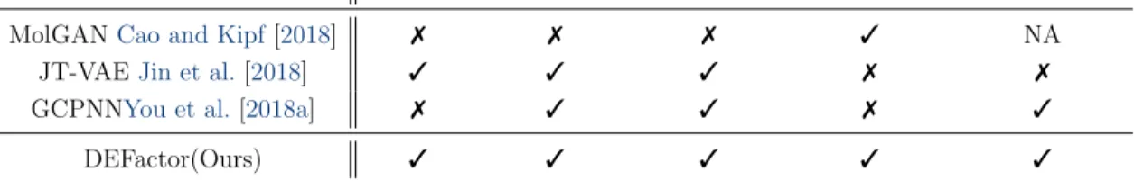
3.3 We report here a comparison of the abilities of previous recent models involving molecular graph generation and optimization . . . 49
3.4 Partial graph Autoencoder used for the pre-training part . . . 50
3.5 Accuracy score as a function of the number of heavy atoms in the molecule(x axis) for different size of the latent code . . . 52
3.6 LogP increasing task visual example. The original molecule is circled in red. . . 53
Liste des tableaux
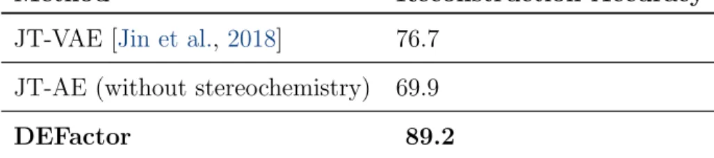
3.1 Molecular graph reconstruction task. We compare the performance of our decoder in the molecular reconstruction task with the JT-VAE. The results for JT-VAE result is taken from Jin et al. [2018].. The JT-AE refers to an adapted version of the original model using the same parameters. It is however deterministic, and like DEFactor does not evaluate stereochemistry.. . . 46
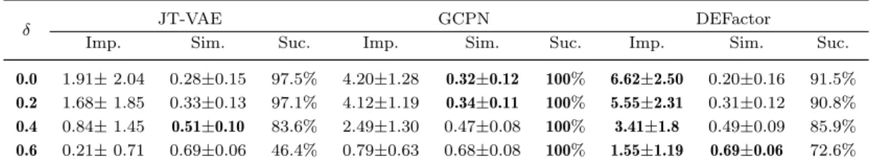
3.2 Constrained penalized LogP maximisation task: each row gives a different threshold similarity constraint δ and columns are for im-provements (Imp.), similarity to the original query (Sim.), and the success rate (Suc.). Values for other models are taken from You et al. [2018a]. . . 48
List of Abbreviations
ML Apprentissage Machine de l’anglais Machine LearningMLE Estimation du Maximum de Vraisemblance de l’anglais Maximum Likelihood Estimation
MI Information Mutuelle de l’anglais Mutual Information
MLP Perceptron Multicouche de langlais Multi Layer Perceptron
RL Apprentissage par renforcement de l’anglais Reinforcement Learning
DRL Apprentissage par renforcement profond de l’anglais Deep Reinforcement Learning
VAE Auto-encodeur variationnel de l’anglais Variational Autoencoder MSE Erreur quadratique moyenne, de l’anglais Mean Square Error
GAN Reseaux de Neuronnes adversariaux generatif de l’anglais Generative Adver-sarial Networks
GNN Reseaux de Neuronnes pour Graphs de l’anglais Graph Neural Networks GMM Mod`ele `a Mixture de Gaussiennes de l’anglais Gaussian Mixture Model
Acknowledgments
First and foremost, I would like to thank my supervisor Yoshua Bengio without whom I would not have considered joining this amazing research journey. Thank you for giving me the ideal amount of research freedom that allowed me to eventually find my own path and research interests. I am truly grateful to have such an inspiring and understanding person to guide me through this adventure. With you I made it through this first milestone and this is all just starting !
I would also like to thank all the amazing friends I made in Montreal who’ve been unconditionally supportive: Ahmed, Amal, Anne-Marie, Arthur, Vincent, Carla, Julie, Maxime, Salem, Gauthier, Adrien, Victor, Zhor, Nazia ... to name a few. Furthermore, I am very grateful for the many members of Mila, who I crossed paths with in my time pursuing a master’s. I just love the vibe of the lab and I truly found a new home abroad thanks to all of you. It all started with Salem agreeing (did he have the choice ?) to be my buddy and answer the hundred questions I had a day, Ahmed and that couscous party, Gauthier and his shared taste for chocolate, Adrien always free for a chill Friday afternoon at the lab, Tristan that I still call Yann junior, and re-inventing objects with Evan. Those tea talks also kept me pretty busy the whole time.
To Benjamin and Prof. Satoh, thank you for taking a chance on me and giving the opportunity to discover Tokyo, research and the field of machine learning as part of my NII experience. To Pierre, Simon, Gilles and all the amazing Owkin people I met back in Paris without whom I wouldn’t have even applied to Mila.
To Marwin, Mo and Amir, this amazing Benevolent.AI trio ! I know I was a stubborn collaborator from time to time but working with you on DEFactor was real fun. I not only learned a lot on drug discovery and graphs in general but it made me realize the importance of good and frequent communication in research.
Last but not least, a huge thank to my mom, Khadija, my brother, Amine, and my sister, Nour, for believing in me more than I do !
1
Introduction
1.1
Background
1.1.1
Machine Learning
The desire to understand human cognition has generated a variety of scientific disciplines. Cognitive science, neuroscience, and the study of machine learning and artificial intelligence (AI) are the most popular examples. The work in this thesis is situated in the field of machine learning, which is one of the most pursued branches in AI research. Machine learning deals with the question of buildingg systems and designing algorithms that learn from data and experience which is in contrast to the traditional approach in computer science where systems are explicitly programmed to follow a sequence of instructions.
More particularly in machine learning we seek to learn algorithms that are necessary to solve one or several tasks. In traditional computer science a programmer would specify the algorithm (the set of instructions) for the machine to satisfy the desired task whereas machine learning would shift this algorithm creation process to the computer based on some input data. Understanding this thesis will require basic knowledge of machine learning, and more specifically deep learning. For a full introduction to machine learning and deep learning, we encourage the reader to check outBishop [2006], Murphy [2012], Goodfellow et al. [2016]
1.1.2
Unsupervised vs Supervised Learning
Machine learning algorithms are traditionally divided into two main learning pa-radigms: supervised learning and unsupervised learning methods. Supervised learning usually involves learning from a dataset of inputs x and their associated label y provided by humans. The goal of supervised learning is then to learn a mapping f linking x to y. Most of the existing algorithms will do so by trying to
model the distribution p(y|x) with x, y ∼ (X, Y ) [Goodfellow et al.,2016].
On the hand, unsupervised learning designates learning paradigms that only make use of unlabeled input data x∼ X. The objective can vary from one task to another but it often involves estimating or sampling from the input distribution P(X). Unsupervised learning can also be used as an intermediary to learn a good representation of the data which is of particular interest in this thesis. Four common goals of unsupervised learning are [Khemakhem et al., 2019]:
— Density Estimation
Modelling the data distribution, pdata(x), is often concerned with fitting a
model pmodel(x) to estimate the data density.
— Sampling
Sampling involves learning a model that allows you to perform approximate sampling from pdata(x). This can be accomplished using density estimation if
you learn a model you can sample from. Moreover, one could directly learn a generator function made specifically for sampling [Goodfellow et al., 2014a]. — Underlying Structure of the Data
In this case, we are interested in revealing underlying structure of the data. We can often imagine the data is created by some unknown generative process that takes a few underlying high level concepts and combines them to form the raw data. In this case we are interested in discovering these hidden concepts that are part of this data generating process.
— Downstream Task performance
In this case, we aim to learn transformations of the data, which we call repre-sentations, that are amenable to future prediction tasks. This is commonly called representation learning.
These four goals are interrelated, and not mutually exclusive. In this thesis we will focus on a certain type of representations that should help the downstream task performance when the compositional aspect is of major importance.
1.1.3
Representation Learning
The problem of learning is commonly approached by fitting a model to data with the goal that this learned model will generalize to new data or experiences. Traditionally, many machine learning algorithms are built on top of some features,
extracted using a pre-defined procedure from the raw data format. The process of developing sophisticated feature extractors is often referred to as feature engineering. On the other hand deep learning (DL), addresses the learning problem by jointly learning representations of the raw input data and a predictive model for the task at hand. This is usually achieved by stacking multiple layers of differentiable non-linear transformations and by training such a model in an end-to-end fashion using gradient descent approaches.
Performance of machine learning algorithms is often dependent on the data representations they use for their input. A representation is traditionally [Goodfellow et al.,2016] defined as a transformation of the input data into another space, usually of a lower dimension before it is used by the machine learning algorithm. The field of representation learning designates all the methods used to learn these transformations from raw input data instead of having to specify a function to extract hand-crafted features [Lowe, 2004, Horn and Schunck, 1981]. As such representation learning has been defined as representing data in a way that will facilitate some downstream tasks [Bengio et al., 2013]. Recently, representation learning has become synonymous with unsupervised representation where we want to learn a representation useful for many tasks without knowing the task of interest beforehand.
1.1.4
What is a good representation ?
We want a representation which will by definition facilitate solving of future supervised downstream tasks that will use this representation as input. However, it is not straightforward to know a priori what the desirable features must be in order to result in high downstream performance. Nevertheless, extensive work in cognitive science shows that human perception and reasoning abilities are structured around objects [van Steenkiste et al.,2019]. Following this observation a recent line of work [Greff et al.,2017, van Steenkiste et al., 2018, Eslami et al.,2016, Kosiorek et al.,
2018, Greff et al.,2019, Burgess et al.,2019] has focused on learning entity-centric representations of the input in an unsupervised way in order to reuse them in downstream tasks where the notion of entity is central. The scope of this thesis is centered around this kind of representations. In the next sections we will first motivate the two contributions and then describe a bit more the related work and
background necessary to understand each of the two contributions.
1.2
Motivation
1.2.1
Objects and Representation Learning
The broad field of representation learning designates all the methods used to extract features from raw data that will be useful for one or several other downstream tasks [Bengio et al., 2012]. Those shared representations are thus crucial because they facilitate the transfer of learned knowledge from one task to another for which only a handful of examples are available. Specifically, a good representation is a representation that will make the learning of a downstream task easier.
Model-based RL [Chiappa et al., 2017, Sutton,1991] is a good example where a learned representation of the world can be reused in order to solve different tasks of the same environment. However, model-based algorithms have to make accurate predictions about future states which can be very hard when dealing with high dimensional inputs such as images. On the other hand, extensive work in cognitive science shows that human perception and reasoning abilities are structured in terms of objects. Following this observation, a line of work has focused on unsupervised learning of object-centric representations from raw images with the hope that they can be reused in a modular way to solve many downstream reasoning tasks.
Specifically,Greff et al. [2017],Eslami et al. [2016], van Steenkiste et al. [2018],
Kosiorek et al. [2018], Burgess et al. [2019], Greff et al. [2019] have focused on unsupervised ways to decompose a raw visual scene in terms of objects. They rely on a latent representation of the visual scene where the latent space is structured as a set of vectors. Each vector of the set is supposed to represent an “object” (which we refer to as an “entity”) of the scene. These approaches can be categorized into two types of models: mixture models and spatial-attention models. In scene-mixture models [Greff et al., 2017, Burgess et al., 2019, Greff et al., 2019], a visual scene is the result of a finite mixture of component images. They have the advantage of providing arbitrary complex segmentation maps of the objects that constitute the visual scene. As a result, important features such as scale and positions of the objects are only implicitly encoded. In contrast, spatial-attention models [Eslami et al.,
2016, Kosiorek et al.,2018] propose to disentangle the ”where” and the ”what” in each object representation. Further improvements of the initial Attend-Infer-Repeat [Eslami et al., 2016] model have been then suggested to handle sequential data [Kosiorek et al., 2018] and improve their computational cost [Crawford and Pineau,
2019, Jiang et al., 2019].
1.2.2
First Contribution : SPECTRA
However, most of the recent contributions learn those slot-structured represen-tations in a static way. This means that they do not use any information about the dynamics of the environment. It is however not clear how to disambiguate two adjacent objects without any temporal cues about their respective evolution, especially if they have the same color/appearance.Greff et al.[2019] exhibit the fact that many segmentation maps are correct for a single image and one mixture will be better than an other one depending on the goal we wish to achieve.Watters et al.
[2019] study these representations in an RL context considering a visually simple Spriteworld environment. They introduce a method to learn a transition model that is applied to all the slots of their latent scene representation. Extending their work, the first contribution posits that slot-wise transformations should be sparsely applied and that the perception module should be learned jointly with the transition model in order to exhibit useful entity-centric representations.Veerapaneni et al.
[2019] also later advocate for a joint training of the perception module and the transition model.
1.2.3
Graphs and Deep Learning
Those slot-structured representations are in fact an instance of a broader body of structured representations: graphs. Here, nodes of the graph correspond to visual entities, and edges are not specified in the static representation but could be added to represent relations between visual entities. Graphs and graph neural networks [Zambaldi et al.,2018] have proven particularly useful to perform structured reasoning when dealing with visual input. Another field where graphs are of crucial importance is one of drug-discovery. Specifically, generating novel molecules with optimal properties is an ongoing and unsolved challenge. Recent deep generative models [Olivecrona et al., 2017, Kusner et al., 2017, Jin et al., 2018,
G´omez-Bombarelli et al., 2016, Li et al., 2018a, You et al., 2018b] of graphs have shown promising ways of performing de-novo molecular design, and recent approaches have investigated ways to generate and optimize molecular graphs more efficiently.
In particular, sequential methods [Li et al.,2018a,b,You et al., 2018b] to graph generation aim to construct a graph by predicting a sequence of addition/edition actions of nodes/edges. Starting from a sub-graph (normally empty), at each time step a discrete transition is predicted and the sub-graph is updated. Because each step is a discrete and non-differentiable transformation of the current sub-graph, in order to optimize some properties of the molecular graph one needs to resort to RL-based optimization techniques but these have proven to suffer from high variance in gradients estimation.
1.2.4
Second Contribution : DEFactor
The main challenge here stems from the discrete nature of graph representations for molecules. This prevents us from using global discriminators that assess generated samples and backpropagate their gradients to guide the optimisation of a generator. This becomes a bigger hindrance if we want to either optimise a property of a molecule (graph) or explore the vicinity of an input molecule (prototype) for conditional optimal generation, an approach that has proven successful in controlled image generation [Mirza and Osindero, 2014]. The second contribution suggests a new framework for conditional graph generation that leverages an entity-centric approach to graph generation. Our approach biases the model towards learning a representation of each node (atom) of the graph (molecule) that contains enough information about the node itself and its neighbours such that simple learned similarity metrics can compare pairs of entities and retrieve the adjacency structure of the graph.
1.3
Visual Entity-centric Representations
1.3.1
Generative Modeling
The fields of learning representations and generative modeling are tied together because representations are often learned by performing posterior inference for a given generative model. The goal of representation learning can be described as learning a representation z∈ Z which summarizes important information contained in some (high-dimensional) input x∈ X. The usual desiderata for good representa-tions are that they have to be successful in solving downstream tasks (classification, RL, etc ..). Another desirable property of representation is their interpretability: to that extent, recent work focused on both the disentangling and the compositional aspect of learned representations. In the first contribution we are interested in the latter to model and explain a visual input as the composition of its constitutive entities. Namely, we are interested in learning visual entity-centric representations.
1.3.2
Variational Inference and Learning
Most of the related work we are interested in learn representation as part of a variational inference and learning framework that we introduce in this section. Let x be a set of observed variables, and z a set of latent variables and let p(x, z) be their joint distribution. Given a set of observation x1, x2, ...xN ∈ X we want to
maximize the marginal likelihood of the parameters i.e to maximize :
log(p(x)) = N X i=1 log p(xi) = N X i=1 log Z p(xi, z)dz (1.1)
The marginalization over the latent variable z makes this computation intractable in the general case where z is continuous. The idea of variational inference is to mi-tigate this intractability by maximizing a lower bound on this log-likelihood instead. A Variational Autoencoder (VAE) learns a latent variable model by maximizing an approximate lower bound on the marginal log-likelihood, log p(x) = logR p(x, z)dz. The idea behind the lower bound derivation, called the evidence lower bound (ELBO), is to approximate the posterior p(z|x) with a parametric model qψ(z|x)
LELBO = Ez∼qψ(z|x)[log pθ(x|z)] − DKL(qψ(z|x) || p(z)) ≤ log p(x) (1.2)
Where p(z) is the prior distribution, often picked to be N (0, I) an isotropic Gaussian distribution. We parametrize both qψ(z|x), which we call the encoder,
and pθ(x|z), called the decoder, with neural networks. Using the reparameterization
trick, both models can be trained end-to-end to maximize this lower bound. When used to model a distribution over images, a VAE first encodes a sample x resulting in the mean and variance parameters of the posterior distribution over the latent variable. The latent variable z is sampled using the reparameterization trick. This latent variable z is then transformed by the decoder to obtain ˆx, a reconstruction of the input x. The negative ELBO, used as a loss, is then computed and both the encoder and decoder are updated end-to-end to minimize this loss like in any neural network.
Many of the models we are interested in use this variational inference and learning framework to learn good representations of visual inputs.
1.3.3
Slot-based Representations
In the scope of this thesis we are particularly interested in inductive biases for entities representations to emerge.van Steenkiste et al. [2019] ask the question of the requirements such representations should have. In order for entities to serve as primitives of compositional reasoning they posit they should be :
— Universal : Each entity representation should be able to represent any object regardless of position, class or other properties. It should facilitate generalization, even to unseen objects, which in practice means that its representation should be distributed and disentangled.
— Multi-object : It should be possible to represent multiple objects simulta-neously, such that they can be related and composed but also transformed individually.
— Common Format : All objects should be represented in the same format, i.e. in terms of the same features. This makes representations comparable, provides a unified interface for compositional reasoning and allows the transfer of knowledge between objects.
Flat vector representations as used by standard VAEs are inadequate for meeting this requirements and for capturing the combinatorial object structure that many
datasets exhibit. Let us consider an image composed of 3 coloured objects, each with its own properties such as shape, size, position, color and material. To split objects, a flat representation would have to represent each object using separate feature dimensions. But this neglects the simple and (to us) trivial fact that they are interchangeable objects with common properties. To achieve the kind of combinato-rial generalization that is so natural for humans,van Steenkiste et al. [2019] argue that we should use a multi-slot representation where each slot shares a common representation format, and each would ideally describe an independent part of the input.
1.3.4
Scene-Mixture Models
A recent line of work has focused on slot-based architectural biases for visual entity-centric representations to emerge. Among them, we are particularly interested in scene-mixture models [Greff et al.,2017,Burgess et al.,2019,Greff et al.,2019,van Steenkiste et al.,2018] which model a visual scene with spatial Gaussian mixtures models. In these models, an input image x∈ RD is represented by a set of K latent
entities (slots) z∈ RK×p where each slot z
k ∈ Rp is represented in the same way and
is supposed to capture properties of one entity k of the visual scene. Each slot zk is
then decoded by the same decoder fdec into a pixel-wise mean µik and a pixel-wise
assignment mik (non-negative and summing to 1 over k). Assuming that the pixels
iare independent conditioned on s, the conditional likelihood thus becomes:
pθ(x|s) = D Y i=1 X k mikN (xi; µik, σ2) with µik, mik = fdec(zk)i.
Greff et al.[2016] first introduced this way of representing a visual scene and it has been recently further extended with an expectation maximization (EM) [Greff et al., 2017], a VAE [Burgess et al., 2019] and an iterative variational inference [Greff et al., 2019] approach.
BothGreff et al. [2017],Burgess et al. [2019],Greff et al. [2019] decode the latent slots with the same spatial mixture approach described above but they differ in the way they extract the slots representations from the visual input.
NEM - Neural Expectation Maximization The goal of NEM is to group pixels in the input that belong to the same object and capture this information efficiently in a distributed representation θk for each object. Each image x∈ RD is
modeled as a spatial mixture of K components parametrized by θ1, ..., θK. A neural
network is used to transform these representations into parameters for the pixel-wise distributions :
ψi,k = fφ(θk)i
A set of binary variables encodes the unknown pixel true assignment s.t : zi,k = 1 iff pixel i was generated by k
The full likelihood of x given θ is : p(x|θ) =Y i X zi p(xi, zi|ψi) = Y i X k
p(zi,k = 1)p(xi|zi,k = 1, ψi,k)
But as the marginalization over z complicates the process Greff et al. [2017] are instead interested in the generalized EM on the following lower bound of the full log-likelihood :
Q(θ, θold)) =X z
p(z|x, ψold) log p(x, z|ψ)
Each iteration consists of 2 steps :
— E-step : computes γi,k = p(zi,k = 1|xi, ψiold) which yields a new
soft-assignment of the pixels to the components (clusters), based on how ac-curately they model x
— M-step : updates θold by taking a gradient ascent step on Q using the
previously computed soft-assignments.
MONet - Multi-object Network With MONet Burgess et al. [2019] propose to amortize the inference step with a VAE approach. They use an attention module that will attend specific parts of the image : this module is sequential and outputs at each time step a mask such that all the input is explained by all the steps. Each mask is then fed to a component VAE, along with the input image. The mask indicates which part of the image the VAE should focus on representing via its posterior qφ(zk|x, mk). The VAE is additionally required to model the attention
masks over the K components.
In order for the MONet to be able to model scenes over a variable number of slots, they used a recurrent attention network αφ for the masks decomposition
process. A scope sk indicates at each time step the proportion of each pixel that
remains to be explained given all previous attention masks, where the scope for the next step is given by :
sk+1 = sk(1− αφ(x, sk))
The attention mask for step k is given by : mk= sk−1αφ(x, sk−1)
IODINE - Iterative Object Decomposition Inference Network Greff et al.
[2019] argue that the standard feed-forward VAE inference approach is ill-suited for slot-based representation learning because we need to infer both the components and the mixing weights of the scene-mixture model and this is traditionally tackled as an iterative procedure. They consider Marino et al. [2018] powerful iterative amortized variational approach and adapt it to slot-based representation learning. The idea is to start with an arbitrarly guess for the posterior parameters θk and
then iteratively refine them using the input, samples from the current posterior estimate as well as other easily computable auxiliary inputs (gradients wrt estimates, parameters, masks ...). The refinement network is parametrised with an LSTM. In principle it is enough to minimize the final negative ELBO LT but they found it
beneficial to use a weighted sum that includes earlier terms (and corresponding to the refinement steps t) :
L = T X t=1 t TL (t) where L(t) = D KL(qθ(z|x)||p(z)) − log X k m(t)k N (x; µ(t)k , σ 2)
All these spatial-mixture methods have the advantage of providing arbitrary complex segmentation maps of the objects that constitute the visual scene instead of fixed bounding boxes. As a result, important features such as scale and positions of the objects are only implicitly encoded. However, they only study perceptual groupings in static images and we argue, in the second contribution, that temporal
cues are important to extract meaningful entities that can further be used in RL downstream tasks.Veerapaneni et al. [2019] validate this intuition and design an entity-centric dynamic latent variable framework for model-based RL emphasizing the fact that dynamics are important to disambiguate objects in a visual scene.
1.4
Molecular Graphs and Deep Learning
1.4.1
Molecular Graph
A graph is a powerful representation of relations between groups of entities. We are particularly interested in the way graphs are used to represent chemical compounds composed of atoms (nodes) linked together with typed chemical bonds (edges). Formally, a graph is an ordered pair G = (V, E) such that V is a non-empty set of vertices (also called nodes) and E ⊆ V × V is a set of edges. Additional information can be attached to both vertices and edges in the form of categories ( e.g. atom and bond type for molecules).
1.4.2
Molecular Graphs Generation
Deep learning-based generative models have gained massive popularity recently and particularly in the field of images and text generation. The main idea behind most approaches is to collect an important number of unlabeled data from one domain and train a model to generate similar data points. Usually, the generative process (also called decoding) is conditioned on a random vector drawn from a simpler known prior distribution [Goodfellow et al., 2014b] and/or a point from a defined vector space that can encode other learned and pre-defined properties [Chen et al., 2016]. Two main challenges need to be tackled in the case of graph generation:
— Similar to text, graphs have a discrete nature. Sequential construction methods with autoregressive models thus involve discrete decision steps, which are not differentiable and thus problematic for gradient-based optimization methods common in DL
— Unlike words that compose a sentence, nodes in a graph are unordered. Consequently, even if we would like to decompose the generation into a sequence of conditional decisions as this is done in the teacher-forcing trick, there would be no canonical order of decisions.
Approaches that try to tackle the challenges posed by molecular graph generation can be splitted in two categories : sequential methods and non-sequential methods. Sequential methods to graph generation [You et al., 2018b, Li et al., 2018a, You et al., 2018a, Li et al.,2018b] aim to construct a graph by predicting a sequence of discrete addition/edition actions of nodes/edges. Starting from a sub-graph (usually empty), at each time step a discrete transition is predicted and the sub-graph is updated. Although sequential approaches enable us to decouple the number of parameters in models from the the maximum size of the graph processed, due to the discretisation of the final outputs, the graph is still non-differentiable w.r.t. to the decoder’s parameters. This prevents us from directly optimising for the objectives we are interested in. In contrast to the sequential process Cao and Kipf [2018],
Simonovsky and Komodakis[2018] reconstruct probabilistic graphs. These methods however make use of fixed size multi-layer perceptron layers in the decoding process to predict the graph adjacency and node tensors. This however limits their use to very small graphs of a pre-chosen maximum size. They therefore restrict their study and application to small molecular graphs ; a maximum number of 9 heavy atoms, compared to approximately 40 in sequential models.
In our second contribution, we propose a probabilistic graph decoding scheme that is end-to-end differentiable, computationally efficient w.r.t the number of parameters in the model and capable of generating arbitrary sized graphs.
1.4.3
Molecular Graph Optimization.
In the second contribution we are interested in generating graphs that have a structure that is plausible with the one of a molecule and with certain physico-chemical properties (e.g lead optimization). The aim here is to obtain molecules that satisfy a target set of objectives, for example activity against a biological target while not being toxic or maintaining certain properties, such as solubility. The most popular strategy has been to fine-tune a pre-trained generative model to produce/select molecules that satisfy a desired set of properties and the search
can be done in the molecules space [Segler et al., 2017] or in the latent space [G´omez-Bombarelli et al.,2016,Kusner et al.,2017,Dai et al.,2018,Jin et al.,2018]. An orthogonal approach would be to cast the problem as a reinforcement learning setting using an efficient sequential-like generative scheme [You et al., 2018b]. In the second contribution we propose to cast the optimization of the molecular graph as a conditional generation problem.
2
SPECTRA : Sparse
Entity-centric Transitions
SPECTRA : Sparse Entity-centric TransitionsRim Assouel, Yoshua Bengio
This chapter presents a joint work with Yoshua Bengio. It was accepted to the NeurIPS Deep Reinforcement Learning Workshop (DRL Neurips 2019)
Affiliation
— Rim Assouel, Mila, Universit´e de Montr´eal — Yoshua Bengio, Mila,Universit´e de Montr´eal
2.1
Abstract
Learning an agent that interacts with objects is ubiquituous in many RL tasks. In most of them the agent’s actions have sparse effects : only a small subset of objects in the visual scene will be affected by the action taken. We introduce SPECTRA, a model for learning slot-structured transitions from raw visual observations that embodies this sparsity assumption. Our model is composed of a perception module that decomposes the visual scene into a set of latent objects representations (i.e. slot-structured) and a transition module that predicts the next latent set slot-wise and in a sparse way. We show that learning a perception module jointly with a sparse slot-structured transition model not only biases the model towards more entity-centric perceptual groupings but also enables intrinsic exploration strategy that aims at maximizing the number of objects changed in the agent’s trajectory.
2.2
Introduction
Recent model-free deep reinforcement learning (DRL) approaches have achieved human-level performance in a wide range of tasks such as games [Mnih et al.,2015]. A critical known drawback of these approaches is the vast amount of experience required to achieve good performance. The promise of model-based DRL is to improve sample-efficiency and generalization capacity across tasks. However model-based algorithms pose strong requirements about the models used. They have to make accurate predictions about the future states which can be very hard when dealing with high dimensional inputs such as images. Thus one of the core challenge in model-based DRL is learning accurate and computationally efficient transition models through interacting with the environment. [Buesing et al., 2018] developed state-space models techniques to reduce computational complexity by making predictions at a higher level of abstraction, rather than at the level of raw pixel observations. However these methods focused on learning a state-space model that doesn’t capture the compositional nature of observations: the visual scene is represented by a single latent vector and thus cannot be expected to generalize well to different objects layouts.
Extensive work in cognitive science [Baillargeon et al.,1985,Spelke,2013] indeed show that human perception is structured around objects. Object-oriented MDP’s [Diuk et al.,2008] show the benefit of using object-oriented representations for struc-tured exploration although the framework as it is presented requires hand-crafted symbolic representations. [Bengio, 2017] proposed as a prior (the consciousness prior) that the dependency between high-level variables (such as those describing actions, states and their changes) be represented by a sparse factor graph, i.e., with few high-level variables at a time interacting closely, and inference performed sequentially using attention mechanisms to select a few relevant variables at each step.
Besides, a recent line of work [Greff et al., 2017, van Steenkiste et al., 2018,
Eslami et al., 2016, Kosiorek et al., 2018, Greff et al., 2019, Burgess et al., 2019] has focused on unsupervised ways to decompose a raw visual scene in terms of objects. They rely on a slot-structured representation (see Figure2.1) of the scene where the latent space is a set of vectors and each vector of the set is supposed to represent an “object” (which we refer to as “entity”) of the scene.Watters et al.
[2019] investigate the usefulness of slot-structured representations for RL. They introduced a method to learn a transition model that is applied to all the slots of their latent scene representation. Extending their work, we go further and posit that slot-wise transformations should be sparse and that the perception module should be learned jointly with the transition model.
We introduce Sparse Entity-Centric Transitions (SPECTRA), an entity-centric action-conditioned transition model that embodies the fact that the agent’s actions have sparse effects: that means that each action will change only a few slots in the latent set and let the remaining ones unchanged. This is motivated by the physical consideration that the agent’s interventions are localized in time and space. Our contribution is motivated by three advantages:
− Sparse transitions enable transferable model learning. The intuition here is that the sparsity of the transitions will bias the model towards learning primitive transformations (e.g. how pushing a box affects the state of a box being pushed etc) rather than configuration-dependent transformations, the former being more directly transferable to environments with increased combinatorial complexity.
of the training objective in order to guide the network to learn about essential properties of objects. As specified byvan Steenkiste et al.[2019] we also believe that objects are task-dependent and that learning a slot-based representations along with sparse transitions bias the perception module towards entity-centric perceptual groupings and that those structured representations could be better suited for RL downstream tasks.
Slot-based representation for RL. Recent advances in deep reinforcement learning are in part driven by a capacity to learn good representations that can be used by an agent to update its policy.Zambaldi et al. [2018] showed the importance of having structured representations and computation when it comes to tasks that explicitly targets relational reasoning.Watters et al. [2019] also show the importance of learning representations of the world in terms of objects in a simple model-based setting. Zambaldi et al. [2018] focus on task-dependent structured computation. They use a self-attention mechanism [Vaswani et al., 2017] to model an actor-critic based agent where vectors in the set are supposed to represent entities in the current observation. Like Watters et al. [2019] we take a model-based approach: our aim is to learn task-independent slot-based representations that can be further used in downstream tasks. We leave the RL part for future work and focus on how learning those representations jointly with a sparse transition model may help learn a better transition model.
2.4
SPECTRA
Our model is composed of two main components: a perception module and a transition module (section 3.1). The way we formulated the transition implicitly defines an exploration policy (section 3.3) that aims at changing the states of as many entities as possible.
Choice of Environment. Here we are interested in environments containing entities an agent can interact with and where actions only affect a few of them. Sokoban is thus a good testbed for our model. It consists of a difficult puzzle domain requiring an agent to push a set of boxes onto goal locations. Irreversible
wrong moves can make the puzzle unsolvable. Each room is composed of walls, boxes, targets, floor and the agent avatar. The agent can take 9 different actions (no-op, 4 types of push and 4 types of move).
Fully Observed vs Learned Entities. The whole point is to work with slot-based representations learned from a raw pixels input. There is no guarantee that those learned slots will effectively correspond to entities in the image. We thus distinguish two versions of the environment (that correspond to two different levels of abstraction):
− Fully observed entities: the input is structured. Each entity corresponds to a spatial location in the grid. Entities are thus represented by their one-hot label and indexed by their x-y coordinate. This will be referred to as the fully observed setting. There is no need for a perception module in this setting. − Raw pixels input: the input is unstructured. We need to infer the latent
entities representations. This will be referred to as the latent setting.
2.4.1
Model overview
The idea is to learn an action-conditioned model of the world where at each time step the following take place:
− Pairwise Interactions: Each slot in the set gathers relevant information about the slots conditioned on the action taken
− Active entity selection : Select slots that will be modified by the action taken
− Update: Update the selected slots and let the other ones remain unchanged. Ideally, slots would correspond to unsupervisedly learned entity-centric represen-tations of a raw visual input like it is done byBurgess et al.[2019],Greff et al.[2019]. We show that learning such perception modules jointly with the sparse transition biases the perceptual groupings to be entity-centric.
Perception module. The perception module is composed of an encoder fenc and
a decoder fdec. The encoder maps the input image x to a set of K latent entities
such that at time-step t we have fenc(xt) = st∈ RK×p. It thus outputs a slot-based
representation of the scene where each slot is represented in the same way and is supposed to capture properties of one entity of the scene. LikeBurgess et al. [2019],
Greff et al. [2019] we model the input image xt with a spatial Gaussian Mixture
Model. Each slot st
k is decoded by the same decoder fdec into a pixel-wise mean µik
and a pixel-wise assignment mt
ik (non-negative and summing to 1 over k). Assuming
that the pixels i are independent conditioned on st, the conditional likelihood thus
becomes: pθ(xt|st) = D Y i=1 X k mtikN (xti; µ t ik, σ2) with µ t ik, m t ik = fdec(stk)i.
As our main goal is to investigate how sparse transitions bias the groupings of entities, in our experiments we use a very simple perception module represented in Figure2.1. We leave it for future work to incorporate more sophisticated perception modules.
Pairwise interactions. In order to estimate the transition dynamics, we want to select relevant entities (represented at time t by the set st
∈ RK×p) that will
be affected by the action taken, so we model the fact that each entity needs to gather useful information from entities interacting with the agent ( i.e. is the agent close ? is the agent blocked by a wall or a box ? etc..). To that end we propose to use a self-attention mechanism [Vaswani et al., 2017]. From the k-th entity representation st
k at time t, we extract a row-vector key Kkt, a row-vector query Qtk
and a row-vector value Vt
k conditioned on the action taken such that (aggregating
the rows into corresponding matrices and ignoring the temporal indices):
˜s = sof tmax(KQ
T
√ d )V
where the softmax is applied separately on each row. In practice we concatenate the results of several attention heads to use it as input to the entity selection phase. Entity selection. Once the entities are informed w.r.t. possible pairwise interac-tions the model needs to select which of these entities will be affected by the action taken at. Selection of the entities are regulated by a selection gate [Hochreiter and
Schmidhuber, 1997b, Cho et al.,2014] computed slot-wise as:
where ft
k can be interpreted as the probability for an entity to be selected.
Update. Finally, each selected entity is updated conditioned on its state st k at
time-step t and the action taken at. We thus simply have:
st+1k = ft kfθ([stk, a t]) + (1 − ft k)s t k
fθ is a learned action-conditioned transformation that is applied slot-wise. We posit
that enforcing the transitions to be slot-wise and implicitly sparse will bias the model towards learning more primitive transformations. We verify this assumption in next subsection in the simpler case where the entities are fully observed (and not inferred with a perception module).
2.5
Experiments
In this work we demonstrate three advantages of entity-centric representations learned by SPECTRA:
− Implicitly imposing the transitions to be sparse will enable us to learn transition models that will transfer better to environments with increased combinatorial complexity. Section 4.1.
− Learning slot-based representations jointly with a sparse transition model will bias the perceptual groupings to be entity-centric. Section 4.2.
− Finally we investigate the usefulness of the implicit exploration scheme induced by SPECTRA when learning the model jointly. Section 4.3.
2.5.1
Learned Primitive Transformations
In this section we show that sparse selection in the transitions yields learned slot-wise transformations that are transferable to out-of-distribution settings with increased combinatorial complexity. We restrict ourselves to the fully observed setting. Like Zambaldi et al. [2018] the entities correspond to a spatial location in the 7× 7 grid. Each entity sk is thus described in terms of its label to which we
append its x-y coordinate. The results in Figure2.2 are intuitive ; to learn the right transitions with our formulation, the model is forced to:
better transition model: we hypothesize that the transformations are easier to learn specifically because they have to focus on the effects of the actions taken on entities, i.e., involving a few strongly dependent variables at a time rather than more global but more specific configurations involving all the variables in the state, as suggested byBengio [2017].
2.5.3
Intrinsic Exploration Strategy
In many environments a uniformly random policy is insufficient to produce action and observation sequences representative enough to be useful for downstream tasks. In this paper we suggest to learn an exploration policy jointly with the model, based on an intrinsic reward that depends on the transition model itself and exploits its entity-centric structure to quantify the diversity of aspects of the environment modified by exploratory behavior. Our model learns to first select entities that will be changed and then learns how to transform the selected entities. Similar to the empowerment intrinsic objectives Klyubin et al. [2005], Kumar [2018], a natural exploration strategy in settings like Sokoban would be to follow trajectories that overall have as many entities being selected as possible. If the agent indeed never pushes a box on target when learning its transition model, it will not be able to transfer its knowledge to a task where it has to push all the boxes on all the targets. We thus suggest to learn a policy that maximizes the number of entities selected, as predicted by the current model. We alternate between policy update and model update.
We used a 10-step DQN for the exploration policy and have the DQN and the model share the same 1-step replay buffer. The DQN policy is ǫ-greedy with ǫ decaying from 1 to 0.3. In order to train the DQN we used the following intrinsic 1-step reward: r(st, at) = X k ✶(ft k≥h) (2.2)
with h a chosen threshold for the update gate value. We expect this training strategy to promote trajectories with as many entities that will have their state changed as possible. We thus expect the agent to learn not to get stuck, aim for the boxes, push
1-step buffer during training. Results are reported in Figure 2.5 and confirm our hypothesis: the agent learns to avoid actions that will result in no changes in the environment (blocked push and blocked move).
2.6
Conclusion and Future Work
We have introduced SPECTRA, a novel model to learn a sparse slot-structured transition model. We provided evidence to show that sparsity in the transitions yields models that learns more primitive transformations (rather than configuration-dependent) and thus transfer better to out-of-distribution environments with increa-sed combinatorial complexity. We also demonstrated that the implicit sparsity of the transitions enables an exploration strategy that aims at maximizing the number of entities that be will be modified on the agent’s trajectory. In Figure2.5 we showed that with this simple exploration strategy the agent leans to avoid actions that will not change the environment (blocked move and blocked push). Preliminary results in pixel space show that SPECTRA biases even a simple perception module towards perceptual groupings that are entity-centric. We anticipate that our model could be improved by incorporating a more sophisticated perception module. In the future we aim to use SPECTRA to investigate possible uses in model-based reinforcement learning.
2.7
Architecture and Hyperparameters
2.7.1
Fully observed setting
In the fully observed setting the input at time t is a set ot ∈ {0, 1}N×7
corres-ponding to one-hot labels (that can be agent (off and on target), box ( off and on target), wall, target and floor). of each entity in a 7× 7 grid (N = 49). We also append their normalized x− y coordinates so that the final input to the transition model is a set st∈ {0, 1}N×9. Like detailed previously in Figure 2.6, the transition
module.
In section 4.1 we also distinguished between the sparse and the full setting and they are described in2.6. In the full setting, there is no more selection bottleneck and the transition module is a simple transformer-like architecture.
Selection module. The selection module is a transformer-like architecture. It takes as input at time step t the concatenation et = [st, at] of the set st and the
action at. The selection module is then composed of 2 attention heads where is head
is stack of 3 attention blocks [Vaswani et al., 2017, Zambaldi et al., 2018]. The 3 blocks are 1-layer MLP that output key, query and value vectors of channels size 32, 64, 64 respectively. The first two blocks are followed by RELU non linearities and the last one doesn’t have any. The output of the attention phase is thus the concatenation of values obtained from the 2 attentions heads ˜st
∈ RN×112. To obtain
the selection binary selection variables we then simply apply slot-wise a single layer MLP to the concatenation ˜et = [˜st, at] followed by a logSoftmax non-linearity in
order to compute the log-probabilities of each entity to be modified by the action taken. The output of the selection module is thus a set of log-probabilities lt∈ RN×2.
Transformation module. The transformation module is a simple shared 2-layers MLP that is applied slot-wise to the the concatenation et= [st, at] of the input set
st ∈ {0, 1}N×9 and the action taken. It outputs channels of sizes 16, 7 respectively.
The first layer is followed by a RELU non-linearity and the last one by a logSoftmax non-linearity in order to compute the log-probabilities of the label of each predicted entity.
Full setting. In the full setting, we don’t have a selection bottleneck anymore. The transformation module is thus directly applied to the output of the attention phase ˜et = [˜st, at]. It consits this time of a simple shared 3-layers MLP that is
applied slot-wise and outputs channels of sizes 64, 32, 7 respectively. The first two layers are followed by a RELU non-linearity and the last one by a logSoftmax non-linearity .
transposed convolutions. The MLP outputs channels of sizes (7× 34, 7 × 7 × 34) with a RELU non-linearity between the 2 layers. The output is then resized to 7× 7 × 34 map that will be fed to the convolution part. For the convolution part, it outputs maps of channel sizes (4, 4, 4, 4, 4) with RELU non-linearities between each layer. The kernel sizes are (3, 3, 5, 4).
Selection and Tranformation modules. The selection and transformation module are very similar to the fully observed setting, except that they operate on the latent space, so we do not apply LogSofmax non-linearities for the transformation part. The input of the selection module is st
coord and the input to the transformation
module is st. The selection module is composed of 2 attention heads where is head
is stack of 3 attention blocks [Vaswani et al., 2017, Zambaldi et al., 2018]. The 3 blocks are 1-layer MLP that output key, query and value vectors of channels size 34, 16, 16 respectively. The first two blocks are followed by RELU non linearities and the last one doesn’t have any. The output of the attention phase is thus the concatenation of values obtained from the 2 attentions heads ˜st∈ RN×32. To obtain
the selection binary selection variables we then simply apply slot-wise a 3-layers MLP of channels sizes 16, 32, 32 respectively to the concatenation ˜et = [˜st, at]
followed by a Softmax non-linearity in order to compute the probabilities of each entity to be modified by the action taken. The output of the selection module is thus a set of probabilities pt∈ RN×2. The transformation module is a simple 2-layers
MLP of channels sizes 32,32 respectively with a RELU non-linearity between the two layers.
2.8
Additional Visualisations
In this section we reported additional visualizations similar to Figure 2.3 where we monitor:
− Differences in slot-wise masked decodings of the perception module when it is trained jointly and separately from the sparse transitions.
− Differences in the slot-wise transformations earned by the transition model when it is trained separately and jointly with the perception module.
3
DEFACTOR : Differentiable
Edge Factorization-based
Probabilistic Graph
Generation
DEFACTOR : Differentiable Edge Factorization-based Probabilistic Graph Generation
Rim Assouel, Mohamed Ahmed, Marwin H Segler, Amir Saffari, and Yoshua Bengio
This chapter presents joint work with Mohamed Ahmed, Marwin H Segler, Amir Saffari, and Yoshua Bengio. It was accepted at the 2nd NeurIPS Workshop on Machine Learning for Molecules and Materials (MLMM Neurips 2018).
Affiliation
− Rim Assouel, Benevolent.AI, Mila, Universit´e de Montr´eal − Mohamed Ahmed,Benevolent.AI
− Marwin H Segler, Benevolent.AI − Amir Saffari, Benevolent.AI
3.1
Abstract
Generating novel molecules with optimal properties is a crucial step in many industries such as drug discovery. Recently, deep generative models have shown a promising way of performing de-novo molecular design. Although graph generative models are currently available they either have a graph size dependency in their number of parameters, limiting their use to only very small graphs or are formulated as a sequence of discrete actions needed to construct a graph, making the output graph non-differentiable w.r.t the model parameters, therefore preventing them to be used in scenarios such as conditional graph generation. In this work we propose a model for conditional graph generation that is computationally efficient and enables direct optimisation of the graph. We demonstrate favourable performance of our model on prototype-based molecular graph conditional generation tasks.
3.2
Introduction
We address the problem of learning probabilistic generative graph models for tasks such as the conditional generation of molecules with optimal properties. More precisely we focus on generating realistic molecular graphs, similar to a target molecule (the prototype).
The main challenge here stems from the discrete nature of graph representations for molecules ; which prevents us from using global discriminators that assess generated samples and back-propagate their gradients to guide the optimisation of a generator. This becomes a bigger hindrance if we want to either optimise a property of a molecule (graph) or explore the vicinity of an input molecule (prototype) for conditional optimal generation, an approach that has proven successful in controlled image generationOdena et al. [2016], Chen et al.[2016].
Several recent approaches aim to address this limitation by performing indirect optimisation Jin et al.[2018], You et al. [2018a], Li et al.[2018a]. You et al. You et al. [2018a] formulate the molecular graph optimisation task in a reinforcement learning setting, and optimise the loss with policy gradientYu et al.[2016]. However policy gradient tends to suffer from high variance during training. Kang and Cho
applicable to discrete structures and does not require gradient estimation. However, it is limited by the number of samples available. Moreover, there is always a risk that the generator simply ignores the part of the latent code containing the property that we want to optimise. Finally, Jin et al.Jin et al.[2018] apply Bayesian optimisation to optimise a proxy (the latent code) of the molecular graph, rather than the graph itself.
In contrast, Simonovsky and KomodakisSimonovsky and Komodakis[2018] and De Cao and Kipf Cao and Kipf[2018] have proposed decoding schemes that output graphs (adjacencies and node/edge feature tensors) in a single step, and so are able to perform direct optimisation on the probabilistic continuous approximation of a graph. However, both decoding schemes make use of fixed size MLP layers which restricts their use to very small graphs of a predefined maximum size.
Our approach (DEFactor) depicted in Figure 3.1 aims to directly address these issues with a probabilistic graph decoding scheme that is end-to-end differentiable, computationally efficient w.r.t the number of parameters in the model and capable of generating arbitrary sized graphs. We evaluate DEFactor on the task of constrained molecule property optimisationJin et al. [2018],You et al. [2018a] and demonstrate that our results are competitive with recent results.
3.3
Related work
Lead-based Molecule Optimisation. The aim here is to obtain molecules that satisfy a target set of objectives, for example activity against a biological target while not being toxic or maintaining certain properties, such as solubility. Currently a popular strategy is to fine-tune a pretrained generative model to produce/select molecules that satisfy a desired set of properties [Segler et al.,2017].
Bayesian optimisation is proposed to explore the learnt latent spaces for molecules [G´omez-Bombarelli et al.,2016], and is shown to be effective at exploiting feature rich latent representations [Kusner et al., 2017, Dai et al., 2018, Jin et al., 2018].Li et al.[2018b,a] propose sequential graph decoding schemes whereby conditioning properties can be added to the input. However these approaches are unable to perform direct optimisation for objectives. FinallyYou et al.[2018a] reformulate the
non-differentiable w.r.t. to the decoder’s parameters. This again prevents us from directly optimising for the objectives we are interested in.
In contrast to the sequential process Cao and Kipf [2018], Simonovsky and Komodakis[2018] reconstruct probabilistic graphs. These methods however make use of fixed size MLP layers when decoding to predict the graph adjacency and node tensors. This however limits their use to very small graphs of a pre-chosen maximum size. They therefore restrict study and application to small molecular graphs ; a maximum number of 9 heavy atoms, compared to approximately 40 in sequential models.
We propose to tackle these drawbacks by designing a graph decoding scheme that is:
− Efficient: so that the number of parameters of the decoder does not depend on a fixed maximum graph size.
− Differentiable: in particular we would like the final graph to be differentiable w.r.t the decoder’s parameters, so that we are able to directly optimise the graph for target objectives.
3.4
DEFactor
Molecules can be represented as graphs G = (V, E) where atoms and bonds correspond to the nodes and edges respectively. Each node in V is labeled with its atom type which can be considered as part of its features. The adjacency tensor is given by E∈ {0, 1}n×n×e where n is the number of nodes (atoms) in the graph and eis the number of possible edge (bond) types. The node types are represented by a node feature tensor N ∈ {0, 1}n×d which is composed of several one-hot-encoded properties.
3.4.1
Graph Construction Process.
Given a molecular graph defined as G = (N, E) we propose to leverage the edge-specific information propagation framework described by Simonovsky and Komodakis [2017] to learn a set of informative embeddings from which we can directly infer a graph. Our graph construction process is composed of two parts: