Development of building vulnerability functions in subsidence regions from analytical methods

DEVELOPMENT OF BUILDING VULNERABILITY FUNCTIONS IN SUBSIDENCE REGIONS FROM ANALYTICAL METHODS

SAEIDI Ali1, DECK Olivier2, VERDEL Thierry3

1,2,3 _{LAEGO, Nancy University, Laego, Ecole des Mines de Nancy, Nancy Cedex, France}

ABSTRACT

Ore and mineral extraction by underground mining often causes ground subsidence phenomena, and may induce severe damage to buildings. This paper develops vulnerability and fragility functions to assess building damage in the context of mining subsidence hazards, comparable to functions use for other hazards. These functions are based on existing analytical methods for damage assessment. They take into account both the uncertainty of the geometric and mechanical parameters of the building and the soil structure interaction phenomena that may have a critical influence on the building loading. The present paper discusses the methodology used to determine these functions, and the analytical method for damage evaluation is described. The second part is a detailed application of the methodology for a masonry building with or without reinforcement, for which both vulnerability and fragility functions are calculated. Finally, vulnerability functions are tested and validated with a set of 3 subsidences that occurred in Lorraine (France) between 1996 and 1999.

KEYWORDS: Vulnerability, mining subsidence, damage, horizontal strain, fragility curve, vulnerability curve.

1.Introduction

1.1.The problem of damage assessment in mining subsidence hazard areas

Ore and mineral extraction via underground mining may induce ground subsidence phenomena. These phenomena lead to horizontal and vertical ground movements, which consequently lead to deformations and damage in buildings of undermined urban regions (Fig. 1). The maximum vertical displacement occurs in the centre of the subsidence area and may reach several meters. This displacement is accompanied by horizontal ground strains, ground curvature, and slope, the three types of movements that load structures and cause structural damage. According to the mining extraction method: longwall mining, rooms and pillars with or without caving… subsidence is planned or may be accidental a long time after the extraction. In all cases, prediction of building damage is necessary when subsidence is expected in an urbanized area, but actually no methods exists for an efficient and accuracy damage assessment at the city scale.

Dimensions of mining subsidence are basically greater than the buildings ones and the grounds movements may be assumed constant over the building length. Fig. 1 described the main dimensions and characteristics of a mining subsidence for a longwall mine. But, at the

quite similar in the case of a subsidence over a rooms and pillars mine with or without caving. Depending to the subsidence kinetic, location of buildings in a subsidence is time dependent. A building may be in the traction and hogging area when the subsidence starts and be in the compression and sagging area when the subsidence stops. When mining subsidence is accidental, the kinetic is generally uncertain and the final location of the building is considered to assess the lower bound of the ground movements in the building vicinity. Two parameters are used to quantify the subsidence intensity in relation to the building damage: the horizontal ground strain that is associated with the horizontal load of the buildings, and the ground curvature that is associated with the deflection of the buildings.

Fig. 1. Description of the main characteristics involved in mining subsidence and associated consequences (Saeidi et al. 2009). a) typical profiles of the ground displacements and localisations of the compression/sagging and the traction/hogging areas. b) Typical values of the subsidence dimension and

grounds movements. c) typical damage due to mining subsidence in the city of Auboué, France. The assessment of building damage in mining subsidence hazard areas can be performed using three types of methods: empirical, analytical and numerical methods. Empirical methods are based on the analysis of a large number of observations of damage to buildings. The simplest method is threshold values of the ground displacements (Skempton and MacDonald, (1956)). The National Coal Board method (NCB, (1975)) is one of the most famous, and it addresses the damage assessment with the building length and the horizontal ground strain. Analytical methods are based on the use of beam theory (Timoshenko, (1957)) to assess the global behaviour of a building in relation to its geometry and mechanical properties. The first method was developed by Burland and Wroth (1974), and many extensions are now available (Boone, (1996); Finno et al. (2005)). Numerical methods are mostly used for the prediction of ground movements (Melis et al. (2002) and Coulthard et al. (1998)), the study of soil structure interaction and the assessment of the transmitted ground movements (Selby, (1999), Franzius et al. (2006), Son and Cording (2005), Burd, (2000)). But very few studies address the question of the damage assessment with numerical methods.

None of these methods are able to make an accurate evaluation of the building damage because of the uncertainties about the soil-structure interaction phenomena that may occur

(Potts and Addenbrooke, (1997), Son and Cording (2008), or because of the uncertainties regarding building characteristics: strength of materials, stiffness (Son and Cording (2007)) or relevant dimensions of the model used with the analytical model.

The problem raised by the uncertainties for the assessment of building damage is addressed in other fields, such as in seismic engineering (McGuire, (2004); HAZUS, (1999)), volcanic engineering (Spence et al. (2005)), and risk analysis related to tsunamis (Roland and Hope, (2008)). In these fields, vulnerability and fragility curves are used to assess the average damage, and the damage distribution for all buildings with similar characteristics, as a function of the event intensity. This approach has proven to be a good compromise between the accuracy of the results and the investment of time and money required for the studies. The development of such a method in the field of mining subsidence represent a significant innovation, and is an efficient way to assess the possible damage that a whole city may suffer due to mining subsidence (Saeidi et al. 2009).

The objective of this research is the development of vulnerability functions in mining subsidence hazard areas based on analytical methods for damage evaluation of masonry buildings. Some modifications and extensions of the existing analytical methods are provided in order to investigate the behaviour of two kinds of masonry buildings: masonry buildings with or without reinforcement.

This paper first presents an introduction to the theory of vulnerability and fragility curves. The analytical methods are then detailed and the adopted extensions are discussed. Then, the global methodology for the development of vulnerability curves is presented and illustrated using two building types. Finally, the vulnerability curves are tested on the Lorraine region.

1.2.Vulnerability and fragility curves theory

Vulnerability and fragility curves are based on the definition of a building typology, the use of a hazard intensity criterion and the definition of a damage scale. They are developed for each building type, and they allow a quick and realistic damage assessment of all the buildings that are grouped into the same type. For example, the EMS-98 (Grunthal, (1998)) uses a twelve-level intensity criterion, several building types and a six-level damage scale that consists of: no damage (D0), slight damage (D1), and so on up to very heavy damage (D5). Most of the existing methods define an equivalent number (four damage levels in the HAZUS method (HAZUS (1999)) and six levels in the volcanic risk assessment (Spence et

al. (2005)). The criteria for the hazard intensity may be a physical parameter (height or

speed for a tsunami, acceleration for an earthquake) or an empirical one (earthquake intensity in EMS-98; Grunthal, 1998).

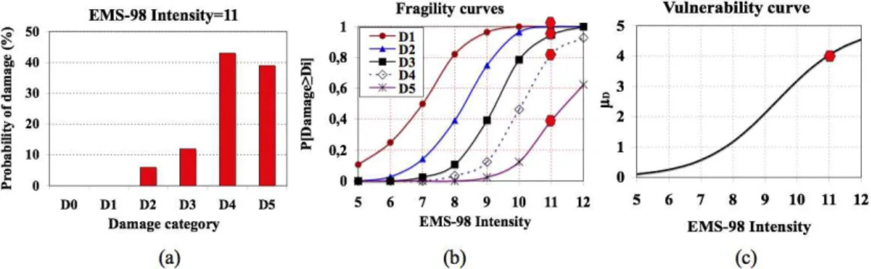
Fragility curves provide the probability of reaching or exceeding a given damage level as a function of the intensity of the hazard. They are usually modelled by lognormal functions (Fig. 2-b).

Vulnerability curves are relationships between the mean of damages for a given type of building and the value of the hazard intensity (Fig. 2-c). These values can be calculated with the fragility curves and Equation 1 (Lagomarsino and Giovinazzi (2006)).

Equation 1

µ

∑

where µD is the mean damage for a particular value of hazard intensity, Pk is the probability of a damage level Dk, and k is the range of the damage category (from 0 to 5 in the EMS-98 damage scale).

An example of these curves is shown in Fig. 2 for a massive stone masonry building (type M4) according to the EMS-98 (Lagomarsino and Giovinazzi (2006)). Fig. 2-a shows the damage distribution for this type of building for an earthquake intensity of 11. After calculating these damage distributions for all intensity levels, we can construct Fig. 2-b. Then, all this material is combined to calculate a mean damage value from Equation 1; thus, for each intensity level, we can plot the vulnerability curves shown in Fig. 2-c.

Fig. 2. Damage distribution (a), fragility curves (b) and vulnerability curves (c) for the M4 building type, according to EMS-98.(Saeidi et al. 2009)

In practical terms, when developed and validated, fragility and vulnerability curves are both efficient and accurate. Vulnerability curves are used to obtain a synthetic value of the mean damage to the buildings within a given territory, for each considered building type. When applied to a single building, fragility curves may be used to assess the probability of reaching a particular damage level. When applied to a set of buildings, fragility curves may be used to assess the damage distribution of all these buildings.

2.Methodology for the development of analytical vulnerability functions in subsidence area

The methodology adopted in this study to develop vulnerability and fragility curves is based on the damage assessment of a set of theoretical buildings whose characteristics are consistent with a particular building type, but are also variable in order to take into account both the variability of the type and the uncertainties. The method is based on four steps (Fig. 3).

The first step consists of preliminary choices regarding a damage scale, an intensity criterion and an analytical method for the building damage evaluation. These choices will be discussed in part 3, because they are highly dependent on the chosen analytical method, as will be described. A five-level damage scale is chosen, and the intensity criterion is the

horizontal ground strain parameter εground. The second step consists of defining a building typology and choosing the representative characteristics of each type.

The third and fourth step consist on a Monte Carlo simulation method. For each type, the third step consists of simulating a database of 1000 virtual buildings whose characteristics (e.g., height, length, materials, and mechanical properties) are consistent with the studied building type. This step is presented in section 4.1, where two building types are considered: unreinforced masonry buildings and reinforced masonry buildings.

The fourth step consists of evaluating the damage of the 1000 simulated buildings for one value of the intensity criterion and counting the number of buildings into each damage class. This leads to a graph similar to Fig. 2-a, and the results may then be used to plot a set of points for both the fragility curve (probability of reaching or exceeding a given damage class) and the vulnerability curve (mean damage). Finally, by repeating this step for all the values of the horizontal ground strain, both the vulnerability and fragility curves can be drawn. This step is discussed in sections 4.2 and 4.3.

The fifth step consists of fitting a mathematical model to the results in order to express the fragility and vulnerability as mathematical functions. A tangent hyperbolic function is used for the vulnerability functions, and a log-normal function for the fragility functions.

Fig. 3. Methodology for the determination of vulnerability and fragility curves in the subsidence zone. The issue of the building relative positions into the settlement through needs further clarification. Section 3 addresses the question of the development of vulnerability curves. These curves can be generated independently of any consideration about a particular event. However considerations about the location of each building in a subsidence through are necessary to assess the specific value of the horizontal ground strain in the vicinity of the building and apply these functions. This point is discussed in section 5, with the application and validation of the functions.

3.Preliminary choices

3.1.Choosing an analytical method for the evaluation of building damage in subsidence areas.

The first analytical method of building damage assessment was developed by Burland and Wroth (1974), and several extensions are now available (Boscardin and Cording, (1989); Boone, (1996); Burland, (1995); Boone, (2001); Finno et al. (2005)). In these methods, masonry buildings are modelled with an isotropic and elastic beam with two supports, loaded by a central or uniformly distributed load. A deflection ∆ is imposed on the beam to model the ground curvature that corresponds to the bending effect of the subsidence on the building (Fig. 4). The maximum tensile strains due to bending deformation and shear deformation are then calculated and compared with the values of the critical tensile strains for the determination of the damage class. All of the current analytical methods use five damage classes, and Table 1 gives the five damage classes defined by Burland (1995) and Boscardin and Cording (1989).

Fig. 4. Beam model for building in subsidence zone (after Burland et al. (2004)).

Differences between these methods concern the modelling of the subsidence effect, the loading distribution (building weight), the location of the neutral axis, the building type and the imposed relationships between the mechanical parameters:

(i) Most of the methods consider the deflection ∆ to model the effect of the subsidence. Boscardin and Cording (1989) extended the approach of Burland and Wroth (1974) by superimposing the horizontal strain εh induced by the horizontal ground strain onto those generated by the bending of the beam. These methods assume that the deflected beam is then also subjected to a uniform extension over its full depth. Consequently, both the deflection and the horizontal strain are intensity criteria (Kratzsch, (1983)). Nevertheless, taking two intensity criteria into account may appear difficult for the development of vulnerability functions that require the use of a single intensity criterion. Finally, investigations are made to justify mathematical relations between these two criteria, in relation to the mining and geological context, and these two criteria are reduced to one (see section 3.3).

(ii) Analytical methods consider different types of buildings. Burland and Wroth (1974), as well as Boscardin and Cording (1989), consider masonry buildings modelled with isotropic beams, and they suggest adjusting the ratio E/G of the Young’s modulus E to the shear modulus G of the beam to be between 2.4 and 12.5, in order to take into account the influence of the openings (doors and windows) that would cause an increase in the shear deformation. Son and Cording (2007) investigated the possible range of the E/G ratio in relation to the number of windows, and they show that this ratio may be close to 60. These values denote an anisotropic behaviour of buildings that is incompatible with the first assumption of an isotropic beam that imposes a E/G ratio between 2 and 3. Boone (1996, 2001) considers three types of buildings: load bearing wall masonry buildings, in-fill walls and beam-in-frame structures. Finno et al. (2005) suggest a model to take into account the positive influence of the concrete floors of buildings under study. The present paper addresses the question of the vulnerability functions of masonry buildings and the method chosen is based on the method of Burland (1995).

(iii) Burland (1995) considered both a uniformly distributed and a central point load to model the building weight. Boscardin and Cording (1989) and Finno et al. (2005) also considered the central load assumption, while Boone (1996, 2001) considered the uniformly distributed load assumption. In the present paper, we have selected a uniformly distributed load because it appears to be more realistic than the central point load assumption.

(iv) The localisation of the neutral axis is also a debatable question. In the hogging area, Burland and Wroth (1974) and Boscardin and Cording (1989) consider that the neutral axis is probably located at the bottom of the beam because of the small tensile resistance of the upper levels of the masonry building and the greater tensile resistance of the foundation level. Boone (1996) considers this to be debatable because of the influence of the floors and the roof that may increase the tensile resistance. In our case, we have assumed that the neutral axis is located in the middle, i.e., superimposed on the central axis.

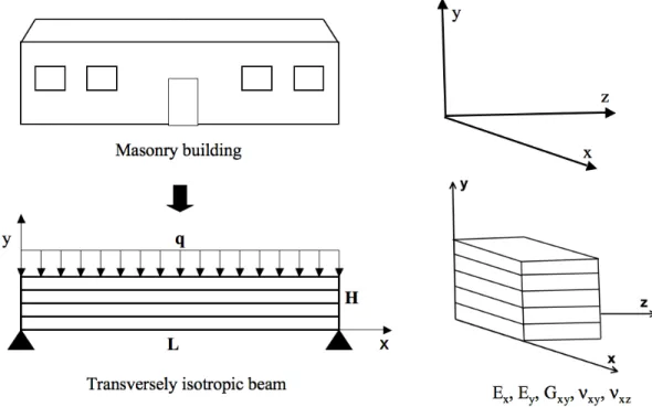
3.2.Details about the chosen analytical method for damage evaluation

The chosen method is mainly based on the Burland method (1995) and explicitly takes into account an anisotropic behaviour of buildings. The building is modelled as a transversely isotropic and elastic beam with two supports (Fig. 5): with a length of L, a height of H, a second moment of area I, and a uniform vertical load q that represents the building weight. The transversely isotropic behaviour is defined with 5 independents parameters. Two Young’s modulus Ex and Ey, two Poisson’s ratio νxy and νxz and one shear modulus Gxy (Fig. 5). Assumptions are made to reduce to 3 the number of independent parameters: Ex = Ey =E and νxy = νxz = ν.

Fig. 5. Transversely isotropic beam model for masonry building.

Two imposed movements are considered to model the effect of the mining subsidence. A vertical transmitted deflection ∆ is imposed at the centre of the beam to model the effect of the ground curvature, and a uniform horizontal transmitted strain εh is imposed to model the effect of the horizontal ground strain. Note that both ∆ and εh are dependent on the values of the free-field ground displacement and the stiffness of the building, because a rigid building may induce important soil-structure interactions that lead to reduced values of the transmitted displacements. This point is further addressed in section 3.3.

Based on the theory of Timoshenko (1957), Burland and Wroth (1974) identified two critical sections in the beam where maximal tensile strains will occur; the half span section and the edge section. In these two sections, the maximal tensile strain must be calculated in order to allow a comparison to threshold values associated with different damage classes. The relationships between ∆ and the maximum tensile strain εb in the half-span critical section, or the maximal diagonal tensile strain εd in the edge section, are calculated by

Burland (1995) according to Equation 2 and Equation 3, where y is the distance between the neutral axis and the lower fibre of the beam. No difference exists between the isotropic and the transversely isotropic models. Introduction of non-isotropic values of ν and E/G in Burland’s expressions can appear as an heuristic approach to take into account the real anisotropic behaviour of masonry walls. However, Equation 2 and Equation 3 remain similar for isotropic and transversely isotropic models if it is assumed that, the normal to centroidal axis remains normal and straight after bending. This assumption is confirmed by Hashin (1967) that investigated plane anisotropic beams and showed that the same equations can be used with accuracy for isotropic and anisotropic beams.

Equation 2 ∆ L = 5⋅L 48⋅y+ 3⋅I 2⋅y⋅L⋅H ⋅ E G      εb Equation 3 ∆ L = 1 2 + 5H⋅L2G 144⋅E⋅I      εd

The effect of the uniform horizontal transmitted strain εh, may then be added in order to calculate the maximal value of the principal tensile strain in the two critical sections.

In the half span critical section, both ∆ and εh induce principal horizontal tensile strains. The maximal tensile strain εbmax is then estimated as the sum of these two principal tensile strains (Equation 4):

Equation 4

ε

ε

ε

In the edge critical section, ∆ induces vertical shear stresses and ultimately a diagonal principal tensile strain, while εh induces a horizontal principal tensile strain. The maximal tensile strain εdmax is then evaluated using Mohr’s circle of strain (Equation 5, Burland et al. (2004)). Equation 5 εd max =εh( 1−ν 2 )± εh 2 (1+ν 2 ) 2+ε d 2

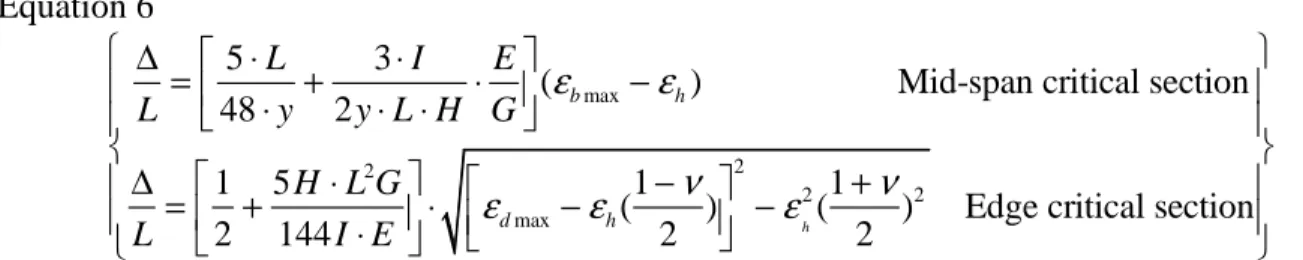
By substituting the values of εb in Equation 2 into Equation 4 and εd in Equation 3 into Equation 5, the relationship between the relative deflection parameter (∆/L), the transmitted horizontal strain (εh) and other building parameters is calculated for the two critical sections (Equation 6). The difference between the isotropic and the transversely isotropic models is important in the second expression of the Equation 6. For an isotropic beam, ν can be replaced by 2.E/G – 1 that leads to highly different results than when ν, E and G are independent.

Equation 6 ∆ L = 5⋅L 48⋅y+ 3⋅I 2y⋅L⋅H ⋅ E G     

(

ε

ε

∆ L = 1 2+ 5H ⋅L2G 144 I⋅E      ⋅

ε

ε

ν

ε

ν

Edge critical section              

Burland et al. (1977) defined the concept of limiting tensile strain εlim that must be compared to the maximal tensile strains εbmax and εdmax to define the threshold value of the maximal tensile strain before damage occurs. Like Boscardin and Cording (1989), Burland

et al. (1995) defined different threshold values for different damage levels according to

Table 1, and they considered these values for a large quantity of buildings. Most of the analytical methods use these thresholds values to assess the building damage, and we have also used the same values.

Table 1. Threshold values of the limiting tensile strain εlim associated with the five damage classes (Boscardin and Cording, 1989; Burland et al. (2004)).

Damage class Limiting tensile stain (εlim)%

D0 Negligible 0-0.05

D1 Very slight 0.05-0.075

D2 Slight 0.075-0.15

D3 Moderate 0.15-0.3

D4 and D5 Severe to Very Severe >0.3

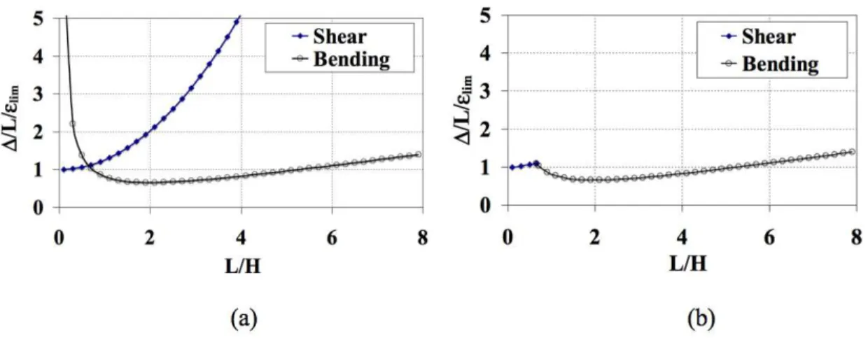
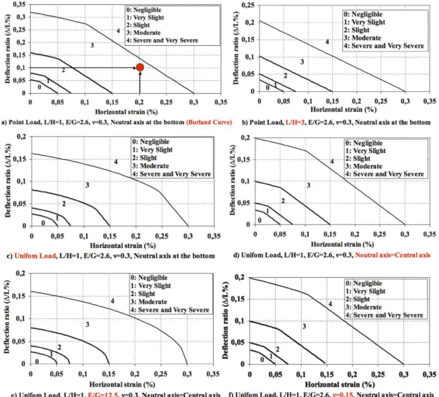
The two relations from Equation 6 are usually used to plot the ∆/(L.εlim) ratio versus the L/H ratio for given values of the building mechanical properties and the uniform horizontal transmitted strain εh. Fig. 6-a shows a result for the case where εh is set equal to 0, the E/G ratio is 2.6 (case of an isotropic beam with ν = 0.3) and the neutral axis is in the middle. This figure shows two curves: one is associated with the tensile strain due to shear near the edges of the beam (Fig. 4-d), and the other is associated with the tensile strain due to bending in the middle span of the building (Fig. 4-e). The minimum value of ∆/L/εlim between these two curves is a critical value, and it can be used to assess the maximal admissible relative deflection ∆/L. For a given value of the limiting tensile strain (εlim), the smallest value of ∆/L/εlim between the two curves indicates whether the failure will occur near the edge section (shear) or near the middle section (bending). It appears that for small values of the ratio L/H, failure will occur near the edge of the building where the maximal tensile strain due to shear first reaches the limiting value εlim. For greater values of the ratio L/H, failure will occur in the middle section (Fig. 6-b).

For given values of the building dimensions and mechanical properties, the two relations of Equation 6 are also used to plot the damage curves (Fig. 7), which are used to assess the damage level in relation to the horizontal strain and the building deflection.

Fig. 6. Limiting relationships between (∆/L)/εlim and L/H.

Fig. 7 shows the damage curves for different sets of parameters. Fig. 7-a shows the original Burland (1995) curves for a point loaded beam with L/H=1, E/G=2.6, υ=0.3 and the neutral axis in the bottom of the beam. A circular dot is plotted in order to illustrate the use of these curves. In the case of ∆/L = 0.1% and εh = 0.2%, the damage is moderate. The discontinuity of the damage curves is a consequence of the transition between the failure mode-) associated with the critical section where εbmax or εdmax first reach the value of εlim. Fig. 7-b considers the same parameters, but the L/H ratio is set to 3. In this case, the curves do not show any discontinuity, and the failure always occurs in the middle critical section. A comparison of the two figures (Fig. 7-a and Fig. 7-b) shows that buildings with L/H=3 are more vulnerable than buildings with L/H=1.

Fig. 7-c investigates the effect of a uniform vertical load and considers the same parameters as Fig. 7-a. The results show that the central point load assumption is not conservative. For this reason, and because the uniformly distributed load is more realistic, the assumption of a uniformly distributed load is justified in the proposed methodology.

Fig. 7. Damage identification curves for buildings according to the Burland (1995) method.

Fig. 7-d investigates the influence of the neutral axis localization. A comparison with Fig. 7-c shows that the bottom assumption is more conservative. Nevertheless, because the differences are small and because the relevance of this assumption is debatable (Boone 1996), we prefer the assumption that the neutral axis is set in the middle of the beam. Fig. 7-e investigates the influence of the E/G ratio for an transversely isotropic beam with

υ=0.3. The comparison with Fig. 7-d shows important differences regarding the global shape that reveal the importance of this parameter.

Fig. 7-f investigates the influence of the Poisson’s ratio, used in Equation 6. A comparison with Fig. 7-d shows that the model is not much sensitive to this parameter.

All these comparisons demonstrate that none of these damage curves are suitable for all buildings, and that it is important to calculate and use the correct damage curve associated with the most realistic building parameters.

3.3.Determination of an intensity criteria in subsidence areas

The use of an analytical method to develop vulnerability functions raises two difficulties in addition to the definition of the analytical method.

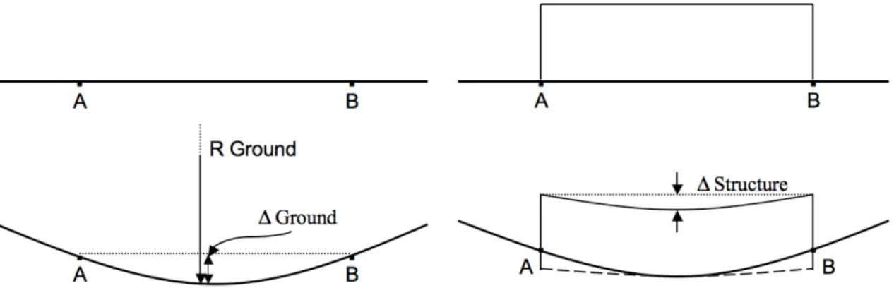
(i) First, the chosen analytical method uses the values of the building induced movement that may be significantly different than the values of the free-field ground movement that would take place without any structure (Fig. 8). These differences are the consequence of complex soil-structure interaction phenomena that lead to a transmitted value that may be drastically reduced compared to the field ground movement. Nevertheless, the free-field ground movements appear to be relevant for the choice of intensity criteria because they characterize the subsidence, while the transmitted ground movements characterize both the subsidence and the soil-structure interactions. Several studies can be used to predict the free-field ground movements (NCB, 1975; Kratzsch, 1983). If ∆ground and εground are the free-field ground displacements, two coefficients must be defined to quantify the transmitted movements ∆structure and εstructure (Equation 7).

Fig. 8. Deflection parameter for ground and structure. (Left) – case without structure. (Right) -case with a structure and influence of the soil-structure interaction.

Equation 7 εstructure =

K_ε⋅ε_ground

∆_structure= K_∆⋅ ∆_ground

The determination of K∆ and Kε is difficult, and it depends on the soil and the mechanical

characteristics of the building. Boscardin and Cording (1989) and Potts and Addenbrooke (1997) investigated this question for a large range of buildings. For masonry buildings with dimensions and properties equivalent to those defined in Table 2, and for a Young’s modulus of the ground between 50 to 300 MPa, the value of Kε may vary between 1 and 30% in relation to the building stiffness, and K∆ may vary between 20 and 70 %.

(ii) Second, it has been shown that the chosen analytical method is based on two intensity criteria: the building deflection and the transmitted horizontal strain. However, the vulnerability functions are based on the use of unique intensity criteria. Moreover, most empirical methods for building damage assessment in a subsidence area are based on the

1988). Consequently, the free-field horizontal ground strain appears to be the most efficient choice for the intensity criteria. This choice raises the question of the relationship between the free-field horizontal ground strain and the ground deflection.

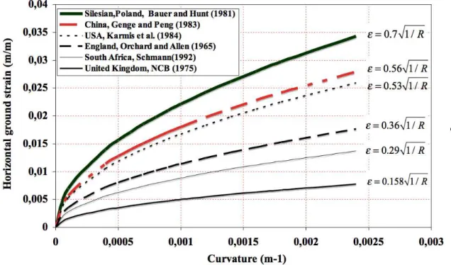
According to the empirical studies from different countries for different geological contexts and both longwall and room and pillar mining methods (Karmis et al. (1984), Orchard and Allen 1965), a relation between the free-field horizontal ground strain εground and the ground radius of curvature Rground can be defined according to Equation 8 (Fig. 9).

Equation 8

εground = Ksite 1 / Rground

Ksite is a coefficient that probably depends on the geological and mining context (mining method, mine geometry, overburden, …) but no studies have investigated this point and its determination is mainly based on empirical data (Fig. 9).

Fig. 9. The values of Ksite parameter in different regions.

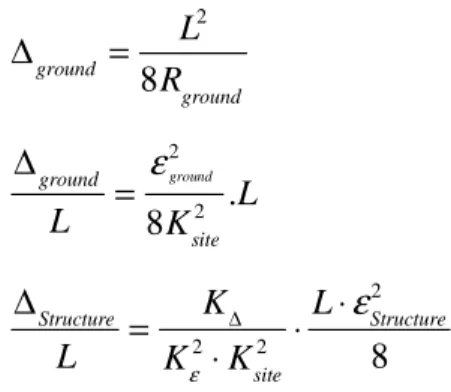
Moreover, in the case of mining subsidence, the building length is mostly smaller than the subsidence dimensions and the ground curvature may be assumed constant over the building. It is then possible to calculate (beam theory) the geometric relationship between the ground curvature and the ground deflection, using the building length L and considering a circular shape for both the ground and building final curvature (Kratzsch, 1983; Burland and Wroth, 1974; Burland et al., 1977, Equation 9). By substituting Equation 9 into Equation 8, the relationship between the ground deflection and the horizontal ground strain is obtained (Equation 10). Then, by substituting Equation 10 into Equation 7, the relationship between the building deflection and the horizontal structure strain is obtained (Equation 11).

Equation 9 ∆_ground = L2 8R_ground Equation 10 ∆_ground L =

ε

ε

4.Application of the methodology for developing vulnerability and fragility curves 4.1.Choice of a building typology and construction of a database of virtual buildings

The methodology used to develop the vulnerability and fragility curves is described in Fig. 3. The first step is presented in section 3. The free-field horizontal ground strain is chosen as the intensity criteria, and the analytical method is based on the Burland method (1995). The next steps of the methodology show that each vulnerability curve is associated with a building type. In this study, two masonry building types are investigated, with the same geometric parameters (L, H) taken into consideration. Unreinforced masonry buildings (URM) that are moderately rigid are considered first, and more rigid reinforced masonry buildings (RM) are considered second. Three parameters are directly related to the building stiffness. For the RM buildings, the E/G is considered to be smaller than for the URM buildings (Burland 1995). In addition, the two parameters K∆ and Kε are smaller for the

rigid buildings because of the increase in the soil-structure interaction phenomena (Potts and Addenbrook, 1996). A discussion of the determination of these important parameters is not within the scope of this research. Their determination for the two building types is based on the results of Boscardin and Cording (1989) and Potts and Addenbrook (1996). Table 2 describes the two building type, where each parameter is variable because of the variability of the buildings within the same type due to real physical and observed differences between the buildings. Moreover, this table also takes into account uncertainties concerning their true characteristics.

Length and height are chosen to be representative of the buildings in many mining regions, particularly the Lorraine region.

Variability of the E/G ratio is estimated from the numerical results of Son and Cording (2007), who have investigated the equivalent stiffness of masonry buildings with a distinct element method. Regarding the masonry buildings in France and in many countries, the percentage of the open surface for the two types of masonry buildings is considered between 10 to 20%. The E/G ratio for the RM buildings (between 2 and 5) is in accordance with results obtained for a wall with equivalent shear and normal stiffness of the joints, while for the URM buildings, the E/G ratio (between 10 and 15) is relevant for a wall with a joint shear stiffness up to twenty times smaller than the joint normal stiffness.

The Poisson’s ratio, used to calculate the maximal tensile strain on the edge critical section of the beam (Equation 6), has a small variability: 0.2 to 0.3. These values are in global agreement with experimental studies on masonry mechanical behaviour (Lourenco and Rots, 1993).

Table 2 is used to develop a representative database of each building type with 1000 simulated buildings. To complete this database, the variability of all the parameters is considered in agreement with the building type. Each building is then characterized by random values that are consistent with uniform probability distributions over the ranges indicated in Table 2. After preliminary tests from 100 to 5000 rows, 1000 rows has proven to provide acceptably accurate results for the final vulnerability curves.

Table 2. Variability of the parameters for the two building types used in simulating a database of virtual buildings.

Building Soil and soil structure interaction coefficients

B u il d in g ty p e L en g th [ m ] H ei g h t [m ] L /H E /G ν Ksi te K∆ Kε Unreinforced Masonry (URM) 20-30 7-10 2-4.2 10-15 0.2-0.3 0.1 - 0.2 40 - 70% 10 - 30% Reinforced Masonry (RM) 20-30 7-10 2-4.2 2-5 0.2-0.3 0.1 - 0.2 20 - 50% 1 à 20%

4.2.Development of vulnerability functions

According to Fig. 3, the fourth step of the methodology is the damage assessment for all 1000 simulated buildings and for different values of the horizontal ground strain. Calculations are performed with Mathematica software (Wolfram, 2007) in which the analytical method is implemented. Because of the parameter variability, not all the buildings suffer the same damage for a given value of horizontal ground strain. Vulnerability curves for a given building type show the relationship between the mean damage and the horizontal ground strain. The mean damage is calculated from Equation 12. Equation 12

µ

ε

∑

∑

µD(ε) is the mean damage for the value εground of the horizontal ground strain, N(Di) is the number of buildings in the damage class Di among the 1000 simulated buildings, and P(Di) is the percentage of the 1000 buildings with a damage of Di.

Vulnerability curves may then be modelled in order to obtain a vulnerability function. The tangent hyperbolic function is often used in other fields (Lagomarsino et al. (2006)), according to Equation 13.

Equation 13 µD(ε)=a[b+Tanh(c⋅ε+d )]

where µD(ε) is the mean damage for a value εground of the horizontal ground strain, and a, b, c, and d are four coefficients that must be determined for each building type. For example the vulnerability curves for the two building types describe in Table 2 are shown in Fig. 10. The equations of the fitted curves for these two buildings types are:

For URM type:

µ

ε

ε

µ

ε

ε

Fig. 10. Vulnerability curves and functions for the URM and RM building types.

Comparison of vulnerability curves in Fig. 10 shows that for each value of the horizontal ground strain, the mean damage for the reinforced masonry buildings (RM) is less than that for the unreinforced masonry buildings (URM). This is consistent with the fact that the URM buildings are more vulnerable compared to the RM buildings.

4.3.Sensitivity analysis

A sensibility analysis is performed to investigate the influence of each parameter. Values of the URM building parameters are chosen for the reference case of the analysis. Value of each parameter is then modified so that the mean value is multiplied or divided by a two factor with a constant range of variation (Table 3). For the parameter E/G, two ranges are investigated. One that corresponds to a division by a two factor, and another that corresponds to an isotropic behaviour.

Table 3. Variability of the parameters for the sensibility analysis. Reference case Investigated values

E/G 10-15 4-8 or 0.5-2.6 Ksite 0.1 - 0.2 0.25 – 0.35

Kε 10 - 30% 30 – 50%

K∆ 40 - 70% 10 – 40%

Results of the sensibility analysis are shown in Fig. 11. Effect of parameters Ksite, Ke and KD appears more important than the effect of other parameters. The building vulnerability increases when increasing the value of Kε, K∆ and E/G. On the contrary the building vulnerability decrease when Ksite and L/H increase.

Influence of Kε, K∆ and Ksite is logical. The value of the transmitted horizontal strain and deflection increase with Kε and K∆ (Equation 7). Moreover, Equation 10 shows that for a given value of εground, the ground deflection and the final building deflection decrease when Ksite increases.

Influence of the parameter E/G is really more complex and depends on the value of L/H. For small values of L/H, the maximal strain is more likely to occur in the edge critical section (Fig. 6). Second part of Equation 6 must then be used and it can be observed that

εdmax increases with increasing E/G. On the contrary, for large values of L/H, the maximal strain occurs in the mid-span critical section (Fig. 6). First part of Equation 6 must then be used and it can be observed that εbmax decreases with increasing E/G.

Exact influence of L/H is also more complex. In particular, Fig. 6 shows that the building vulnerability may reach a maximum for a particular value of L/H (L/H = 2 with the example of Fig. 6).

Fig. 11. Sensibility analysis for the different parameters used to calculate the vulnerability curves.

4.4.Development of fragility curves

Fragility curves show the relationship between the value of the horizontal ground strain

εground and the probability of reaching or exceeding a given damage level for a given building. This probability is calculated with Equation 14.

Equation 14 P( Damage≥D_i)=1− N ( DJ) n J=1 i−1

∑

∑

where P(Damage ≥ Di) is the cumulative probability that the damage level exceeds Di ; N(Dj) is the number of buildings in the damage class Dj among the 1000 simulated buildings; and n is the total number of simulated buildings (n=1000). P(DJ) is the percentage of the 1000 buildings whose damage is Dj. Results are shown in Fig. 12 for the two building types. These results show that, the cumulative probability P(Damage ≥ Di) is greater for the URM building type than for the RM type.

Fig. 12. Fragility curves for the URM and RM building types.

5.Application and validation of vulnerability curve 5.1.Application of vulnerability curves

When developed, vulnerability curves can be applied to assess building damage due to a future possible subsidence. The first step is the prediction of the subsidence parameters at the ground surface: vertical subsidence and horizontal ground displacements. Many methods exist that are not into the scope of this paper (Whittaker and Reddish (1989), Melis

et al. (2002) and Coulthard et al. (1998)). The second step is the calculation of the

horizontal ground strain at the ground surface, in the vicinity of each building. Building damage can then be assessed by the use of vulnerability curves.

Many uncertainties generally affect the estimation of the horizontal ground strain. Some simplifications are then possible and a zoning of the horizontal ground strain can be considered.

In all cases, vulnerability curves must be carefully used. Estimated damage is not the damage of the building, but the mean of damage. When applied to a single building, this damage can be considered as the most probable damage. When applied to a group of buildings of the same type affected by a roughly similar horizontal ground strain, this damage can be considered as the mean value of the damage of each building.

5.2.Validation of methodology with observed damage in masonry buildings in the Lorraine region

In France, the Lorraine region features large quantities of iron, salt, and coal deposits that were heavily extracted until the beginning of the 1990s (salt is still mined). The local French administration estimates that 140 square kilometres of land surface are undermined, most of this area comprising abandoned mines that have causes extensive underground cavities.

Between 1996 and 1999, five accidental subsidence events occurred, 30 to 50 years after the extraction stopped (two in the city of Auboué in 1996, two in Moutier in 1997, and the last one in Roncourt in 1999) and caused damage to more than 500 dwellings (Deck, (2002)). Many other cities and villages in Lorraine may still be affected by this phenomenon.

Information about the damage of each building in relation to its geometrical and architectural characteristics and the horizontal ground strain in its vicinity has been collected for three of these events (Roncourt, Moutier-Haut and Moutier-Stade). Among all the buildings located in the subsidence areas, a set of 178 buildings of two types have been selected. These types consist of unreinforced masonry buildings (URM1) and reinforced masonry buildings (RM1) with lengths between 10 to 20 m, heights between 4 and 8 m and other characteristics presented in Table 4. The Ksite parameter in Lorraine is estimated to be

0.1 to 0.2 (Al Heib, 2002; Deck, 2002) and the two parameters K∆ and Kε are estimated

from Boscardin and Cording (1989) and Potts and Addenbrook (1997). Final values are similar to those adopted in the previous section (Table 2).

Table 4 summarizes the variability of the parameters that characterize the two building types URM1 and RM1 in Lorraine. The vulnerability curves of the two building types are calculated with the method described above. Empirical data are then used to compare these curves with damage observations.

Table 4. Variability of the parameters for the buildings in the Lorraine region. Initial values for URM1 and RM1 are those usually found in literature. Adjusted values for URM1 and RM1 are obtained after comparing

vulnerability curves and empirical data.

Dat a are 178 buil din gs dam age d in the cities of Roncourt, Moutier-Haut and Moutier-Stade. Damage of each building has been assessed in detailed reports made by experts from governmental administrations and insurance companies. The main difficulty is the calculation of the horizontal ground strain in the vicinity of each building. An extensive monitoring was implemented, but only the vertical subsidence is satisfactorily known. The horizontal ground strain is dependent on the ground curvature (Fig. 9) and its typical profile is shown in Fig. 13. Empirical equations suggested in the literature (Whittaker and Reddish (1989)) are used to identify the location where the horizontal strain is maximal, i.e. approximately the quarter of the distance between the inflection point and the centre or the border of the subsidence profile. Consequently, for each building, a semi section of the vertical subsidence is plotted and three points are identified (Fig. 13): C is the centre of the subsidence, I is the inflexion point of the profile and B is its border.

Building Soil and soil structure Interaction

Coefficients Building type _Len g th [m ] H ei g h t [m ] L /H E /G ν Ksi te K∆ Kε URM1 10-20 4-8 1.25-5 10-15 0.2-0.3 0.1 - 0.2 40 - 70% 10 - 30% RM1 10-20 4-8 1.25-5 2-5 0.2-0.3 0.1 - 0.2 20 - 50% 1 - 20% URM1 adjusted 10-20 4-8 1.25-5 10-15 0.2-0.3 0.1 - 0.2 50 - 70% 35 - 45% RM1 adjusted 10-20 4-8 1.25-5 2-5 0.2-0.3 0.1 - 0.2 30 - 50% 10 - 20%

Fig. 13. The method of calculation of horizontal ground strain in each building.

The horizontal ground strain profile is linearized and the horizontal strain amplitude SAM is assessed with a value between 0 and 1. SAM is then multiplied by the maximal value of the horizontal ground strain (Equation 15, Whittaker and Reddish (1989)).

Equation 15 ε_Max = K SMax

H

where SMax is the maximum vertical subsidence, H is depth of the mine or excavation and K is a coefficient that must be determined for each mining region. In the Lorraine region, K is between 1 and 1.5 (Al Heib (2002)) and a value of 1.25 is considered.

The data regarding the damage (value between 0 and 4) and the horizontal ground strain are summarized in Table 5. Six ranges are considered for the horizontal ground strain. For each range, the number of concerned buildings Nb is used to calculate the mean value of the damage µD and of the strain µε.

Table 5. Synthesis of damage observed in the Lorraine region (France) for three critical subsidence events. The mean value of damage and of the strain is calculated in order to compare observations with analytical

vulnerability curves.

Moutier-Haut Moutier-Stade Roncourt

εground [mm/m] µε [mm/m] µD Nb εground [mm/m] µε [mm/m] µD Nb ε ground [mm/m] µε [mm/m] µD Nb ≤2 1 1.3 34 ≤2 1 1.5 40 ≤2 1 0.93 14 2-4 2.9 2.43 14 2-4 3 1.7 15 ≥2 3.4 1.6 13 4-6 4.9 3.63 8 4-6 4.3 2.3 7 6-8 7 3.6 5 8-10 9 3.5 12 ≥10 12 3.4 16

Results are then compared with vulnerability curves in Fig. 14-a. This comparison shows that there is good agreement between the building damage data in Lorraine and the calculated vulnerability curves. Nevertheless some differences exist for the smallest and largest values of the horizontal ground strain. The vulnerability functions underestimate the damage for the smallest values of the horizontal ground strain (less than 3 mm/m) and overestimate the damage for the greatest values (greater than 9 mm/m). One possible explanation of these differences is the existence of preliminary building damage due to building aging and other building pathologies (e.g., settlement during construction). For the greatest values of the horizontal ground strain, the overestimation of the damage shows that there are always some building types that are stronger than the predicted resistance.

Moreover, differences between the data and the vulnerability functions in Fig. 14-a may also be a consequence of the uncertainties regarding the values of the two soil-structure interaction parameters: K∆, Kε. A retrospective analysis is performed in order to find the

best values of these two parameters. Final values are greater than initial values (Table 4 for adjusted RM1 and URM1). This means that the real transmission ratio of the ground movements is probably greater than the predicted ratio. Fig. 14-b shows a comparison between the building damage data and the adjusted vulnerability curves.

In conclusion, the methodology for the determination of vulnerability curves is efficient for the prediction of building damage in a subsidence zone. A key point of the method is the choice and the justification of the soil-structure interaction parameters that must be specifically defined for each mining and building context.

Fig. 14. Vulnerability curves for reinforced and unreinforced masonry buildings in Lorraine, and a comparison with observed damage data in three cities (Moutier-Stade, Moutier-Haut and Roncourt). (a) preliminary vulnerability curves with initial values of the soil-structure interaction parameters K∆, Ke. (b)

6.Conclusion and perspectives

This paper has investigated a method for the development of vulnerability and fragility curves based on the use of analytical methods already developed and used for the damage assessment in mining subsidence areas.

The analytical method of Burland (1995) has been used for damage assessment in relation to the horizontal strain and the deflection transmitted to buildings. An transversely anisotropic behaviour is considered so that buildings are characterized by three independent parameters. Three coefficients (Ksite, K∆, Kε) have been used to estimate the strain and deflection from the free-field horizontal ground strain. Ksite is a characteristic of the mining and geological context of the studied area, while K∆ and Kε are characteristics of the soil-structure interaction, and depend on the difference in stiffness between the ground and the building. Realistic values of these coefficients have been suggested based on the research of Boscardin and Cording (1989) and Potts and Addenbrook (1996).

Damage curves were plotted, in addition to the damage curve of Burland (1995), in order to investigate the influence of the geometrical and mechanical parameters of the buildings. The L/H and E/G ratios both appeared to have a significant influence.

Vulnerability and fragility curves are efficient methods for the assessment of building damage. They also take into account uncertainty in the assessment process. Their use allows the probability to reach or exceed any given damage level for assessment. Therefore, they constitute an important extension of the existing methods for the damage assessment in mining subsidence hazard areas. The Mont Carlo simulation method was used to develop the vulnerability functions with a database of 1000 simulated buildings whose parameters are randomly chosen within their possible range of variation for each building type.

Vulnerability and fragility curves have been developed for two building types that are typical of a large number of countries: unreinforced masonry buildings and reinforced masonry buildings with lengths between 10 and 20 meters and heights between 7 and 10 meters. Three ranges of variation have also been investigated for the Ksite parameter, in order to increase the number of sites where the developed curves may be used for operational assessment of the building damage.

Finally, the methodology is applied in the French region of Lorraine, where mining subsidence hazard is a concern. Two specific vulnerability curves are calculated and compared to the damage observed after 3 mining subsidence events. The results showed good agreement between the theoretical and observed damage.

This research will be put into practise for the assessment of building damage that may occur over a large number of abandoned iron-mines in Lorraine. Almost 90% of the buildings can be classified into a set of about ten building types. Damage results will then be useful to define a better strategy for risk mitigation.

The methodology used to develop vulnerability functions could probably be used to develop vulnerability functions in the case of tunnelling induced ground movement, but with some modifications. In particular, this would require reconsidering relations between

the horizontal ground strain, the ground curvature and the deflection, in relation to the building length and the subsidence dimensions.

7.References

Al Heib M. (2002). Predicting the consequences of mines subsidence in Lorraine ferriferous region, Nancy, INERIS, INERIS-DRS-02-26146/RN02 for Geoderis.

Bauer R. A, Hunt S. R (1981). Profile , strain, and time characteristics of subsidence from coal mining in Illinois. Workshop on surface subsidence due to underground mining, Morgantown, West Virginia.

Boone S.J. (1996). Ground-movement related building damage. J. Geotech. Engng ASCE 122, No. 11, 886-896.

Boone S.J. (2001). Assessing construction and settlement-induced building damage: a return to fundamental principles, Proc. underground construction, institution of mining and metallurgy, London, 559-570.

Boscardin M. D, Cording E. J. (1989). Building response to excavation – induced settlement. J. of Geotechnical Engineering, 115, 1-21.

Burd, H. J., Houlsby, G. T., Augarde, C. E. (2000). Modelling tunnelling-induced settlement of masonry buildings. Proc. Instn Civ. Engrs Geotech. Engng, 143, 17-29.

Burland J. B., Wroth C. P. (1974). Settlement of buildings and associated damage. Conf. settlement of structures, 611-654.

Burland J. B., Broms B. B. et De Mello V. F. B. (1977). Behaviour of foundations and structures. 9th Int.conf. on soil mechanics and foundations engineering, Tokyo 2, 495-546.

Burland J.B. (1995). Assessment of risk of damage to building due to tunnelling and excavation. Proc. 1st Int. Conf. Earthquake Geotechnical Engineering, Ishihara(ed.),

Balkema, 1189-1201.

Burland J.B., Mair R.J and Standing J.R. (2004). Ground performance and building response due to tunnelling. Advance in geotechnical engineering, the skempton conference, 1, 291-342.

Carlos E, Ventura WD, Liam F, Onur T, Blanquera A, Rezai M. (2005). Regional seismic risk in British Colombia-Classification of buildings and development of damage probability functions. Canadian journal civil engineering 32, 372-387.

Coulthard M.A, Dutton A.J. (1998). Numerical modelling of subsidence induced by underground coal mining. The 29th U.S. Symposium on Rock Mechanics (USRMS),

Minneapolis, MN.

Deck O. (2002). Study of the effects of mining Subsidence on the structures, Phd thesis,

Franzius J.N., Potts D.M. and Burland J. B. (2006). The response of surface structures to tunnel construction. Proceedings of the institution of civil engineers. Geotechnical Engineering 159, 3-17.

Finno R.J. , Voss F.T., Rossow E., Tanner B. (2005). Evaluating Damage Potential in Buildings Affected by Excavations, Journal of Geotechnical and Geoenvironmental Engineering 131, No. 10, 1199-1210.

Geng D.Y and Peng S.S (1983). Long wall mining techniques for minimizing surface structural damage. SME-AIME Annual Meeting, Atlanta, Georgia, March 6-10.

Grunthal G. (1998). European Macroseismic Scale. Centre Européen de Géodynamique et de Séismologie, Luxembourg. Vol. 15.

Hashin ZVI. (1967). Plan Anisotropic Beams. Journal of applied mechanics. No

67-APM-7, 257-262.

HAZUS. (1999) Multi-hazard Loss Estimation Methodology Earthquake Model, Technical and User Manuals. Federal Emergency Management Agency, Washington, DC., chapter 2.

Karmis M., Triplett T. and Schilizzi P. (1984).- Recent developments in subsidence prediction and control for the eastern U.S. coalfield. 25 th. Symp. on rock mechanics,

713-913.

Kircher CA, Nassar AA, Kuster O, Holmes WT. (1997). Development of building damage functions for earthquake loss estimation. Earthquake Spectra, 13(4), 663-682.

Kratzsch H. Mining Subsidence Engineering. Springer-Verlag 1983.

Lagomarsino S, Giovinazzi S. (2006). Macroseismic and mechanical models for the vulnerability and damage assessment of current buildings. Earthquake Engineering , 4,

415–443.

Lourenco, P. B and Rots J. G (1993). On the use of micro-models for the analysis of masonry shear walls. The 2nd _{international symposium on computer methods in structural} masonry, 14-26.

Melis A., Medina L. and Rodríguez J.M. (2002). Prediction and analysis of subsidence induced by shield tunnelling in the Madrid Metro extension. Can. Geotech. J. 39(6), 1273–

1287.

McGuire R. K. (2004). Seismic Hazard and risk analysis. EERI Earthquake Engineering research Institute.

National Coal Board. (1975). Subsidence engineering handbook. chapter 6, 45-56.

Orchard R.J., Allen W.S. (1965). Ground curvature due to coal mining. Chartered Surveyor, 97, 622-631.

Potts, D. M, Addenbrooke, T. I. (1997). A structure’s influence on tunnelling-induced ground movements, Proc. Incln. Civ. Engng, 125, 109 - 125.

Ronald T. E, Hope A. S. (2008). Loss Estimation models and metrics. Risk Assessment, modeling and Decision Support. 135-157

Saeidi A., Deck O., Verdel T., (2009) Development of vulnerability functions in subsidence regions from empirical methods. Engineering structure Journal,

doi:10.1016/j.engstruct.2009.04.010.

Schümann E. H. R. (1992).- Occurrence of controlled coalmining subsidence in South Africa. COMA, Symposium on Construction over mined areas, South Africa, pp. 87-96.

Selby, A. R. (1999). Tunnelling in soils – ground movements, and damage to buildings in Worington, UK. Geotechnical and Geology Engineering 17, 351-371.

Skempton A.W, MacDonald D. H. (1956). Allowable settlement of building. Proc. INSTN. Civ. Engrs, 3, No.5, 727-768.

Son M. and Cording E.J. (2005). Estimation of building damage due to excavation-induced ground movements. Journal of Geotechnical and Geoenvironmental Engineering, 131, No.

2, 162-177.

Son M., Cording J. (2007). Evaluating of building stiffness for building response analysis to excavation-induced ground movements, Journal of Geotechnical and Geoenvironmental Engineering, 133, No. 8, 995-1002.

Son M., Cording J. (2008). Numerical model tests of building response to excavation-induced ground movements, Canadian Geotechnical Journal, 45, 1611-1621.

Spence R. J. S, Kelman I., Baxter P.J, Zuccaro G., Petrazzuoli S. (2005). Residential building and occupant vulnerability to tephra fall. Journal of Natural Hazards and Earth System Sciences 5, 477-494.

Timoshenko S. (1957). Strength of material-part I, D van Nostrand Co, Inc. London.

Wagner H, Schümann EHR. (1991). Surface effect of total coal seam extractions by underground mining methods. J.S.Afr.Inst.Min.Metal, 91, 221-231.

Whittaker B. N., Reddish D. J. (1989).- Subsidence : Occurrence, Prediction, Control.

Elsevier.

Wolfram S. (2007). Mathematica software version 6. Wolfram Research, Inc., USA.

Yu Z., Karmis M., Jarosz A., Haycocks C. (1988) Development of damage criteria for buildings affected by mining subsidence. 6th annual workshop generic mineral technology centre mine system design and ground control, 83-92.