Environmental Protection, Consumer Awareness, Product Characteristics, and Market Power

Texte intégral

(1)2007s-05. Environmental Protection, Consumer Awareness, Product Characteristics, and Market Power Marcel Boyer, Philippe Mahenc, Michel Moreaux. Série Scientifique Scientific Series. Montréal Mars/March 2007. © 2007 Marcel Boyer, Philippe Mahenc, Michel Moreaux. Tous droits réservés. All rights reserved. Reproduction partielle permise avec citation du document source, incluant la notice ©. Short sections may be quoted without explicit permission, if full credit, including © notice, is given to the source..

(2) CIRANO Le CIRANO est un organisme sans but lucratif constitué en vertu de la Loi des compagnies du Québec. Le financement de son infrastructure et de ses activités de recherche provient des cotisations de ses organisations-membres, d’une subvention d’infrastructure du Ministère du Développement économique et régional et de la Recherche, de même que des subventions et mandats obtenus par ses équipes de recherche. CIRANO is a private non-profit organization incorporated under the Québec Companies Act. Its infrastructure and research activities are funded through fees paid by member organizations, an infrastructure grant from the Ministère du Développement économique et régional et de la Recherche, and grants and research mandates obtained by its research teams. Les partenaires du CIRANO Partenaire majeur Ministère du Développement économique, de l’Innovation et de l’Exportation Partenaires corporatifs Alcan inc. Banque de développement du Canada Banque du Canada Banque Laurentienne du Canada Banque Nationale du Canada Banque Royale du Canada Banque Scotia Bell Canada BMO Groupe financier Bourse de Montréal Caisse de dépôt et placement du Québec DMR Conseil Fédération des caisses Desjardins du Québec Gaz de France Gaz Métro Hydro-Québec Industrie Canada Investissements PSP Ministère des Finances du Québec Raymond Chabot Grant Thornton State Street Global Advisors Transat A.T. Ville de Montréal Partenaires universitaires École Polytechnique de Montréal HEC Montréal McGill University Université Concordia Université de Montréal Université de Sherbrooke Université du Québec Université du Québec à Montréal Université Laval Le CIRANO collabore avec de nombreux centres et chaires de recherche universitaires dont on peut consulter la liste sur son site web. Les cahiers de la série scientifique (CS) visent à rendre accessibles des résultats de recherche effectuée au CIRANO afin de susciter échanges et commentaires. Ces cahiers sont écrits dans le style des publications scientifiques. Les idées et les opinions émises sont sous l’unique responsabilité des auteurs et ne représentent pas nécessairement les positions du CIRANO ou de ses partenaires. This paper presents research carried out at CIRANO and aims at encouraging discussion and comment. The observations and viewpoints expressed are the sole responsibility of the authors. They do not necessarily represent positions of CIRANO or its partners.. ISSN 1198-8177. Partenaire financier.

(3) Environmental Protection, Consumer Awareness, Product Characteristics, and Market Power* Marcel Boyer†, Philippe Mahenc‡, Michel Moreaux§ Résumé / Abstract Nous étudions le comportement d'un monopole dont la production cause un dommage global de pollution pour les consommateurs et les non-consommateurs de son produit et un dommage spécifique additionnel pour les consommateurs. Le monopole anticipe de manière stratégique l'impact des caractéristiques et du prix du produit et celui du niveau de pollution sur les décisions d'achat des consommateurs. Nous comparons le monopole standard non réglementé et le monopole sujet à une réglementation environnementale. Nous montrons que les deux monopoles choisissent la même variété de produit, que le monopole réglementé pollue moins, produit autant sinon plus, et demande un prix plus élevé que le monopole non-réglementé. Ainsi, la réglementation environnementale dans ce contexte entraîne toujours une hausse de prix mais ne mène jamais à une baisse de production. Mots clés : protection environnementale, consommateurs verts, caractéristiques des produits, pouvoir de marché. We investigate the behavior of a polluting monopolist whose production causes a global damage affecting consumers and non-consumers alike while consumption causes a specific damage affecting consumers only. The monopolist anticipates strategically how her decisions on product variant, price and pollution affect the purchasing decisions in a Hotelling market. We compare a standard unregulated monopolist and a monopolist subject to environmental regulation. We show that both monopolists choose the same product variant, that the regulated monopolist pollutes less, produces as much or more, and charges a higher price than the unregulated one. Hence, environmental regulation always lead to an increase in price but never to a reduction in production.. Keywords: environmental protection, consumer awareness, product characteristics, market power *. We thank Bernard Caillaud, Philippe Bontems and an anonymous referee for their comments. Financial support from CIRANO (Canada), CNRS (France) and INRA (France) is gratefully acknowledged. We remain of course solely responsible for the content of this paper and of its shortcomings. This paper has appeared in Boyer, M., Hiriart, Y. and D. Martimort (editors), Frontiers in the Economics of Environmental Regulation and Liability, Ashgate Pub., 2006 (pp. 121-151). † Bell Canada Professor of Industrial Economics, Department of Economics, Université de Montréal, CIRANO and CIREQ Fellow. Address: CIRANO, 2020 rue University, bureau 2500, Montréal (Québec), H3A 2A5; e-mail: [email protected]. ‡ JEREM, Département de Sciences Economiques, Université de Perpignan, and LERNA-INRA, Université de Toulouse I. Address: Université de Perpignan, 52 avenue de Villeneuve, 66860 Perpignan cedex, France, e-mail: [email protected]. § Université de Toulouse I, IUF, IDEI and LERNA-INRA, Place Anatole France, 31042 Toulouse cedex, France..

(4) 1. Introduction. Textbooks generally claim that a monopoly is more environmental friendly than a competitive industry (see, for example, Kolstad (2000)). As far as polluting emissions are positively related to production, by restricting output to extract more surplus from consumers, the monopolist tends to reduce emissions. The present paper departs from this fairly simple idea by showing that a monopolist can increase emissions while restricting output. We argue that, in the presence of environmentally aware consumers, a monopolist may internalize, at least in part, the damage caused by the pollution she emits. However, it is only the damage incurred by the consumers who actually purchase the good that is of concern to the monopolist. Thus, the externality is only partially internalized under the sole pressure of market forces. As a result, the monopolist produces too little and pollutes too much. When markets are not perfectly competitive, environmental safety may be a fairly complex issue to address. This was pointed out by Buchanan (1969) and then emphasized by Barnett (1980) and Baumol and Oates (1988). The reason is that the exercise of market power already imposes on society the cost of output and price distortions. If in addition those distortions are combined with the generation of pollution, the resulting social damage yields a further problem of efficiency. The present paper is related to the literature on environmental policy in a context of imperfect competition as developed among others by Levin (1985), Conrad and Wang (1993), Carraro, Katsoulakos and Xepapadeas (1996), and Innes and Bial (2002). The oligopolistic paradigm is quite realistic for addressing the environmental question in such markets as electric and other public utilities (see Baron (1985)), coal mining, chemicals, motor vehicles, among others. Furthermore, the analysis of a polluting monopolist has been confined to contexts in which the monopolist is not directly concerned by the consumers’ valuation of a cleaner or safer environment. Recently, several articles have appeared which consider or show that consumers are willing to pay higher prices for products that generate less environmental harm; see for example 1.

(5) Carraro and Soubeyran (1996), Cason and Gangadharan (2000), Foulon, Lanoie and Laplante (2001), and Bansal and Gangopadhyay (2003). Due to this environmental awareness, pollution by a firm may shift its demand downward. In such a context, a producer enjoying market power has an indirect incentive to reduce pollutant emissions if consumers, aware of the public bad nature of pollution generated by the production of the goods they consume, modify downward their consumption plans. The consumers’ purchasing behavior communicates to the producer their preferences concerning the private good and the associated public bad. This is likely to make pollution more costly for a producer endowed with market power than for a perfectly competitive producer. The present paper shows that the emergence of consumers’ environmental awareness plays a crucial role in the monopolist’s internalization of the externality due to pollution. To get further insight along this line, we investigate the behavior of a polluting monopolist facing no threat of entry in a market ` a la Hotelling. Consumers appreciate the good supplied by the monopolist but they doubly suffer from pollution: production causes a global damage affecting consumers and non-consumers alike, and consumption causes a specific damage affecting consumers only. The monopolist makes three decisions concerning respectively the product characteristics or variant, the pollution intensity, and the price. Depending on the monopolist’s choices, the market is fully or partially covered. The market is fully covered when everyone on the Hotelling interval is a consumer of the good even if pollution generates a utility loss from both production (general) and consumption (specific). We compare two contexts in terms of product variant, intensity of pollution and market coverage. The first context is the standard unregulated monopolist choosing the profit maximizing product variant, pollution intensity and market coverage or price. The second one is the monopolist subject to environmental regulation, under which the level of pollution intensity, or the production technology which is here completely determined by the pollution intensity, is chosen by a regulator while the product variant and the market coverage are chosen by the monopolist. This modeling strategy is certainly not the most general conceivable but it has the 2.

(6) advantage of being quite explicit in the variables under the control of the firm or the regulator and to be prone to more general albeit tractable formulations.1 We show that the monopolist chooses the same variant, whether she is regulated or not. The private and the social incentives to choose the variant that maximizes the global consumers’ surplus coincide. The unregulated monopolist proposes the socially most appealing variant of the product in order to extract the largest possible surplus from consumers. However, once the variant has been chosen, the private and the social incentives for production and pollution levels may not coincide. Confronted with environmentally aware consumers, the monopolist anticipates how her pricing and polluting behavior affects the purchasing decisions. Unlike a price-taking competitive producer, the unregulated monopolist has the power to make consumers pay for pollution abatement. We show here that the monopolist pollutes less when she is confronted with consumers that are more environmentally aware. However, if the market is not fully covered, she may then serve more or less consumers but always at a higher price relative to what would prevail in the absence of consumption-specific damage. If the market is fully covered, she raises her price as consumers are more environmentally aware if and only if her chosen pollution intensity level is relatively elastic with respect to the consumption-specific damage level. Hence, the unregulated monopolist internalizes part of the externality associated with pollution, namely that part associated with the consumption-specific damage. Nevertheless, it is the socially efficient global damage from pollution that is of concern to the environmental regulator. As a result, the unregulated monopolist generates pollution up to the level at which the marginal benefit in terms of reduced production costs equals the marginal consumption-specific damage. The regulator on the other hand chooses a pollution intensity level such that the marginal benefit, again in terms of reduced production costs, equals the marginal social global damage. 1 We develop some of those more general formulations in our companion paper Boyer, Mahenc and Moreaux (2004).. 3.

(7) Whatever the market coverage, the unregulated monopolist pollutes more but produces no more than the monopolist subject to an environmental regulator. If the efficient market coverage is partial, the unregulated monopolist produces strictly less, pollutes strictly more, and charges a lower price than the monopolist subject to environmental regulation. If the unregulated monopolist were covering the whole market, she still would do it when subject to environmental regulation. If she were not covering the whole market, she would increase production when subject to the regulatory pollution intensity standard. A noteworthy conclusion is that, as a result of environmental regulation, the monopolist always raises the price of her product but never reduces production. This is a striking result: in the presence of consumers who are environmentally aware and of producers who have market power (monopoly in the present case), the implementation of a socially optimal pollution intensity standard leads to both higher prices and larger production. Our analysis identifies two reasons why. First, a stricter standard of pollution intensity increases the consumers’ surplus since the latter are environmentally aware, hence there is a larger part of this surplus that is likely to be captured by the firms exercising their market power (the monopolist here) through higher prices and more consumers served. Second, the equilibrium price reflects the increase in marginal production costs due to the stricter standard of pollution intensity.. 2. The Model. Consider an industry in which the range of potential product varieties is represented by a Hotelling interval [0, 1]. There is a single private good, characterized by its variant a ∈ [0, 1], produced by a protected monopolist (no threat of entry). As a by-product of the private good, the monopolist produces a bad that is nonexcludable and nonrival in consumption,2 such as a greenhouse gas: all consumers are subject to the environmental harm and a consumer’s consumption of the public bad imposes no costs or benefits on its consumption by others. Distinction will 2. A nonrival bad is not depletable in the sense of Baumol and Oates (1988).. 4.

(8) be made between the global damage and the consumption-specific damage caused by emissions. Emissions are transformed to ambient concentrations of pollution generating a global damage affecting all individuals whether they consume the product or not and, moreover, emissions cause a consumption-specific damage or risk such as exposure to a toxic substance, which affects only those who consume the product.3 Let e be the intensity of pollution defined as the amount of pollution per unit of the good produced. Total emissions are then E = eq where q is the quantity produced. The marginal cost of producing the good is represented by c(e). The function c(e) is assumed to be convex in e and to reach a minimum at e, that is, c00 (e) > 0) and c0 (e) = 0.4 Let d(E) denote the individual damage due to pollution; it could be interpreted either as the individually perceived cost of ambient pollution, or as the expected personal cost of an environmental accident whose probability of occurrence increases with E, or as the expected personal cost of an environmental accident whose damage, if the accident occurs, is an increasing function of E.5 The function d(E) can also be viewed as the consumers’ willingness to pay for a clean and safe environment. We will refer to E as pollution in the present paper. We will reiterate in the conclusion the relevance of our results in the context of major industrial risk. Consumers are represented by their most preferred product variant, and so are located in the Hotelling interval. We will assume that they are uniformly distributed over [0, 1] with a density of 1. There is a “preference gap” between a consumer x (located at x) and the supplied variant a; we assume that this gap is measured by the linear function t |x − a| where t is a positive constant.6 All consumers have the same gross reservation value r for the product. Let 3 Tietenberg (2000) claims that: “Some 55 000 of the potential substances that could prove toxic are in active use” (p. 493). Pesticides and other chemicals as well as food additives may cause chronic illnesses not only for those directly and indirectly in contact with them but also for the general public, albeit with a smaller incidence. 4 This is a reasonable assumption to make. It says that once the pollution level e is reached, there is no more net benefits to be captured, the firm itself suffering from its own pollution. 5 From Boyer and Dionne (1983), we know that a risk averse agent will prefer a reduction in the magnitude of loss to a reduction in the probability of loss when both generate the same reduction in expected loss. The reason is that the former is a mean preserving transformation (negative mean-preserving spread) of the latter. 6 As suggested by a referee, one could also consider that the pollution intensity level e affects the preference gap factor, t = t(e); specific formulations could take the form k(e)t or simply et. We do not pursue this alternative modeling strategy in this paper but we intend to do it in a sequel paper.. 5.

(9) β > 0 denote a parameter measuring the (constant) marginal consumption-specific damage of the product. The consumer characterized by the most preferred variant x (that is, located at x in the characteristics space) derives the indirect utility ⎧ r − (1 + β)d(E) − t |x − a| − p, ⎪ ⎪ ⎪ ⎪ ⎨ u(E, a, x) ≡ if he buys the product variant a offered at price p, ⎪ ⎪ ⎪ ⎪ ⎩ −d (E), if he does not buy.. (1). Hence, those who do consume and those who do not consume have different willingness to pay for reducing the pollution generated by production, namely (1 + β)d(E) for the former and d(E) for the latter.7 Hence, r − (1 + β)d(E) denote the consumers’ net willingness to pay (NWP). for the product, that is, net of their willingness to pay for a cleaner and/or safer environment (1 + β)d(E), while the non-consumers’ willingness to pay for a cleaner and/or safer environment is d(E). Each consumer buys one unit of the product if and only if it is offered to him at a full price (the product price plus the “preference gap” cost) which is less than his NWP differential between consuming the product and non-consuming it, that is r − βd(E). We will assume a specific form for d(E), namely d(E) ≡ E in order to ease the presentation. Hence, (1 + β) represents how much the individual consumer of the product would be willing to pay for one unit reduction in the pollution generated while the individual non-consumer would be willing to pay 1 for the same unit of pollution reduction. Let us now derive the demand curve. Without loss of generality, we can assume that a ≤ 12 . A consumer buys the product if he derives more utility in consuming than in not consuming. If the consumer located at x = 1, who suffers the largest ‘preference gap’ cost, derives a positive surplus by purchasing from the monopolist, then the market is covered (q = 1, E = e), that is the price satisfies p ≤ r − βe − t(1 − a). For p > r − βe − t(1 − a) some consumers are worse off buying.8 As long as there is a single consumer who is indifferent between buying or not, his 7 In the context of product safety, it is usual to suppose that consumers of dangerous products have a NWT for improved safety which is larger than the NWP of non-consumers for similar improved safety; see for instance Daughety and Reinganum (2003). 8 They are nevertheless affected by pollution E.. 6.

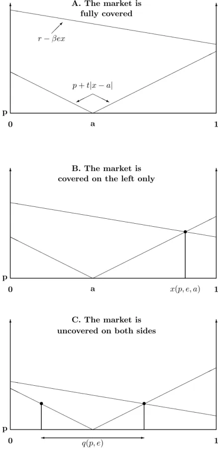
(10) location x (to the right of 12 ) verifies: r − βE = r − βex = p + t |x − a| .. (2). This is the case when r − βe − t(1 − a) ≤ p < r − a(t + 2βe). The solution of (2) is then given by x (p, e, a) ≡. r − p + ta . βe + t. (3). In such a case, the potential but unserved consumers are located on the right hand side of the market only. For p = r − a(t + 2βe), equation (2) has a lower and an upper root, respectively 0 and q(p, e) ≡ 2. r−p . 2βe + t. (4). For higher levels of p, that if r − a(t + 2βe) < p ≤ r, the market coverage is given by q(p, e) and unserved consumers can now be found on both sides of the market. In that case, the market coverage is symmetric with respect to the product variant a: it extends from a − q(p, e)/2 to a + q(p, e)/2 and thus the level of sales no longer depends on a (See Figure 1). It follows that the demand function is given by ⎧ 1 if 0 ≤ p ≤ r − βe − t(1 − a), ⎪ ⎪ ⎨ x (p, e, a) if r − βe − t(1 − a) ≤ p ≤ r − a(t + 2βe), D (p, e, a) = q(p, e) if r − a(t + 2βe) ≤ p ≤ r, ⎪ ⎪ ⎩ 0 if r ≤ p.. (5). Hence,. ⎧ ⎨ 0 Dp (p, e, a) = −1/(βe + t) ⎩ −2/(2βe + t). 3. if r ≤ p or 0 ≤ p ≤ r − βe − t(1 − a), if r − βe − t(1 − a) < p < r − a(t + 2βe), if r − a(t + 2βe) < p ≤ r.. (6). The Protected Monopolist. The monopolist makes three decisions: the product characteristics or variant a, the pollution intensity e, and the price p. We assume that those decisions are made in a two stage set-up: first the product variant a and pollution intensity e are chosen simultaneously in stage 1 and 7.

(11) then the price p in stage 2. There are many justifications for such a modeling strategy. The product characteristics (variant) choice and the technological (pollution intensity) choice are long term decisions involving important sunk costs once incurred. Price on the other hand may be considered as quite flexible. In a perfect information context with no uncertainty (our case), all decisions would be made simultaneously since there is no development of any kind between the different stages and moreover, decisions once taken will not be revised. In such a world, flexibility has literally no (real options) value and irreversibility has no cost. Considering sequential decisions is tantamount to imposing a sequence of decisions under certainty to mimic the sequence of decisions under uncertainty or imperfect information when information on market evolution or changes is gathered over time.9 The price will be determined as a function of product variant a and pollution intensity e. Given the pricing decision function, the choice of a and e can be characterized.. 3.1. The pricing decision. Let π(p, e, a) denote the profit for the monopolist: π(p, e, a) ≡ (p − c(e))D(p, e, a).. (7). From (5), the profit function is continuous in p. Moreover: Lemma 1 Given a and e, the profit function π(p, e, a) is strictly concave in p and piecewise differentiable. ¢ ¢ ¡ ¡ Proof: Let πp− p0 , e, a and πp+ p0 , e, a ) be the left-hand and right-hand partial derivatives of. the profit function with respect to p at p = p0 . From the demand function given in (5), the function π(p, e, a) is strictly concave in p on each interval where it is differentiable. Thus, it remains 9 Consider the following framework. Demand (in our case the value of r) is uncertain. The firm observes signals as time goes by which reduces the uncertainty about r. Since the decisions on product variant and technology take time (it takes time to determine the proper characteristics of the product and to install the chosen technology, that is, product variant and production/pollution technology are somewhat irreversible), the firm must decide on product variant and pollution intensity when it is relatively uninformed about r. Later, the firm observes a signal on r, so that when it makes its decision on price, it is better informed if not perfectly so. The analysis of such a context is done in our companion paper Boyer, Mahenc and Moreaux (2004).. 8.

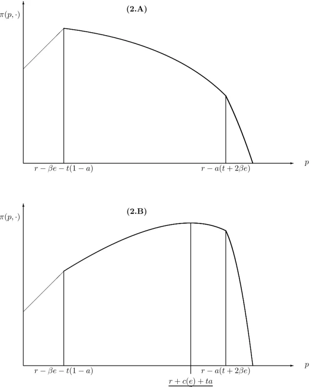
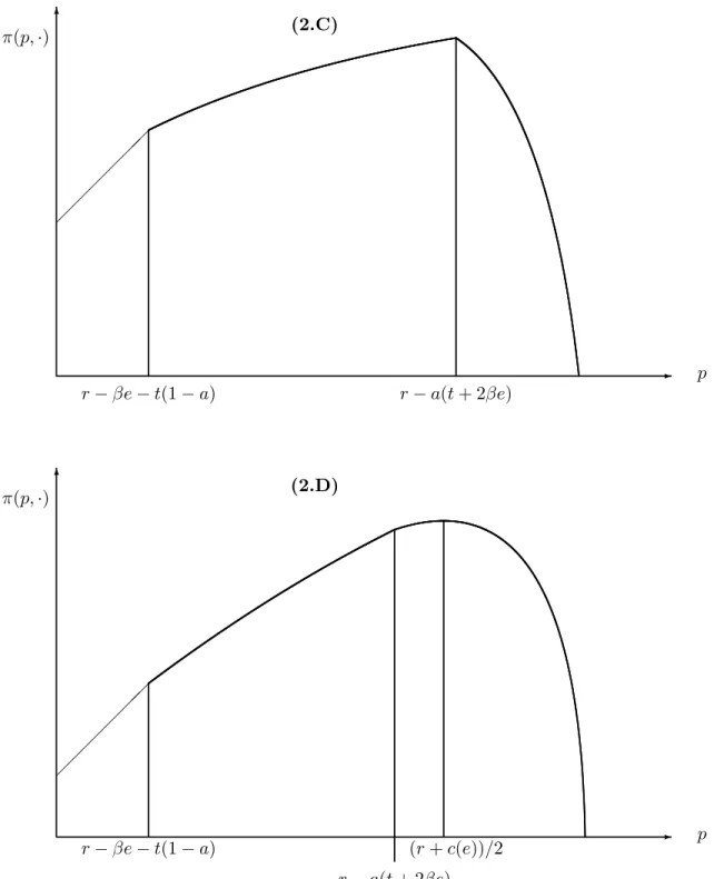
(12) to show that the function π(p, e, a) is strictly concave in the neighborhood of each point where it is not differentiable. Clearly, π(p, e, a) is strictly increasing in the interval [0, r − βe − t(1 − a)] and πp− (r − βe − t(1 − a), ·) = 1. The derivative of π(p, e, a) is πp (p, e, a) = D(p, e, a) + (p − c(e))Dp (p, e, a), where Dp (p, e, a) is given by (6). First, πp+ (r − βe − t(1 − a), e, a) < 1 since, for all p ∈ ( r − βe − t(1 − a), r − a(t + 2βe)), D (p, e, a) < 1 and Dp (p, e, a) < 0. Hence, π(p, e, a) is strictly concave in the neighborhood of r − βe − t(1 − a).. Second, from (6),. πp− (r − a(t + 2βe), e, a) > πp+ (r − a(t + 2βe), e, a). Hence π(p, e, a) is strictly concave in the neighborhood of r − a(t + 2βe).. Q.E.D.. Hence there is a unique profit maximizing price for the monopolist, denoted by pb(e, a).. The different cases are depicted in Figures 2A-2D. Defining the critical location points (critical variants) a1 , a2 , a3 as follows: a1 ≡. 2βe + 2t − (r − c(e)) r − c(e) r − c(e) , a2 ≡ > 0, a3 ≡ > 0, t 3t + 4βe 2(t + 2βe). (8). we obtain the following expressions for the profit maximizing price. Proposition 1. 1. If 2βe + 2t ≤ r − c(e), that is, a1 < 0, the profit maximizing price is pb(e, a) = r − βe − t(1 − a). (9). and the market is fully covered (Figure 2A).. 2. If 2βe + 32 t ≤ r − c(e) < 2βe + 2t, that is, a1 > 0 and a3 > a2 > 12 , then: (a) for a ∈ [0, a1 ) , the profit maximizing price is pb(e, a) = (r + ta + c(e)) /2. (10). and the market is well covered on the left side (the consumer at x = 0 strictly prefers to buy) but not on the right side (Figure 2B); 9.

(13) £ ¤ (b) for a ∈ a1 , 12 , the profit maximizing price is given by (9) and the market is fully covered (Figure 2A).. 3. If 2β + te ≤ r − c(e) < 2βe + 32 t, that is, a1 > 12 , a2 < 12 , and a3 > 12 , then: (a) for a ∈ [0, a2 ) , the profit maximizing price is given by (10) and the market is well covered on the left side but not on the right side (Figure 2B); £ ¤ (b) for a ∈ a2 , 12 , the profit maximizing price is pb(e, a) = r − a(t + 2βe). (11). and the market is just barely covered on the left (the consumer at x = 0 is indifferent between buying or not)10 but not on the right side, except at a = 4. If 0 ≤ r − c(e) < 2βe + t, that is, a1 >. 1 2. 1 2. (Figure 2C).11. and a2 < a3 < 12 , then:. (a) for a ∈ [0, a2 ) , the profit maximizing price is given by (10) and the market is well covered on the left side but not on the right side (Figure 2B); (b) for a ∈ [a2 , a3 ), the profit maximizing price is given by (11) and the market just barely covered on the left side but not on the right side (Figure 2C); ¤ £ (c) for a ∈ a3 , 12 , the profit maximizing price is pb(e, a) = (r + c(e)) /2. (12). and the market is covered neither on the left side nor on the right side (Figure 2D).. Note that in (9) and (11), the price is independent of the marginal cost c(e) while in (10) and (12), the price is independent of the marginal consumption-specific damage β. 10 The consumer at x = 0 is indifferent because, for pˆ(e, a) = r − a(t + 2βe) and x(p, a, e) given by (3), we have pˆ(e, a) + ta = r − βex. 11 The consumer at x = 1 buys the good when a = 12 because, for pˆ(e, 12 ) = r − 12 t − βe, we have r − βe = pˆ(e, 12 ) + 12 t.. 10.

(14) From the above, we can derive the effects (partial derivatives) on price pb of pollution intensity. e, product variant a, consumption-specific damage β, and preference heterogeneity factor t; they are summarized in the following proposition. Proposition 2 The monopolist’s price pb(e, a) is: • a decreasing function of e in all cases; • a non-monotonic function of a: the price is increasing in a when either the market is fully covered (expression (9)) or covered on the left but not on the right (expression (10)), decreasing in a when the market is just barely covered on the left side but not on the right side (expression (11)), and independent of a when the market is covered neither on the left side nor on the right side (expression (12)); • non-increasing with respect to consumption-specific damage β (corresponding to the partial derivative ∂ pb , hence for given e and a): the monopolist’s price decreases with β when ∂β either the market is fully covered or the market is just barely covered on the left side and not on the right side (expression (9) and (11)); otherwise the price is independent of β (expression (10) and (12)). • a non-monotonic function of t (corresponding to the partial derivative ∂ pb, hence for given ∂t e and a): the price is decreasing in t when either the market is fully covered (expression (9)) or just barely covered on the left but not on the right (expression (11)), increasing in t when the market is well covered on the left side but not on the right side (expression (10)), and the price is independent of t when the market is covered neither on the left side nor on the right side (expression (12));. When pollution intensity is lower (larger unit pollution abatement), there are two forces that complement one another to yield a price increase: first, as consumers are more willing to 11.

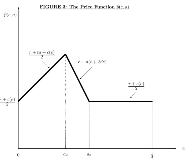
(15) pay for the product, the monopolist can extract more surplus from them, and second, marginal production costs are higher. Proposition 1 shows that the reasons why the monopolist’s price pb(e, a) is decreasing in e differ in a subtle way according to whether the whole market is covered. or not. When the whole market is covered (cases 1 and 2b in Proposition 1), the price is given by ∂ pb(e, a) (9) with = −β and therefore the monopolist increases her price to extract the additional ∂e consumer’s surplus generated by the reduction in pollution. On the other hand, when the market. is uncovered at least on one side (cases 2a, 3a, 4a and 4c in Proposition 1), the price is given by ∂ pb(e, a) (10) or (12) with = 12 c0 (e) and therefore the monopolist raises her price as a reaction ∂e to the increase in marginal production costs. Two conflicting forces explain the non monotonicity of the price as the variant a moves toward the market center. One deals with the ‘preference gap’ cost, the other with the gain of market coverage (assuming it is not complete) as price decreases. The monopolist can set a higher price (hence capture a larger part of the surplus) if the ‘preference gap’ cost decreases and the ‘preference gap’ cost decreases as a moves toward the market center. Such is the first force favoring a positive relationship between the price and the product variant as the latter moves toward the market center.12 When the market is just barely covered on the left side and not covered on the right side (cases 3b and 4b in proposition 1), then the monopolist finds it profitable to lower her price as a moves to the right in order to keep selling to the consumers on the left and gaining more consumers on the right. When a reaches a3 , then the two forces balance each other and the monopolist keeps her price constant for product variants a > a3 (case 4c of proposition 1). The price function is illustrated in Figure 3. When the market is fully covered, the lower the consumption-specific damage factor β, the higher the price charged by the monopolist since there is a larger consumer’s surplus to be captured. The monopolist captures the whole surplus of end-point consumers (x = 0 and x = 1) when a = 12 . Interestingly enough, the price remains unchanged for variations in the 12. The rate at which pˆ(e, a) increases may be t (cases 1 and 2b of proposition 1) or proposition 1).. 12. 1 t 2. (cases 2b, 3a and 4a of.

(16) consumption-specific damage factor β when the market is uncovered on both sides. In this case, p the price elasticity of demand is, from (4) and (6), given by r − p and does not directly depend on β (price p is considered as given). A larger β shifts demand downward in such a way that. for each given price, the price elasticity remains the same. Consequently, the monopolist does no longer take into account the consumption-specific damage when choosing her price. For the same reason, the consumers’ preference heterogeneity parameter t has no influence on the monopolist’s price when the market is uncovered on both sides. On the other hand, when the market is fully covered, the monopolist’s price decreases as t increases. The reason is that there is less consumers’ surplus to extract when preferences are more heterogeneous.. 3.2. Simultaneous choice of the product variant and the pollution intensity. As we mentioned before,the product characteristics (location) and the technology characteristics (pollution intensity) are both relatively inflexible once chosen and are therefore considered here as long run variables. They are chosen in a first stage followed in the second stage by the pricing decision characterized above. 3.2.1. The choice of product variant. Recognizing that whatever the values of a and e chosen, the price p will be chosen to maximize profit, the profit function can now be written in reduced form as π b(a, e) ≡ π(a, e, pb(a, e)). From Proposition 1, we obtain that the reduced-form profit function for stage 1, namely π b(a, e),. can take four different forms, where a1 , a2 and a3 are given by (8).. 1. π b(a, e) = r − βe − t(1 − a) − c(e) when either 2βe + 2t ≤ r − c(e). £ or {2βe + 32 t ≤ r − c(e) < 2βe + 2t and a ∈ a1 , 13. 1 2. ¤ };.

(17) 2. π b(a, e) = [(r + ta + c(e))/2 − c(e)]D((r + ta + c(e))/2, e, a) when. either {2βe + 32 t ≤ r − c(e) < 2βe + 2t and a ∈ [0, a1 )},. or {0 ≤ r − c(e) < 2βe + 32 t and a ∈ [0, a2 )} 3. π b(a, e) = [r − a(t + 2βe) − c(e)]q(r − a(t + 2βe), e) when. £ either {2βe + t ≤ r − c(e) < 2βe + 32 t and a ∈ a2 ,. or {0 ≤ r − c(e) < 2βe + t and a ∈ [a2 , a3 )};. 1 2. ¢. }. 4. π b(a, e) = [(r + c(e))/2 − c(e)]q((r + c(e))/2, e) = [(r − c(e))/2]q((r + c(e))/2, e) when £ ¢ {0 ≤ r − c(e) < 2βe + t and a ∈ a3 , 12 }. To characterize the optimal variant b a, we can perform a case-by-case analysis, following. Proposition 1. In what follows, the value of e is considered as given while p is given by pb(a, e). We will argue that b a = 12 .. 1. If 2βe + 2t ≤ r − c(e), then π b(a, e) = r − βe − t(1 − a) − c(e). Hence the monopolist is better off choosing b a=. 1 2. for all e.. 2. If 2βe+ 32 t ≤ r − c(e) < 2βe + 2t, then the monopolist strictly prefers b a=. 1 2. also. Indeed:. b(a, e) = (b p(e, a) − c(e))x(b p(e, a), e, a) strictly increasing in (a) For a ∈ [0, a1 ) , we have π a from (3).. £ ¤ (b) For a ∈ a1 , 12 , the market is fully covered and π b(a, e) = r − βe − t(1 − a) − c(e) is strictly increasing in a.. 3. If 2βe + t ≤ r − c(e) < 2βe+ 32 t, the monopolist is indifferent between all product variants in [a2 , 12 ]. Indeed: b(a, e) strictly increasing in a for the same reason as in case (a) For a ∈ [0, a2 ) , we have π 2a above.. 14.

(18) £ ¤ (b) For a ∈ a2 , 12 , the profit π b(a, e) is given by (b p(e, a) − c(e))x(b p(e, a), e) is strictly increasing in a.. 4. If 0 ≤ r − c(e) < 2βe + t, then, whatever e, we have π b(a, e) strictly increasing in a for £ ¤ a ∈ [0, a2 ), increasing in a for a ∈ a2 , 12 , and constant for variants in [a3 , 12 ]. To determine a unique profit maximizing product variant for the monopolist, we must introduce either a variant cost or a refinement concept to identify the most likely product variant among all those which maximize profit. Introducing a variant cost in the space of characteristics may be somewhat arbitrary unless we can derive it from empirical observations which can only be specific to the industry or product class considered.13 In the context we have considered so far in this paper, the preferred route is clearly to introduce a refinement concept. It is reasonable to assume that when the monopolist is indifferent between a set of product variants, she chooses the one which maximizes global consumer surplus, that is the surplus of all consumers, actual and potential. Given that the ‘preference gap’ cost is linear, this means that the monopolist will choose a product variant as close as possible to 12 , the center of the market. Hence, Proposition 3. The monopolist always chooses a product variant at the market center. The monopolist always choose the product variant that is the most appealing to consumers, that is, the variant which maximizes the interest of potential consumers in the product. In other words, she chooses the variant which minimizes the total ‘preference gap’ cost over all potential consumers. 13. One could claim that given that a = is more expensive to design.. 1 2. is appealing to more people, it would be reasonable to expect that it. 15.

(19) 3.2.2. The choice of the pollution intensity. Maximizing her profit given a and e,the monopolist chooses the price pb(e, a) such that πp (b p(e, a), e, a) = 0.14 It follows that. p(e, a), e, a). D(b p(e, a), e, a) = −(b p(e, a) − c(e))Dp (b. (13). Now the variant b a = 1/2 is chosen independently of the pollution intensity e and we can characterize the monopolist’s choice of e as maximizing the reduced-form profit function π b(e, 1/2) ≡ (b p(e, 1/2) − c(e))D(b p(e, 1/2), e, 1/2). with respect to e. The following analysis shows that the profit function π b(e, 1/2) attains a unique maximum which is denoted by eb.. From the analysis leading to Proposition 2, we know that the monopolist will, conditional. on e, either covers the whole market or leaves some consumers unserved on both sides of the market.15 From proposition 1, we know that the market will be fully covered when the monopolist chooses b a=. 1 2. and pollution intensity e in the closed interval © ª EM ≡ e ∈ R+ | r − c(e) − t − 2βe ≥ 0 ,. while choosing the profit maximizing price pb(e, 1/2) in stage 2. Let e1 and e2 be respectively. the left endpoint and the right endpoint of EM ,16 that is, the minimal and maximal pollution intensities for which the market is fully covered. For matter of simplicity and to concentrate on the more interesting cases, we will make four specific assumptions, which could clearly be relaxed at the cost of a more lengthy and complex analytical treatment. The first assumption says that the production costs under no pollution would be high enough that the monopolist would not cover the whole market: 14. The profit function π(ˆ p(e, a), e, a) is not always differentiable with respect to p at its maximum. At such point, the left derivative is positive and the right derivative is negative. 15 When a = 12 , both sides of the market are symmetric. 16 The set EM expands with reservation value r and shrinks with the preference-gap cost factor t and with the marginal consumption-specific damage β.. 16.

(20) Assumption 1: r − c(0) − t < 0. It follows from Proposition 1(4c) that pb(0, 1/2) = (r + c(0)) /2. We will also assume that the monopolist’s profit increases with e for e ≤ e1 , namely:. Assumption 2: πe (e, 1/2) > 0 for all e ≤ e1 . Hence, the profit maximizing pollution intensity will either be in EM or to the right of e2 . To concentrate on the more interesting and relevant cases, we will assume that for β = 0 (no consumption-specific damage or no environmentally aware consumers), the monopolist, choosing the pollution intensity e at which c0 (e) = 0, would not cover the whole market (while charging a price pb(e, 1/2) given by (12)), namely: Assumption 3: e2 < e.. Finally, as a sufficient condition for the second-order conditions to be satisfied (below), we will assume that the cost function is sufficiently convex in the following sense: Assumption 4: For all e, c0 (e)2 < (r − c(e))c00 (e). We first consider the maximization of π b(e, 1/2) in EM . For all e inside EM , the market is. fully covered and therefore the reduced-form profit function is π b(e, 1/2) = r − βe − t/2 − c(e),. which is concave in e due to the convexity of c(e). Hence, the function attains a unique local maximum in EM , which we shall denote by ee. If ee is in the interior of EM , then π be (˜ e, 1/2) = −β − c0 (˜ e) = 0.. (14). Let us now consider the maximization of π b(e, 1/2) outside EM . The market is then covered. neither on the left side nor on the right side. Given b a = 1/2, the monopolist’s profit is π b(e, 1/2) = (b p(e, 1/2) − c(e))q(b p(e, 1/2), e). where pb(e, 1/2) = (r + c(e)) /2 (case 4c of Proposition 1). We get. p(e, 1/2) − c(e))qe (b p(e, 1/2), e) − q(b p(e, 1/2), e)c0 (e) π be (e, 1/2) = (b +πp (b p(e, 1/2), e, 1/2)b pe (e, 1/2). 17. (15).

(21) From the envelope theorem, the indirect effect of e on π b(e, 1/2) through the change in price. is zero since the optimal price pb(e, 1/2) satisfies πp (b p(e, 1/2), e, 1/2) = 0. But there is a conflict. between the two effects captured by the first two terms of (15). The first term is a demand. effect: From (4), increasing the pollution intensity level shifts demand downward and reduces profit. The second term is a cost effect: Increasing the pollution intensity level reduces the production cost and increases profit. Substituting D(b p(e, b a), e, a) = q(b p(e, 1/2), e) in (13), we ³ ´ obtain: pb(e, 1/2) − c(e) = − q(·)/qp (·) . The derivative π be (e, 1/2) can then be written as, using pb for pb(e, 1/2) when no confusion is possible:. µ ¶ p, e) qe (b π be (e, 1/2) = q(b − c0 (e) . p, e) − qp (b p, e). (16). Using (4) and (6), we obtain:. ¡ ¢ π be (e, 1/2) = q(b p, e) −βq(b p, e) − c0 (e) .. (17). Hence, the first order condition for profit maximization outside EM yields −βq(b p, e) − c0 (e) = 0, (from which, eb < e) and the second order condition requires. p, e)qe (b p, e) − qe (b p, e)c0 (e) − q(b p, e)c00 (e) < 0. π bee (e, 1/2) = −2βq(b. (18). (19). The monopolist’s production level as a function of e is given by q(e) ≡ q(b p(e, 1/2), e) = q. µ. ¶ r − c(e) r + c(e) ,e = . 2 2βe + t. (20). Hence, qe (b p(e, 1/2), e) =. −c0 (e) − 2βq(e) ; 2βe + t. (21). substituting the first-order condition (18) into equation (21) yields dq((b p(e, 1/2), e) ¯¯ βq(b e) < 0. = qe (b e) = − ¯ de 2βb e+t e=ˆ e 18. (22).

(22) Condition (22) holds for e = eb but not in general.. Using (20) and (21), the second order condition given by (19) is equivalent to (2βq(b p, e) + c0 (e))2 − (r − c(e))c00 (e) < 0,. (23). which is satisfied under Assumption 4. Furthermore, we have π be− (e2 , 1/2) = −β − c0 (e2 ) =. π be+ (e2 , 1/2) from (17), which means that the profit function is differentiable at e2 . Hence, under. Assumptions 1 to 4, (14) and (18), one of the following two cases appears at the right endpoint e2 of EM :. b(e, 1/2) is maximized at ee in EM and therefore 1. either we have −c0 (e2 ) ≤ β, in which case π eb = ee and −c0 (b e) = β;. 2. or we have −c0 (e2 ) > β and π b(e, 1/2) is maximized at eb above e2 (but below e), where, from (18), −c0 (b e) = βq(b p, eb).. Proposition 4A.. The profit maximizing intensity of pollution eb chosen by the monopolist satisfies e). βD(b p, eb, 1/2) = −c0 (b. (24). The monopolist chooses a level of pollution intensity e that is lower than the level a competitive producer would choose. The monopolist chooses to generate a level of pollution at which the marginal benefit of pollution in terms of a reduced production cost, −c0 (b e), equals the marginal consumption-specific damage from pollution incurred by all served consumers, βD(b p, eb, 1/2). This strongly contrasts. with the behavior of a price-taking competitive producer who would generate a level of pollution ec = e at which the marginal benefit of pollution in terms of a reduced production cost c0 (ec ) is zero. Unlike the competitive producer, the monopolist takes into account the consumers’ willingness to pay for a clean and/or safe environment. She recognizes the effect of pollution on the 19.

(23) NWP and of the NWP on her profit maximizing price, to the extent that the detrimental effect of pollution has a consumption-specific component. The monopolist internalizes the externality, at least in part, because she behaves strategically with respect to consumers and properly takes into account their reaction to changes both in the pollution intensity level and the price level. Proposition 4B.. • If −c0 (e2 ) ≤ β, then D(b p, eb, 1/2) = 1.. • If −c0 (e2 ) > β, then D(b p, eb, 1/2) = q(b p(b e, 1/2), eb) < 1.. An interpretation of condition −c0 (e2 ) ≤ β is that the marginal benefit of pollution (in reducing production costs) is lower than the marginal consumption-specific damage when the market is not fully covered, since −c0 (e) < −c0 (e2 ) for all e ∈ [e2 , e). In this case, the monopolist is better off reducing pollution intensity until the whole market is covered: the consumers’ relatively large willingness to pay to reduce pollution is large enough to dominate the negative impact of the increase in production costs. On the other hand, when −c0 (e2 ) > β, the marginal consumptionspecific damage β is smaller than the marginal benefit of pollution −c0 (e) when e < e2 , that is, when the market is fully covered. In this case, the monopolist is better off increasing pollution intensity above e2 even though she losses some consumers (among the more reluctant to buy her product). When the market is fully covered (production or market coverage is constant at 1) for e = eb, the intensity of pollution eb also represents the monopolist’s total pollution which thus. increases with eb. When the market is not fully covered, the monopolist’s overall level of pollution. E(b e) = ebq(b p, eb) increases with pollution intensity eb since, using (22), Ee (b e) = q(b p, eb) + ebqe (b p, eb) =. t + βb e q(b p, eb) > 0. 2βb e+t 20. (25).

(24) As previously seen, the total derivative qe (b p, e) evaluated at e = eb is negative, showing that a higher intensity of pollution eb has both a positive direct effect on total pollution, captured by. the first term in the right hand side of (25), and an indirect negative effect through the decrease. in the monopolist’s production level. The direct effect of e on total pollution dominates the indirect effect. As a result, a lower intensity of pollution in the neighborhood of eb results in. a wider market coverage (if not already fully covered), a lower global level of pollution, and a r + c (e) higher price since pb(e, 1/2) = decreases with e in the interval [e2 , e). Hence: 2 Proposition 4C.. Evaluated at e = eb, the relation between the global level of pollution E and the pollution intensity level e is positive. Indeed,. dE ¯¯ d[eq(b p(e, 1/2), e)] ¯¯ = < 0. ¯ ¯ de e=ê de e=ˆ e. The proposition below summarizes the results for the unregulated monopolist. Proposition 5. The unregulated monopolist behaves as follows. 1. If at the right endpoint of EM , we have −c0 (e2 ) ≤ β, then the unregulated monopolist covers the whole market by choosing a product variant at the center of the Hotelling market, a pollution intensity level eb satisfying β = −c0 (b e), and a price pb(b e, 1/2) = r −βb e −t/2. Hence pbe (b e, 1/2) < 0 and production is constant at 1, in which case the global level of pollution. E(b e) is equal to eb.. 2. If at the right endpoint of EM , we have −c0 (e2 ) > β, then the unregulated monopolist leaves consumers unserved on both sides of the market by choosing a product variant at the center of the market, a pollution intensity level eb < e satisfying βq(b p(b e, 1/2), eb) = −c0 (b e), where 0 r + c (b e) c (b r − c (b e) e) e, 1/2) = . Hence, pbe (b = − β , and a price pb(b e, 1/2) < q(b p(b e, 1/2), eb) = 2 t + 2βb e 21.

(25) 0 and qbe (b p(b e, 1/2), eb, 1/2) < 0; moreover, the global level of pollution E(e) = eq(b p(e, 1/2), e) is increasing in e at e = eb.. The monopolist’s price always decreases in e, albeit for different reasons according to whether the monopolist fully covers the market or not. First, when the monopolist covers the whole market, a reduction in pollution intensity induces her to capture an additional surplus from consumers since they are willing to pay more for a cleaner product. Thus, the monopolist raises her price. Second, when the monopolist finds it more profitable not to cover the whole market, the reduction in pollution intensity, raising marginal production costs, induces the monopolist to raise also her price and, interestingly enough, to produce more. As mentioned by an anonymous referee, the present result that the monopolist raises her price as pollution intensity decreases, is not specific to the horizontal differentiation in consumers’ taste. This result may be true, for instance, in the following vertical differentiation context which is reminiscent of Mussa and Rosen (1978) or Gabszewicz and Thisse (1979):17 consumers have heterogeneous reservation values for the product given by r/e, where r is uniformly distributed over [0, R]; they derive a surplus r/e − p from purchasing the good at price p; hence, the demand function is given by 1 − ep/R. Moreover, the interested reader can check that the result that the monopolist’s price declines with pollution intensity also holds with structures of the demand function that are more general than the linear ones, to the extent that demand decreases with e.. 3.3. The impact of the consumption-specific damage factor β.. Given the parameters of the problem at hand, the monopolist’s choices of product characteristics, pollution intensity and price are the result of three forces: market power, the positive benefit of pollution intensity in terms of cost reduction, and the negative impact of pollution on the consumers’ willingness to pay for the product. To measure the impact of the consumption17. We are grateful to Philippe Bontems for suggesting this example.. 22.

(26) specific damage factor β on the monopolist’s choice of pollution intensity and price, let us define β e the following elasticity η of pollution intensity with respect to β: η ≡ db . We show below that eb dβ this elasticity is negative regardless of the market coverage. Thus, the higher the consumptionspecific damage (or the more environmentally aware consumers are), the lower the pollution intensity chosen by the unregulated monopolist. Moreover, we will show that the absolute value of η determines whether the consumption-specific damage has a positive or a negative effect on db p the monopolist’s price, that is, whether dβ is positive or negative. Using Proposition 5, we obtain Proposition 6.. • The pollution intensity level eb decreases with β.. • If −c0 (e2 ) ≤ β, the market is fully covered and the monopolist’s price increases with β if η < −1 while it decreases with β if η > −1. • If −c0 (e2 ) > β, the market is partially covered and the monopolist’s price increases with β while the production level increases with β if η < −2 while it decreases with β if η > −2. Proof: As long as the market is fully covered, then from (9), we have db p(b e, 1/2) db e = −b e−β = −b e(1 + η). dβ dβ Taking then the total differential of (14) yields db πe (b e, 1/2) = −dβ − c00 (b e)db e = 0, that is 1 db e = − 00 < 0; dβ c (b e). (26). hence the elasticity η is negative and the first part of the proposition follows if the market is fully covered. On the other hand, when some consumers on both sides are unserved, then, from (12), we have db p(b e, 1/2) 1 1 eb eb = c0 (b = c0 (b e) e) η, dβ 2 dβ 2 β 23.

(27) whose sign depends on η. To obtain the expression for η in this case, let us substitute q(b p, e) r − c(e) from (20) in equation (24), which yields β + c0 (e) = 0, and take the total differential to 2βe + t obtain db e e) r − c(b e) + 2b ec0 (b =− 0 . 00 dβ βc (b e) + c (b e)(t + 2βb e) From (20), we get that q(b p(b e, 1/2), eb) = −. c0 (b e) . Using this equation yields β. tq(b p(b e, 1/2), eb)2 db e = 0 2 < 0 by Assumption 4; dβ c (b e) − (r − c(b e))c00 (b e). hence η < 0 and. db p(b e, 1/2) > 0. Moreover, from (20) and (22), we obtain dβ dq(b p, eb) dβ. = −2b e. =. r − c(b e) e βq(b e) db 2 − 2βb e + t dβ (2βb e + t). ebq(b e) (−2 − η) ; 2βb e+t. hence the remainder of the proposition follows. Q.E.D.. Increases in the consumption-specific damage factor β generates two conflicting effects on the monopolist’s price. The direct effect is that the monopolist charges a lower price as there is less surplus to extract from consumers. The indirect effect is that the monopolist chooses a lower level for pollution intensity, which increases both consumers’ surplus and production costs. The increase in consumers’ surplus in turn relaxes the downward pressure on price. Consider first that the market is fully covered. The indirect effect dominates the direct effect on price provided that η is larger than one in absolute value (b e is β-elastic): the monopolist raises her price as consumption-specific damage increases. By contrast, when η is less than one in absolute value (b e is β-inelastic), the monopolist reduces her price as consumption-specific damage increases. Consider now the case where the market is uncovered on both sides. As previously seen, the price elasticity of demand does not depend on β. Consequently, the direct effect on price 24.

(28) of an increase in β vanishes and the indirect effect is the only active one. Thus, confronted with an increase in β, the monopolist reduces pollution intensity, raises her price because she incurs higher production costs, and at the same time increases production and market coverage provided that eb is sufficiently β-elastic, namely η is larger than two in absolute value.. 4. The regulated choice of the pollution intensity. Suppose that a regulator can determine the emission intensity level e, leaving the choice of a and p(a, e) to the monopolist. This is a second-best problem which concentrates on the efficiency of the pollution abatement control as the sole mean of command. Environmental regulation is done in most countries through a separate regulatory authority, which operates more or less independently from other regulatory authorities, such as those dealing with antitrust, competition policy, copyrights and patents, or occupational health and safety standards. In order to see the specific effects of a stand alone environmental regulatory authority in the present context, we assume that none of the other regulatory controls are present and that the environmental regulator’s sole instrument is indeed the pollution intensity parameter e. Note however that, in the present context, it amounts to a complete control on the production technology.18 The choice of e is made in stage one by the regulator while a in stage one and p in stage two remain under the control of the monopolist. Let e∗ denote the pollution intensity standard chosen by the regulator. From Proposition 3, we know that the monopolist chooses a product variant at the market center regardless of e: b a(e∗ ) = 1/2. The social welfare is defined as the sum of consumers’ and monopolist’s surplus less environmental damages. Given a price p, the. profit is p − c(e) per consumer or per unit consumed and the net surplus of a consumer located 18. Alternatively, the regulatory control could be modeled as affecting directly the characteristics of the product, hence the choise of location a in the present case. In some applied cases, it is not the technology but the product characteristics that are controlled by the regulator. Indeed, our preliminary results, not reproted here, show that the regulator may choose a location a∗ away from the market center in order to make the product either less accessible or less desirable for some consumers, namely those located closer to one of the end points of the market line. See Boyer, Mahenc, Moreaux (2004) for more on this regulatory policy for environmental protection.. 25.

(29) at x is given by r − (1 + β) d(E) − t |x − 1/2| − p if he purchases the good at price p from the monopolist located at the market center, and −d(E) otherwise. The regulator’s objective is to maximize the sum of profit and net consumer surplus over all those consuming the product, that is, r − βd(E) − t |x − 1/2| − c(e), less the global damage from pollution d(E), which affects both served and unserved consumers. Suppose the level of production is q and let A(q, e) denote the set of consumers (consumer locations) with a positive surplus given the product variant b a = 1/2 and that level of output q: A(q, e) ≡ {x ∈ [0, 1] : r − βeq − t |x − 1/2| − c(e) ≥ 0} .. The social welfare function W (q, e) can then be written as follows: Z [r − βeq − t |x − 1/2| − c(e)] dx − eq W (q, e) = A(q,e). = (r − c(e) − βeq − e)q − tq 2 /4. (27). Given a pollution intensity standard e, the monopolist located at the market center chooses in stage 2 the price pb(e, 1/2) characterized in Proposition 1. When choosing e, the regulator. anticipates that the monopolist will charge pb(e, 1/2) and produce up to a level that satisfies the demand expressed at that price. From (5), we get: ⎧ ⎨ 1, D(b p(e, 1/2), e, 1/2) = ⎩ q(b p(e, 1/2), e). if 2βe + t ≤ r − c(e),. (28). if 0 ≤ r − c(e) ≤ t + 2βe.. Social welfare W (D(b p(e, 1/2), e, 1/2), e) can thus be written as. Z. A(D(ˆ p(e,1/2),e,1/2),e). [r − βeD(b p(e, 1/2), e, 1/2) − t |x − 1/2| − c(e)] dx − eD(b p(e, 1/2), e, 1/2). From now on, we will use the simplified notations: W (e). ≡. W (D(b p(e, 1/2), e, 1/2), e),. π(e). ≡. q(e). ≡. π b(1/2, e) = (b p(e, 1/2) − c(e)) D(b p(e, 1/2), e, 1/2),. r − c(e) q(b p(e, 1/2), e) = t + 2βe . 26.

(30) Hence the following expressions for social welfare: ⎧ r − c(e) − (1 + β)e − t/4 = π(e) + t/4 − e, ⎪ ⎪ ⎪ ⎪ if t + 2βe ≤ r − c(e) ⎪ ⎪ ⎪ ⎪ (the market is fully covered); ⎨ W (e) = ⎪ ⎪ (r − c(e) − βeq(e) − e)q(e) − tq(e)2 /4 = π(e) + tq(e)2 /4 − eq(e), ⎪ ⎪ ⎪ ⎪ ⎪ if 0 ≤ r − c(e) ≤ t + 2βe ⎪ ⎩ (the market is uncovered on both sides).. (29). Clearly, the private and the social incentive to curb pollution emissions have no reason to coincide. The environmental regulator is responsible for achieving an optimal balance between the cost of abatement (the monopolist’s benefit of pollution) and the global damage from pollution, while it is only the consumption-specific damage that is of concern to the unregulated monopolist. The derivative We is given by: ⎧ ⎨ πe (e) − 1, We (e) = ⎩ πe (e) + tq(e)qe (e)/2 − q(e) − eqe (e),. if t + 2βe ≤ r − c(e);. (30). if 0 ≤ r − c(e) ≤ t + 2βe.. Moreover, using Proposition 4, the derivative of welfare W with respect to the pollution intensity e, evaluated at the pollution intensity chosen by the monopolist eb, is: ⎧ if t + 2βb e ≤ r − c(b e); ⎪ ⎨ −1, e) = We (b ⎪ e) ⎩ − q(b (βb e + t + βtq(b e)/2) < 0, if 0 ≤ r − c(e) ≤ t + 2βe. t + 2βb e. (31). A straightforward consequence of (31) is that the welfare maximizing pollution intensity level satisfies: e∗ < eb. To determine whether this local maximum is a global maximum, we must study. the behavior of We (e) in the neighborhood of e1 and e2 . For matter of simplicity, let us assume that W (e) is increasing in [0, e1 ], so that the optimum is above e1 ; this allows us to concentrate on e2 . From (31), we have We− (e2 ) = πe− (e2 ) − 1 and We+ (e2 ) = πe+ (e2 ) − 1 + qe (e2 ) (t/2 − e2 ). Remembering that π be− (e2 , 1/2) = π be+ (e2 , 1/2), we obtain that the welfare function W (e) is not. differentiable at e2 and may be concave or not, depending on the sign of qe (e2 ) (t/2 − e2 ). A. sufficient condition for W (e) to be concave at e2 is that the left hand derivative be larger than 27.

(31) or equal to the right hand derivative or, equivalently, that qe (e2 ) (t/2 − e2 ) ≤ 0 where qe (·) is given by (21). We will make the following assumption: Assumption 5: We− (e2 ) ≥ We+ (e2 ) Assumption 5 is verified when, either −c0 (e2 )/2 ≤ β and t/2 ≥ e2 , that is, consumers’ preferences are sufficiently heterogeneous (t large) when the consumption-specific damage they incur is rather high, or −c0 (e2 )/2 ≥ β and t/2 ≤ e2 , that is, consumers’ preferences are sufficiently homogeneous (t low) when the consumption-specific damage they incur is rather low. We can now compare the market coverages of both monopolists, regulated and unregulated. This is done in the next proposition. Under assumption 5, three cases must be considered depending on how significant is the marginal benefit of pollution at e2 , that is −c0 (e2 ), relative to the marginal damages, both consumption-specific and global. Proposition 7. Under assumption 5,. 1. if −c0 (e2 ) < β, then e∗ < eb < e2 and q(b e) = q(e∗ ) = 1,. 2. if β ≤ −c0 (e2 ) ≤ 1 + β then e∗ < e2 < eb and q(b e) < q(e∗ ) = 1,. 3. if 1 + β < −c0 (e2 ) then e2 < e∗ < eb and q(b e) < q(e∗ ) < 1.. In case 1, the marginal benefit of pollution is lower than the marginal consumption-specific damage when the market is not fully covered. The unregulated monopolist is better off choosing eb < e2 and so covers the whole market. From (31), We− (e2 ) < 0 and assumption 5 is sufficient to. ensure the concavity of W (e). Assumption 5 is equivalent here to t/2 ≥ e2 since qe (e2 ) ≤ 0, that. is, consumers’ preferences must be sufficiently heterogeneous. In this case, the regulator chooses a pollution intensity standard e∗ < eb such that 1 + β = −c0 (e∗ ). This is the Samuelson condition for the optimal provision of the public bad: the efficient standard of pollution intensity requires. that the monopolist’s private marginal cost saving from polluting is equal to the marginal global. 28.

(32) damage, hence is equal to the sum over all consumers of their willingness to pay for reducing the pollution generated by production. Then, the market is fully covered regardless of whether the monopolist is regulated or not. In case 2, the marginal consumption-specific damage is lower than the marginal benefit of pollution when the market is fully covered, namely β ≤ −c0 (e2 ), and the marginal benefit of pollution is lower than the marginal global damage when the market is not fully covered, namely We− (e2 ) ≤ 0 or, equivalently, −c0 (e2 ) ≤ 1 + β. From Proposition 5, the unregulated monopolist leaves consumers unserved on both sides of the market by choosing eb ≥ e2 . Furthermore,. assumption 5 ensures the concavity of W (e): the regulator chooses e∗ < e2 < eb and the market. is then fully covered.. In case 3, the marginal damages, both consumption-specific and global, are lower than the marginal benefit of pollution when the market is fully covered. Then the regulator chooses e∗ ∈ [e2 , eb) and the market coverage is partial if We+ (e2 ) > 0. Under the latter condition, the regulator chooses e∗ solving equation. πe (e) + tq(e)qe (e)/2 = q(e) + eqe (e) = Ee (e),. (32). which equates the marginal social value of the pollution intensity standard to the marginal global damage. Moreover, it follows from lemma 2 and Proposition 5 that more consumers are served at a higher price by the monopolist subject to environmental regulation than by the unregulated monopolist. Proposition 8.. • The unregulated monopolist pollutes more and produces as much or less than the regulated monopolist whatever the market coverage. If the efficient market coverage is partial, the unregulated monopolist produces strictly less, pollutes strictly more, and charges a lower 29.

(33) price than the monopolist subject to environmental regulation. If the unregulated monopolist was covering the whole market, she still does it when subject to environmental regulation. If she was not covering the whole market, then she increases production when subject to the regulatory pollution intensity standard.. This proposition sheds light on the social inefficiencies of a polluting monopolist confronted to environmentally aware consumers. The unregulated monopolist always pollutes too much from the environmental regulator’s viewpoint. Moreover, the unregulated monopolist would always raise her price if she were asked to reduce pollution intensity, either to benefit from the resulting increase in consumers’ surplus or as a reaction to the resulting increase in her production costs or both. By contrast, it may happen that the unregulated monopolist is better off covering the whole market when social efficiency requires to do so: such is the case when the marginal benefit from pollution is low relative to the marginal consumption-specific damage. Otherwise, according to the regulator’s benchmark, the unregulated monopolist produces too little, in which case she would actually extend the market coverage and simultaneously raise price to meet the regulator’s requirement. The main technical difficulties with the present analysis emerge from the fact that the demand function is not everywhere differentiable. By contrast, the case in which the efficient market coverage is partial — namely case 3 in Proposition 7 — turns out to be “well-behaved” in the sense that the demand function is everywhere differentiable. Then, the model has strong affinities to Spence (1975) who addresses the problem of regulating the quality choice of a monopolist. The latter is shown to undersupply quality relative to the social optimum when the consumer’s marginal valuation of quality decreases with quantity. Our result is somewhat related to Spence’s result: the unregulated monopolist pollutes more than the regulated monopolist. Interestingly enough, it can be checked from (4) that the inverse demand curve is given by P (q, e) = r − (2βe + t)q/2. Thus Pqe < 0: paraphrasing Spence, the consumer’s marginal valuation of environmental quality decreases with quantity. This provides new insight on the 30.

(34) consequence of reducing pollution intensity on the monopoly price. The first effect is that consumers are willing to pay more for the product. This upward-shift in demand induces the monopolist to extract more surplus from the consumers. The second effect is that production costs are higher, which gives the monopolist a further incentive to raise price.. 5. Conclusion. In Hotelling’s (1929) horizontal differentiation context, the emergence of consumers concerned with an individual damage due to pollution compels the monopolist to pollute less. Clearly, this is beneficial from the environmental regulator viewpoint. Depending on the β-elasticity of the pollution intensity at its optimal level, the monopolist serves fewer or more consumers while raising her price relative to what would prevail with environmentally unaware consumers. Nevertheless, the unregulated monopolist’s choice of pollution intensity is biased upward with respect to the environmental regulator’s target because the monopolist disregards the global damage and only takes into account the consumption-specific damage when maximizing profit; thus, the pollution externality fails to be fully internalized. A notable result is that the monopolist’s price declines with pollution intensity. This illustrates that the presence of environmentally aware consumers is likely to exacerbate the conflicts between an environmental regulator and an economic regulator which is responsible for controlling market power, in particular the pricing policy of a monopolist, such as a public utility commission. In the present context, if the monopolist is asked by the environmental regulator to reduce pollution intensity, then she will have two incentives to raise her price: first, a higher price allows the monopolist to extract more surplus from consumers since they are willing to pay more for a cleaner product; second, a cleaner product entails higher production costs for the monopolist, hence induces her to raise price. However, the potential increase in price clearly complicates the task of the economic regulator. However, further research will be needed to study more generally the influence of demand elasticity on pollution intensity distortion when 31.

(35) consumers are environmentally aware. Given the increasing environmental awareness among consumers and policy makers, this topic should be high on the agenda of academic researchers.. 32.

(36) References [1] BANSAL, S. and S. GANGOPADHYAY (2003), “Tax/Subsidy Policies in the Presence of Environmentally Aware Consumers”, Journal of Environmental Economics and Management 45, 333-355. [2] BARNETT, A. (1980), “The Pigouvian Tax Rule under Monopoly”, American Economic Review 70, 1037-1041. [3] BARON, D. P. (1985), “Regulation of Prices and Pollution under Incomplete Information”, Journal of Public Economics 28, 211-231. [4] BAUMOL, J. and W. E. OATES (1975), The Theory of Environmental Policy, Second Edition, Cambridge: Cambridge University Press. [5] BOYER, M. and G. DIONNE (1983), “Riscophobie et étalement a` moyenne constante : Analyse et applications,” Actualité économique / Revue d’analyse économique 59, 208-229. [6] BOYER, M., P. MAHENC and M. MOREAUX (2004), “The role of environmental awareness in environmental protection,” working paper, Université de Perpignan. [7] BUCHANAN, J. M. (1969), “External Diseconomies, Corrective Taxes and Market Structures”, American Economic Review 59, 174-177. [8] CARRARO, C., Y. KATSOULACOS and A. XEPAPADEAS eds. (1996), Environmental Policy and Market Structure, Dordrecht: Kluwer Academic Publishers. [9] CARRARO, C. and A. SOUBEYRAN (1996), “Environmental Taxation, Market Share and Profits in Oligopoly” in Carraro, C., Y. Katsoulacos and A. Xepapadeas (eds) Environmental Policy and Market Structure, Dordrecht: Kluwer Academic Publishers. [10] CASON T. N. and L. GANGADHARAN (2002), “Environmental Labelling and Incomplete Consumer Information in Laboratory Experiments”, Journal of Environmental Economics and Management 43, 113-134. 33.

(37) [11] CONRAD, K. and J. WANG (1993), “The Effect of Emission Taxes and Abatement Subsidies on Market Structure”, International Journal of Industrial Organization 11, 499-518. [12] FOULON J., P. LANOIE and B. LAPLANTE (2002), “Incentives for Pollution Control; Regulation or Information?”, Journal of Environmental Economics and Management 44, 169-187. [13] GABSZEWICZ, J. and J. F. THISSE (1979), “Price Competition, Quality and Income Disparities”, Journal of Economic Theory 20, 340-359. [14] HOTELLING H. (1929), “Stability in Competition”, Economic Journal 39, 41-57. [15] INNES R. and J. J. BIAL (2003), “Inducing Innovation in the Environmental Technology of Oligopolistic Firms”, The Journal of Industrial Economics 51, 265-287. [16] KOLSTAD, C. D. (2000), Environmental Economics, Oxford University Press. [17] LEVIN, D. (1985), “Taxation within Cournot Oligopoly”, Journal of Public Economics 27, 281-290. [18] MUSSA, M. and S. ROSEN (1978), “Monopoly and product Quality”, Journal of Economic Theory 18, 301-317. [19] SPENCE A. M. (1975), “Monopoly, Quality and Regulation”, The Bell Journal of Economics 6, 417-429. [20] TIETENBERG, T. (2000), Environmental and Natural Resource Economics (5th edition), Addison Wesley Longman.. 34.

(38) FIGURE 1: The Market Coverage. A. The market is. 6 6 hhhh hhhh fully covered hhhh hhhh µ ¡ hhhh ¡ hhhh hhhh r − βex. p. © ©© © ©© H © HH ©© © HH p + t|x − a| © HH ©© ©©HH HH© ¼ j©© H HH©©. a. 0. 1. B. The market is covered on the left only. 6. 6. hhhh hhhh hhhh hhh hhhh ©© hhhh ©© h•hhh h ©© H © © HH ©© HH © HH ©© © HH HH©©© p. a. 0. C. The market is uncovered on both sides. 6. p. x(p, e, a). 1. 6. ©© © © hhhh hhhh ©© H hhhh © HH hhhh ©© hhh © H•H • h hhhh ©© HH hhhh © © HH © HH©©. 0. ¾. -. q(p, e). 1.

(39) FIGURE 2: The Profit Function. 6. (2.A). π(p, ·) ¡ ¡ ¡ ¡ ¡ ¡. r − βe − t(1 − a). 6. -. p. -. p. r − a(t + 2βe). (2.B). π(p, ·). ¡ ¡ ¡ ¡ ¡ ¡. r − βe − t(1 − a). r − a(t + 2βe) r + c(e) + ta 2.