Série Scientifique
Scientific Series
2002s-50
Forecasting Non-Stationary
Volatility with
Hyper-Parameters
CIRANO
Le CIRANO est un organisme sans but lucratif constitué en vertu de la Loi des compagnies du Québec. Le financement de son infrastructure et de ses activités de recherche provient des cotisations de ses organisations-membres, d’une subvention d’infrastructure du ministère de la Recherche, de la Science et de la Technologie, de même que des subventions et mandats obtenus par ses équipes de recherche.
CIRANO is a private non-profit organization incorporated under the Québec Companies Act. Its infrastructure and research activities are funded through fees paid by member organizations, an infrastructure grant from the Ministère de la Recherche, de la Science et de la Technologie, and grants and research mandates obtained by its research teams.
Les organisations-partenaires / The Partner Organizations
•École des Hautes Études Commerciales •École Polytechnique de Montréal •Université Concordia
•Université de Montréal
•Université du Québec à Montréal •Université Laval
•Université McGill
•Ministère des Finances du Québec •MRST
•Alcan inc. •AXA Canada •Banque du Canada
•Banque Laurentienne du Canada •Banque Nationale du Canada •Banque Royale du Canada •Bell Canada
•Bombardier •Bourse de Montréal
•Développement des ressources humaines Canada (DRHC) •Fédération des caisses Desjardins du Québec
•Hydro-Québec •Industrie Canada
•Pratt & Whitney Canada Inc. •Raymond Chabot Grant Thornton •Ville de Montréal
© 2002 Yoshua Bengio et Charles Dugas. Tous droits réservés. All rights reserved. Reproduction partielle permise avec citation du document source, incluant la notice ©.
Short sections may be quoted without explicit permission, if full credit, including © notice, is given to the source.
Les cahiers de la série scientifique (CS) visent à rendre accessibles des résultats de recherche effectuée au CIRANO afin de susciter échanges et commentaires. Ces cahiers sont écrits dans le style des publications scientifiques. Les idées et les opinions émises sont sous l’unique responsabilité des auteurs et ne représentent pas nécessairement les positions du CIRANO ou de ses partenaires.
This paper presents research carried out at CIRANO and aims at encouraging discussion and comment. The observations and viewpoints expressed are the sole responsibility of the authors. They do not necessarily represent positions of CIRANO or its partners.
Forecasting Non-Stationary Volatility
with Hyper-Parameters
*
Yoshua Bengio
†and Charles Dugas
‡Résumé /Abstract
Nous considérons des données séquentielles échantillonnées à partir d'un
processus inconnu, donc les données ne sont pas nécessairement iid. Nous
développons une mesure de généralisation pour de telles données et nous considérons
une approche récemment proposée pour optimiser les hyper-paramètres qui est basée
sur le calcul du gradient d'un critère de sélection de modèle par rapport à ces
hyper-paramètres. Les hyper-paramètres sont utilisés pour donner différents poids dans la
séquence de données historiques. Notre approche est appliquée avec succès à la
modélisation de la volatilité des rendements d'actions canadiennes sur un horizon de
un mois.
We consider sequential data that is sampled from an unknown process, so that
the data are not necessarily iid. We develop a measure of generalization for such data
and we consider a recently proposed approach to optimizing hyper-parameters, based
on the computation of the gradient of a model selection criterion with respect to
hyper-parameters. Hyper-parameters are used to give varying weights in the
historical data sequence. The approach is successfully applied to modeling the
volatility of Canadian stock returns one month ahead.
Keywords: Sequential data, hyper-parameters, generalization, stock returns, volatility.
Mots-clés : Données séquentielles, hyper-paramètres, généralisation, rendement
d'actions, volatilité.
* The authors would like to thank René Garcia, Réjean Ducharme, as well as the NSERC
Canadian funding agency.
† CIRANO and Département d'informatique et recherche opérationnelle, Université de
Montréal, Montréal, Québec, Canada, H3C 3J7. Tel: +1 (514) 343-6804, email: [email protected]
1
Introduction
Many learning algorithms can be formulated as the minimization of a train-ing criterion which involves both traintrain-ing errors on each traintrain-ing example and some hyper-parameters, which are kept fixed during this minimization. For example, in the regularization framework (Tikhonov & Arsenin, 1977), one hyper-parameter controls the strength of the penalty term and thus the capac-ity (Vapnik, 1998) of the system. Many criteria for choosing the value of the hyper-parameter have been proposed in the model selection literature, in gen-eral based on an estimate or a bound on gengen-eralization error (Vapnik, 1998; Akaike, 1974; Craven & Wahba, 1979). In (Bengio, 1999) we have introduced a new approach to simultaneously optimize many hyper-parameters, based on the computation of the gradient of a model selection criterion with respect to the hyper-parameters. In this paper, we apply this approach to the modeling of non-stationary time-series data, and present comparative experiments on finan-cial returns data for Canadian stocks.
Most approaches to machine learning and statistical inference from data assume that data points are i.i.d. (see e.g. (Vapnik, 1998), but an exception is (Littlestone & Warmuth, 1994)). We will not consider bounds on general-ization error, but simply estimates of generalgeneral-ization error and ways to optimize them explicitly. In particular, we use an extension of the cross-validation cri-terion that can be applied to sequential non-i.i.d. data. However, the general approach could be applied (and maybe better results obtained) with other mod-el smod-election criteria, since we suspect that cross-validation estimates are very noisy. In Section 2, we formalize a notion of generalization error for data that are not i.i.d., similar to the notion proposed in (Evans, Rajagopalan, & Vazirani, 1993), and describe an analogue to cross-validation to estimate this generaliza-tion error, that we call sequential validageneraliza-tion. In Secgeneraliza-tion 3, we summarize the theoretical results obtained in (Bengio, 1999) for computing the gradient of a model selection criterion with respect to hyper-parameters. In particular, we consider hyper-parameters that smoothly control what weight to give to past historical data. In Section 4, we describe experiments performed on artificial data that are generated by a non-stationary process with an abrupt change in distribution. In Section 5, we describe experiments performed on financial data: predicting next month’s return first and second moment, for Canadian stocks. The results show that statistically significant improvements can be obtained with the proposed approach.
2
Generalization Error for Non-IID Data
Let us consider a sequence of data points Z1, Z2, . . . , with Zt∈ O (e.g., O =
the reals Rn) generated by an unknown non-stationary process: Z
t ∼ Pt(Z).
At each discrete time step t, in order to take a decision or make a prediction, we are allowed to choose a function f from a set of functions F, and to do
this we are allowed to use past observations Dt = (z1, z2, . . . zt). Let us call
this choice fD∗t. At the next time step (or more generally at some time step in the future), we will be able to evaluate the quality of our choice fD∗t, with a known cost function Q(fD∗t, Zt+1). For example, we will describe experiments
for the case of affine functions, i.e.,F = {f : Rn
→ Rm
|f(x) = θ˜x, x∈ Rn, θ
∈ Rm×(n+1), ˜x = (x, 1) = (x
1, . . . , xn, 1)}, and these functions will be selected to
minimize the squared loss:
Q(f, (x, y)) =1
2(f (x)− y)
2
. (1)
In this context, we can define the expected generalization error Ct+1 at the
next time step as the expectation over the unknown process Pt+1of the squared
loss function Q:
Ct+1(f ) =
Z
zt+1
Q(f, zt+1) dPt+1(zt+1). (2)
We would like to select f∗which has the lowest expected generalization error,
but only an approximation of it can be reached. At time t, we are only given partial information on the process density Pt. We thus revert to the empirical
error of the choice f , when data Dthave been observed which is
b Ct+1(f, Dt) = 1 t t X s=1 Q(f, zs). (3)
The minimization of this empirical error would lead us to choose some “good” f ∈ F. However, if F has too much capacity (Vapnik, 1998), it might be better to choose an f that minimizes an alternative functional, e.g., a training criterion that penalizes the complexity of f in order to avoid over-fitting the data and thus, avoid poor generalization:
b Ct+1(f, Dt, λ) = R(f, λ) + 1 t t X s=1 Q(f, zs) (4)
where λ∈ Rl is a vector of so-called hyper-parameters and R(f, λ) is a
penalty term that defines a preference over functions f withinF. A common heuristic used by practitioners of financial prediction is to train a model based only on recent historical data, because of the believed non-stationarity of this data. This heuristic corresponds to the assumption that there may be drastic changes in the distribution of financial and economic variables. More generally, the cost function can weight differently past observations, giving more weight to observations that occurred after the most recent change in the underlying process. b Ct+1(f, Dt, λ) = R(f, λ) + 1 t t X s=1 ws(t, λ)Q(f, zs) (5)
where ws(t, λ) is a scalar function of λ that weights data observed at time s,
using information up to time t. In this paper, we will concentrate on different weighting of past observations and drop the penalty term. Our functional is then: b Ct+1(f, Dt, λ) = 1 t t X s=1 ws(t, λ)Q(f, zs) (6)
Let us suppose that one chooses f∗
Dt,λwhich minimizes the above bCt+1, given
a fixed choice of λ and a set of data Dt. We obtain
fD∗
t,λ= arg minf
∈F Cbt+1(f, Dt, λ) (7)
One way to select the hyper-parameters λ in equations (6) and (7) is to consider what would have been the generalization error in the past if we had used the hyper-parameters λ. We will use a sequential cross-validation criterion:
b Et+1(λ, Dt) = 1 t− M0 t−1 X s=M0 Q(fD∗ s,λ, zs+1) (8) where fD∗
s,λ minimizes the training criterion (equation (6)), and M 0 is the
minimum number of training points to “reasonably” select a value of f withinF. Our objective is to select the combination of parameters and hyper-parameters that minimizes the sequential cross-validation criterion. At each time t, we will select the hyper-parameters that minimize bEt+1:
λ∗Dt = arg min
λ Ebt+1(λ, Dt) (9)
This is similar to the principle of minimization of the empirical error, but applied to the selection of hyper-parameters, in the context of sequential data. Once λ∗Dt has been selected, the corresponding fD∗t is therefore obtained:
fD∗ t = f ∗ Dt,λ∗Dt = arg minf ∈FCbt+1(f, Dt, λ ∗ Dt). (10)
Let M be the “minimum” number of training points for learning both pa-rameters and hyper-papa-rameters. Let T be the total number of data points. We estimate the generalization error of the system that chooses the set{f∗
Ds}, s ∈ {M0, M0+ 1, . . . T} as follows: b Gt+1(DT) = 1 T− M T−1 X s=M Q(fD∗s, zs+1) (11)
One might wonder why the generalization error estimate is computed using the set of functions{f∗
Ds} instead of the very last estimated function f ∗ DT: the
choice of hyper-parameters at t should only depend on data available up to time t. The generalization error must therefore be seen as a generalization error for a “strategy”, rather than the generalization error of a single, particular function.
3
Optimizing Hyper-Parameters for Non-IID
Da-ta
In this section we summarize the theoretical results already presented in (Ben-gio, 1999) and extend them for the application of interest here, i.e., using hyper-parameters for modeling possibly non-stationary time-series.
If the functions ofF are smooth in their parameters, the optimized θ depends on the choice of hyper-parameters in a continuous way:
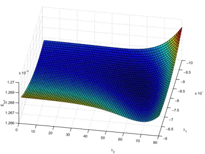
θ∗(Dt, λ) = arg min θ Cbt+1(θ, Dt, λ). (12) −10 −9.5 −9 −8.5 −8 −7.5 −7 −6.5 −6 x 10⁻³ 0 10 20 30 40 50 60 70 80 1.266 1.267 1.268 1.269 1.27 x 10⁻⁵ λ1 λ2 Et+1
Figure 1: Values of the sequential selection criterion for various values of the hyper-parameters. As in this particular case, the function is generally smooth. Here, the global minimum is obtained with λ1=−0.0085 and λ2= 60.
Note that there is a bijection between a parameterized function f and its set of parameters θ. Therefore, the above equation (12) is the same as the previous equation (7). For the application considered in this paper, the hyper-parameters λ are used for controlling training weights on past data points, i.e., giving a weight ws(t, λ) to the past observation at time s when minimizing the
training error up to time t, in equation (6). To weight the past data points, we have considered as an example a sigmoidal decay, with hyper-parameters λ1
ws(t, λ) =
1
1 + exp(−λ1(s− λ2)))
(13) This is a smooth version of the “abrupt transition” heuristic used in practice. To apply gradient-based optimization to the selection of the hyper-parameters (equation (9)), we will compute the gradient of the sequential cross-validation criterion bEt+1(equation (8)) with respect to the hyper-parameters:
∂ bEt+1 ∂λ λ=λ 0 = 1 t− M0 · t−1 X s=M0 ∂Q(θ, zs+1) ∂θ θ=θ∗(Ds,λ0) · ∂θ∗(Ds, λ) ∂λ λ=λ 0 . (14)
Basically, this involves looking at the minimum of bCt+1 with respect to the
parameter vector θ, for a given hyper-parameter vector λ (equation (12)), and then seeing how a change in λ influences the solution θ. The latter is rather unusual as we need to compute the derivative of the parameters θ with respect to the hyper-parameters λ.
Let us first differentiate the value of the derivative of the quadratic cost function with respect to the parameters. If f∈ F is affine, then Q is simply a quadratic function of the parameters and can thus be rewritten as
Q = a(λ) + b(λ)θ + 1 2θ
0H(λ)θ (15)
where λ is considered fixed and H(λ) is the symmetric positive-definite Hes-sian matrix of second derivatives of the training criterion with respect to the parameters. The computation of gradients with respect to hyper-parameters can also be performed for non-quadratic cost functions (Bengio, 1999) but in this paper, we only need to consider the simpler quadratic case. Differentiating Q with respect to θ, we obtain:
∂Q
∂θ = b(λ) + H(λ)θ (16)
We now need to obtain the values of b(λ) and H(λ). Since, b(λ) = ∂Q ∂θ θ=0 , (17)
we estimate b(λ) and H(λ) as:
bs(λ0) = − 1 s s X u=1 wu(s, λ0)· ˜xu· yu0 (18) Hs(λ0) = 1 s s X u=1 wu(s, λ0)· ˜xu· ˜x0u (19)
θ∗(Ds, λ0) =−Hs−1(λ0)· bs(λ0) (20)
And so, we are now able to compute the first term in equation (14): ∂Q(θ, zs+1) ∂θ θ=θ∗(Ds,λ0) = (θ∗(Ds, λ0)· ˜xs+1− ys+1)· ˜xs+1 (21)
Let us now derive the value of the derivative of the optimal parameters with respect to the hyper-parameters. Equation (20) provides us with an expression of the optimal parameters as a function of the hyper-parameters which we only need to differentiate to obtain the solution for the second term in the summation in equation (14): ∂θ∗(Ds, λ) ∂λ λ=λ0 =− ∂H −1(λ) ∂λ λ=λ0 · bs(λ0)− ∂b(λ) ∂λ λ=λ0 · Hs−1(λ0) (22)
The values of Hs−1(λ0) and bs(λ0) are given by equations (18) and (19).
Com-puting the derivative of these functions with respect to the hyper-parameters gives us the value of the two remaining terms.
∂b(λ) ∂λ λ=λ 0 = −1 s s X u=1 ∂wu(s, λ) ∂λ λ 0 · ˜xu· yu0 (23) ∂H(λ) ∂λ λ=λ 0 = 1 s s X u=1 ∂wu(s, λ) ∂λ λ 0 · ˜xu· ˜x0u (24) Noting that ∂H−1 ∂λ H + ∂H ∂λH −1= ∂H−1H ∂λ = ∂I ∂λ = 0 (25) We can isolate ∂H−1
∂λ as a function of known values:
∂H−1 ∂λ =−H
−1∂H
∂λH
−1 (26)
An even more efficient method using the Cholesky decomposition of the Hessian matrix can be found in (Bengio, 1999).
All four terms of equation (22) are known. We can then use the results of equations (22) and (21) to compute the derivative of the sequential cross-validation criterion with respect to the hyper-parameters (equation (14)). Then, using gradient descent will allow us to search the space of hyper-parameters in a continuous fashion towards a minimum (possibly local) of the sequential cross-validation criterion. Then, equation (11) provides us with an estimate of the generalization error of the whole process.
0 20 40 60 80 100 120 140 160 180 200 −1.5 −1 −0.5 0 0.5 1 1.5 Figure 2: Ratio yt
xt vs t from the generated data (noisy curve), and training
weights ws(200, λ) (smooth curve) found at the end of the sequence by
optimiz-ing the hyper-parameters λ1 and λ2.
4
Experiments on Artificial Data
We have tested the algorithm on artificially generated non-i.i.d. data with a single abrupt change in the input/output dependency at some point in the sequence. The single input/single output data sequence is generated by a Gaus-sian mixture for the inputs, and for the output given the input a left-to-right Input/Output Hidden Markov Model (Bengio & Frasconi, 1996). A sequence of T = 200 input/output pairs was generated. We set M0 = 25 and M = 50 (see equations (8) and (11)).
At time t = 80, when the model randomly switches to a state with a different distribution, the relation between the input and the output changes drastically, as seen in Figure 2 (with the ratio of output to input noisy curve).
The smooth curve in Figure 2 illustrates the values of the pattern weights after the 200 observations have been taken account of. Clearly, the algorithm has succeeded in identifying the input/output dependency change at time t = 80. Accordingly, those observations after time t = 80 are given weights close to 1 and observations before the transition point are given close to null weighting. Whereas research often concentrates on selecting, among a group of candidates, an optimal period of time which is to be used for all time-series of a given type and for the purpose of prediction, our algorithm selects this period automatically and independently for each time-series, thus recognizing that non-stationarities are unlikely to occur strictly simultaneously for all processes.
We compare a regular linear regression with a linear regression with three parameters: one parameter for the weight decay and two hyper-parameters (λ1 and λ2) to yield training weights on past data points with a
sigmoidal decay (equation (13)). The out-of-sample MSE for the regular linear regression is 3.97 whereas it is only 0.62 when the hyper-parameters are
opti-20 40 60 80 100 120 140 160 180 200 10−6 10−5 10−4 10−3 10−2 10−1 100 101 102
Figure 3: Out-of-sample squared loss for each time step t, for the ordinary re-gression (dashed) and rere-gression with optimized hyper-parameters (continuous).
mized. As shown in Figure 3, much better performance is obtained with the adaptive hyper-parameters, which allow to quickly recover from the change in distribution at t = 80. Between times t = 0 and t = 80, both errors closely map one another at low values. Then from time t = 80 to time t ≈ 90, both errors are are much higher (note the log-scale plot). Afterward, the model with hyper-parameters recovers and its errors drop back to values close to the ones obtained before the abrupt change. On the other side, the plain vanilla linear regression, stays stocked at high error values, unable to detect the change.
5
Experiments on Financial Time-Series
In this section, we describe experiments performed on financial data: predicting next month’s return first and second moment, for Canadian stocks. Let
rt= valuet/valuet−1− 1
be a discrete return series (the ratio of the value of an asset at time t over its value at time t− 1, which in the case of stocks includes dividends and capital gains). In these experiments, our goal is to make predictions on the first and second moment of rt+1, using information available at time t. These predictions
could be used in financial decision taking in various ways: for asset allocation (taking risks into account), for estimating risks, and for pricing derivatives (such as options, whose price depends on the second moment of the returns).
In the experiments we directly train our models to predict these two moments by minimizing the squared error, i.e., we are trying to learn Et[rt+1] and Et[r2t+1]
where Etdenotes the conditional expectation using information available up to
We have performed experiments on monthly returns and monthly squared returns of 473 stocks from the Toronto Stock Exchange (TSE) for which at least 98 months of data were available, the earliest starting in January 1976, and the latest data ending in December 1996.
5.1
Experimental Setup and Performance Measures
In all the experiments, we compare several models on the same data, and we use the sequential cross-validation criterion (equation (11)) to estimate generaliza-tion performance. For models with hyper-parameters, the “minimum” number of training points to evaluate parameters while hyper-parameters remained fixed was set to M0= 48 months (4 years). The minimum number of training points in order to train hyper-parameters was set to M = 72 months (6 years). In all other experiments using models without hyper-parameters, the “minimum” number of training points was set to M = 72. The out-of-sample MSE was computed for each stock. The results reported below concern the average MSE over all the 473 stocks. We have also estimated the variance across stocks of the MSE value, and the variance across stocks of the difference between the MSE for one model and the MSE for a reference model, as described below. Using the latter, we have tested the null hypothesis that two compared models have identical true generalization error.
For this purpose, we have used an estimate of variance that takes into account the autocorrelation of errors through time. Let et be a series of errors (e.g.
squared prediction error) with sample mean ¯e. ¯ e = 1 n n X t=1 et (27)
We are interested in estimating its variance: V ar[¯e] = 1 n2 n X t=1 n X t0=1 Cov(et, et0). (28)
Since we are dealing with a time-series and because we do not know how to estimate independently and reliably all the above covariances, we will assume that the error series is covariance-stationary and that the covariance dies out as |t−t0| increases. This can be verified empirically by drawing the autocorrelation
function of the etseries. The covariance stationarity implies that
Cov(et, et0) = γ|t−t0|, (29)
where the γ’s are estimated from the sample covariances:
ˆ γk= 1 n n−k X t=1 (et− ¯e)(et+k− ¯e) (30)
An unbiased and convergent estimator of this variance is thus the follow-ing (Priestley, 1981):
d V ar[¯e] = 1 n ˆγ0+ 2· m X k=1 (1− k/m)ˆγk ! , (31)
where limn→∞m =∞ and limn→∞m/n = 0: we have used m =√n.
Because there are generally strong dependencies between the errors of differ-ent models, we have found that much better estimates of variance were obtained by analyzing the differences of squared errors, rather than computing a variance separately for each average:
V ar[¯eA− ¯eB] = V ar[¯eA] + V ar[¯eB]
− 2Cov[¯eA, ¯eB] (32)
In the tables below we give the p-value of the null hypothesis that a model is not better than the reference model, using a normal approximation for the differences in average sequence errors.
5.2
Models Compared in the Experiments
The following models have been considered in the comparative experiments (note the “short name”, in bold below, used in the tables):
• Constant model: this is the reference or naive model, which has 1 free parameter, the historical average of the past and current output observa-tions.
• Linear 1 model is a linear regression with 1 input, which is the current value ytof the output variable yt+1; it has 2 free parameters.
• Linear 2 model is Linear 1 model with an extra input which is the aver-age over the last 6 months of the output variable; it has 3 free parameters. • Linear 4 model is Linear 2 model, with two extra inputs: the value of the output variable at the previous time step yt−1and the average over the
last 6 time steps of the return; this model was only used for the squared return prediction experiments; it has 5 free parameters.
• ARMA(p,q) model is a recurrent model of orders p (auto-regressive re-currences) and q (moving average lags). It has 1+p+q free parameters; we have tried the following combinations of p and q: (1,1),(2,1),(1,2),(2,2). • Hyper Constant model is the Constant model with weights on the past
data (learned with the hyper-parameters); there is 1 free parameter and 2 hyper-parameters.
• Hyper Linear 1 model is the Linear 1 model with weights on the past data; there are 2 free parameters and 2 hyper-parameters.
5.3
Experimental Results
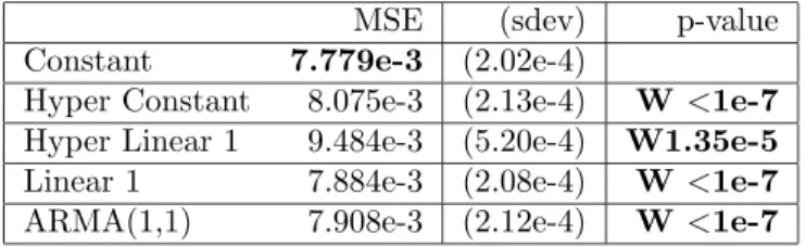
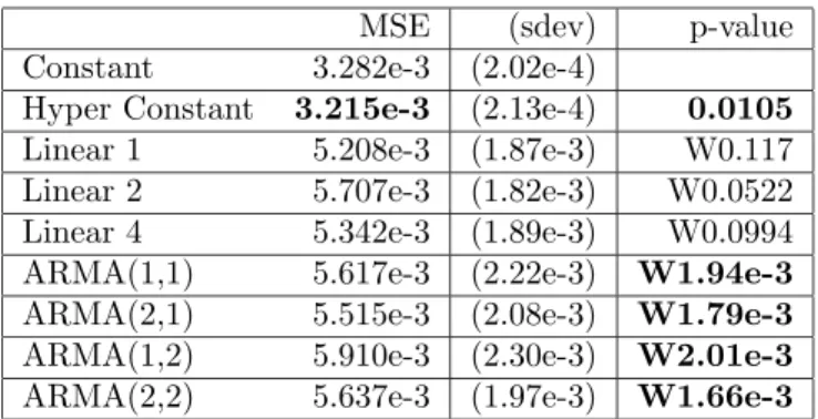
The results on predicting the first moment of next month’s stocks returns are given in table 1. Note that the p-values are one-sided but that we do two different tests depending on whether the tested model average error is less or greater than the reference (Constant model). In the latter case there is a “W” in the p-value column, indicating that the performance is worse than the reference. Significant results at the 5% level are indicated with a bold p-value. The lowest error over all the models is indicated by a bold MSE. For the first moment, the constant model significantly beats all the others. The results on predicting the second moment are given in table 2. The constant model with hyper-parameters significantly beats all the others.
MSE (sdev) p-value
Constant 7.779e-3 (2.02e-4)
Hyper Constant 8.075e-3 (2.13e-4) W <1e-7 Hyper Linear 1 9.484e-3 (5.20e-4) W1.35e-5 Linear 1 7.884e-3 (2.08e-4) W <1e-7 ARMA(1,1) 7.908e-3 (2.12e-4) W <1e-7
Table 1: Results of experiments on predicting one-month ahead stocks returns using a variety of models. The average out-of-sample squared error times 0.5 (MSE) over all the assets are given, with estimated standard deviation of the average in parentheses, and p-value of the null hypothesis of no difference with the Constant model. A “W” means that the alternative hypothesis is that the model is WORSE than the constant model. All the models are significantly worse than the Constant model.
6
Conclusions
In this paper we have achieved the following: (1) We have introduced an exten-sion of cross-validation, called sequential cross-validation as a model selec-tion criterion for possibly non-i.i.d. data. (2) We have applied the method for optimizing hyper-parameters introduced in (Bengio, 1999) to the special case of capturing abrupt changes in non-stationary data: 2 hyper-parameters control the weight on each past time step. (3) We have tested the method on artificial data, showing that when there is such an abrupt change, the regression is much improved by using and optimizing the hyper-parameters. (4) We have tested the method on financial returns data to predict the first and second moment of next month’s return for individual stocks. The specific conclusions of these experiments are the following: On estimating the conditional expectation of stock returns, the constant model significantly beats all the tested models, in-cluding linear and ARMA models. On estimating the conditional expectation of the squared return (which can be used to predict volatility), the constant
mod-MSE (sdev) p-value Constant 3.282e-3 (2.02e-4)
Hyper Constant 3.215e-3 (2.13e-4) 0.0105 Linear 1 5.208e-3 (1.87e-3) W0.117 Linear 2 5.707e-3 (1.82e-3) W0.0522 Linear 4 5.342e-3 (1.89e-3) W0.0994 ARMA(1,1) 5.617e-3 (2.22e-3) W1.94e-3 ARMA(2,1) 5.515e-3 (2.08e-3) W1.79e-3 ARMA(1,2) 5.910e-3 (2.30e-3) W2.01e-3 ARMA(2,2) 5.637e-3 (1.97e-3) W1.66e-3
Table 2: Results of experiments on predicting one-month ahead stocks squared returns using a variety of models. The average out-of-sample squared error times 0.5 (MSE) over all the assets are given, with estimated standard deviation of the average in parentheses, and p-value of the null hypothesis of no difference with the Constant model. A “W” means that the alternative hypothesis is that the model is WORSE than the constant model. The Hyper Constant model is significantly better than all the others while the ARMA models are all significantly worse than the Constant reference.
el with hyper-parameters to handle non-stationarities beats the other models, with a p-value of 1%.
What remains to be done, in the direction of research that we have ex-plored here? In our experiments we have found that the estimates of the hyper-parameters was very sensitive to the data, probably because of the variance of the cross-validation criterion, so better results might be obtained by using a less noisy model selection criterion. It would also be interesting to see if the signif-icant improvements that we have found for Canadian stocks can be observed on other markets, and if these predictions could be used to improve specific decisions concerning those stocks (such as for trading options).
References
Akaike, H. (1974). A new look at the statistical model identification. IEEE Transactions on Automatic Control, AC-19 (6), 716–728.
Bengio, Y. (1999). Continuous optimization of hyper-parameters. Tech. rep. 1144, D´epartement d’informatique et recherche op´erationnelle, Universit´e de Montr´eal.
Bengio, Y., & Frasconi, P. (1996). Input/Output HMMs for sequence processing. IEEE Transactions on Neural Networks, 7 (5), 1231–1249.
Craven, P., & Wahba, G. (1979). Smoothing noisy data with spline functions. Numerical Mathematics, 31, 377–403.
Evans, W., Rajagopalan, S., & Vazirani, U. (1993). Choosing a reliable hy-pothesis. In Proceedings of the 6th Annual Conference on Computational Learning Theory, pp. 269–276 Santa Cruz, CA, USA. ACM Press. Littlestone, N., & Warmuth, M. (1994). The weighted majority algorithm.
Information and Computation, 108 (2), 212–261.
Priestley, M. (1981). Spectral Analysis and Time Series, Vol.1: Univariate Series. Academic Press.
Tikhonov, A., & Arsenin, V. (1977). Solutions of Ill-posed Problems. W.H. Winston, Washington D.C.