PASSIVE, BROAD-BAND SEISMIC MEASUREMENTS FOR
GEOTHERMAL EXPLORATION : THE GAPSS EXPERIMENT
Davide Piccinini
1, Gilberto Saccorotti
1, Francesco Mazzarini
1, Maria Zupo
1,
Marco Capello
1, Giovanni Musumeci
1,2, Lena Cauchie
1,3and Claudio Chiarabba
41 Istituto Nazionale di Geofisica e Vulcanologia, sezione Pisa, Italy
2 Università di Pisa, Dipartimento di Scienze della Terra, Italy
3 University College of Dublin – School of Geological Sciences, Dublin, Ireland.
4 Istituto Nazionale di Geofisica e Vulcanologia, sezione CNT-Roma, Italy
Keywords: Larderello, Seismicity,
ABSTRACT
Passive seismological imaging techniques based on
either transient (earthquakes) or sustained
(background noise) signals can provide detailed
descriptions of subsurface attributes as seismic
velocity, attenuation, and anisotropy. However, the
correspondence between these parameters and the
physical properties of crustal fluids is still ambiguous.
Moreover, the resolving capabilities and condition of
applicability of emerging techniques such as the
Ambient Noise Tomography are still to be investigated
thoroughly. Following these arguments, a specific
project (GAPSS-Geothermal Area Passive Seismic
Sources) was planned, in order to test passive
exploration methods on a well-known geothermal
area, namely the Larderello-Travale Geothermal Field
(LTGF). This geothermal area is located in the western
part of Tuscany (Italy), and it is the most ancient
geothermal power field of the world. Heat flow in this
area can reach local peaks of 1000 mW/m3. The deep
explorations in this area showed a deeper reservoir
(3000 to 4000 m depth) located within the
metamorphic rocks in the contact aureole of the
Pliocene-Quaternary granites [Bertini et al., 2006]; it
is characterized by a wide negative gravimetric
anomaly, interpreted as partially molten granite at
temperatures of 800°C [Bottinga and Weill, 1970].
From seismic surveys the marker K (pressurized
horizons) was found at depths between 3 and 7 km
[Batini and Nicolich, 1984; Bertini et al., 2006]. The
structural grain of the geothermal field is characterized
by N-W trending and N-E dipping normal faults
whose activity lasts since the Pliocene [Brogi et al.,
2003].
GAPSS is ongoing since early May, 2012, and it
consists of 12 temporary seismic stations,
complemented by two permanent stations from the
National Seismic Network of Italy. The resulting array
has an aperture of about 50 Km, with average station
spacing of 10 Km. Stations are equipped with either
broadband (40s and 120s) or intermediate-period (5s),
3-components seismometers.
LTGF is seismically active. During the first 2 months
of measurements, we located about 250 earthquakes,
with a peak rate of up to 40 shocks/day. Preliminary
results from analysis of these signals include: (I) a
study of local micro-earthquakes remotely triggered
by the surface waves from the Po Plain main-shock
(May 20,2012). Results suggest a triggering process
most likely related to the Coulomb failure of faults
kept close to rupture by elevated fluid pore pressure.
(ii) The detailed location of clustered
microearthquakes from inversion of differential times,
thus obtaining a detailed picture of fracture geometry.
(ii) Seismic noise analysis, thus far mostly aimed at
elucidating the directional properties of the noise
wavefield over the microseismic (0.1-0.5 Hz)
frequency band.
1. INTRODUCTION
The GAPSS (Geothermal Area Passive Seismic Sources) is a project of the Istituto Nazionale di Geofisica e Vulcanologia (INGV hereinafter) aimed at testing robustness and conditions of applicability of passive seismic techniques for the evaluation of the geothermal potential. For this purpose, we selected as a test site the Larderello-Travale geothermal field (Tuscany, Italy, hereinafter LTGF), an area for which independent geological and geophysical data allow for a detailed imaging of the subsurface rock properties.
Like the majority of geothermal areas, the background seismicity at LTGF is significantly higher than the surrounding region. The GAPSS experiment consists of a large-aperture seismic array composed by 11 broad-band sensors, which complement two permanent seismic stations operated in the area as a part of the National Seismic Network (RSN).
Besides the characterization of the seismic release of the LTGF, our purpose is to investigate the geothermal field applying cost-effective passive seismic techniques, such as local earthquake tomography, attenuation tomography, shear wave splitting analysis and surface-wave dispersion from noise correlation analysis.
Local earthquake seismic tomography use earthquakes instead of seismic sources and, from the inversion of the P and S-wave arrival times, allow for imaging the velocity structure of those portions of the crust illuminated by seismic rays. In addition, a number of recent studies focused on attenuation (the inverse of Q, the quality factor) derived by spectral analyses of compressional and shear waves of local earthquakes. Variations in Q may be interpreted in terms of variations in the degree of water saturation, pressure, temperature, the presence of gas, partial melting and degree of compositional heterogeneity. The joint interpretation of P- and S-wave velocity and attenuation models is expected to provide a bright imaging of the investigated volume; while P-wave velocities are mostly controlled by lithology, Qp and [Vp/Vs, Qp/Qs] ratios reveal the presence and the physical state of fluids within the uppermost crust (Chiarabba et al., 2009, Piccinini et al., 2010).
Shear-wave splitting due to aligned cracks in the crust have been observed world-wide and occurs in a variety of tectonic settings and data gathering experiments, ranging from earthquake monitoring (Pastori et al, 2012, and references therein) to controlled source seismic profiling. It has been recognized that the polarization of the fast split shear-wave is usually parallel to the local strike of cracks. Further, the time delay between the fast and the slow shear waves is directly related to the degree of anisotropy induced in the medium by aligned cracks (Crampin 1987, Crampin and Lovell 1991). Therefore, the recording and inversion of shear wave splitting is an important diagnostic tool for finding the direction and density of subsurface cracks in energy reservoirs (Muller, 1991).
Noise correlation analysis starts with Aki (1957), who defined a procedure to exploit the seismic noise to retrieve, from its autocorrelation function, the dispersion curve of the surface waves and the S-wave velocities for different depths in the subsurface of a seismic station. Claerbout (1968) proposed using the auto-correlation of the ambient noise to derive the reflection seismic response and hence to obtain images of the Earth's interior. The instrumental improvements of the last years (which ensure a continuous recording over broad frequency bands) marked the start of a renewal of this subject, which found many different applications in seismology: from large-scale, passive seismic imaging (e.g., Shapiro et al., 2005), to seismic exploration (e.g., Draganov et al., 2007).
This paper describes the methods and the preliminary results obtained from the analysis of the data collected during the first 3 months of the experiment (May-July 2012).
2. LARDERELLO-TRAVALE GEOTHERMAL
FIELD: GEOLOGICAL OUTLINE
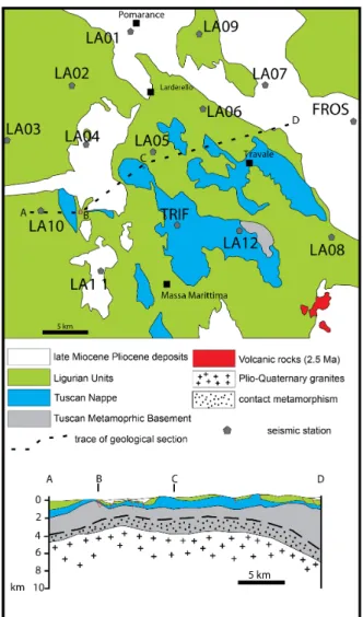
The Larderello geothermal field (Fig. 1) is a large area of the Northern Apennines where, since the Pliocene, the emplacement of shallow-level intrusions has led to the development of diffuse thermal aureoles and associated hydrothermal systems, both sampled by several wells performed for geothermal exploitation (Gianelli et al., 1997; Carella et al., 2000; Gianelli and Ruggeri, 2002; Musumeci et al., 2002). Larderello is a steam-dominated geothermal field and was used for commercial production of electricity since 1913. The whole geothermal area is about 400 km2 and has a production of more than 1000 kg/s of super-heated steam, with a running capacity of about 700 MW (Cappetti and Ceppatelli, 2005). Hydrothermal systems, occurring at depths ranging between 500 and 4000 m, show an evolution from an early stage, coeval with granitic intrusions,
dominated by magmatic and metamorphic fluids, to the present-day stage dominated by meteoric fluids. The growth of hydrothermal mineral assemblages within brittle veins and/or fracture systems is regarded as evidence of fluid circulation coeval with repeated episodes of brittle deformation.
Figure 1: Geological sketch map of the
Larderello-Travale Geothermal field after Bertini et al.,
2006, with location of both permanent and
temporary seismic stations operated in the
frame of GAPSS experiment.
The tectonic structure of the geothermal field consists of a stack of Alpine tectonic units, namely the Ligurian Unit and the Tuscan Nappe (Fig. 1), which overlie the Tuscan Metamorphic Complex. The latter is a buried complex of low-grade metamorphic units made up of terrigenous and carbonatic successions of Permian-Triassic (Musumeci et al., 2002) and Palaeozoic age rocks (Batini et al., 1983). Shallow-level emplacement of Pliocene intrusive rocks in the metamorphic tectonic units led to the development of broad low pressure – high temperature (0.15-0.2 GPa – 500° -650° C) contact aureoles with development of medium to high grade hornfels rocks and associated hydrothermal systems (Cavaretta et al., 1982; Carella et al., 2000; Gianelli and Ruggeri, 2002; Musumeci et al., 2002). A noteworthy feature of the geothermal field is the occurrence of seismic reflectors, named the K-horizon and H-horizon (Bertini et al., 2006 and references therein). The K-horizon occurs in
the 3 - 6 km depth range, at the top of Quaternary granites
(Batini et al., 1978, 1983). This horizon is characterized by a strong amplitude signal of bright-spot type, suggesting the occurrence of fluids (magmatic, metamorphic and mixed fluids) hosted within cracks and/or micro-cracks. On this ground the K-horizon has been considered as to be the top of a fluid-rich level (Batini et al., 1983; Gianelli et al., 1997) that cyclically underwent to episodes of fluid overpressure also testified by concentration of seismic activity of low magnitudo (Bertini et al. 2006). The culmination of the K-horizon at a depth of nearly 3000 m is in the Lago area (south of Larderello; Fig. 1) where the K-horizon was reached by the San Pompeo 2 well, which exploded when the K-horizon was drilled. The overlying H-horizon occurs at shallower depth (2-4 km) in correspondence of the contact aureole of the Pliocene granites and it is regarded as a fossil K-horizon (Bertini et al., 2006).
Main faults in the Larderello geothermal fields are normal faults associated with the latest extensional episode which is lasting since late Pliocene. Faulting affects very shallow crustal levels (c.a. 1 km depth) with major NW-trending, NE-dipping and NE-trending normal to strike-slip steeply dipping faults (Brogi et al., 2003).
3. The experiment
LTGF is seismically active, and is routinely monitored by a seismic network from ENEL, the power company that operates the geothermal plants. ENEL data, however, are not accessible. Public permanent stations in the area are in operation only since mid 2010, when two instruments (TRIF and FROS; see Fig.1) were installed as a part of INGV's RSN. By early May, 2012, we complemented the two permanent stations with eleven temporary instruments. The resulting array has an aperture of about 50 km and average station spacing around 10km (Fig.1); the acquisition is foreseen to extend throughout a 15-months time interval. The geometry of the network has been designed in order to obtain a complete azimuthal coverage of the whole geothermal area. The two permanent stations are equipped with GAIA2 digitizers, connected with Nanometrics Trillium 40s broad-band seismometer (flat response over the 0.025-50 Hz frequency range). Each mobile station, named as LA[01-12], is equipped with a Reftek RT-130 recorder, acquiring data at 125 samples/second/channel with a nominal dynamic range of 24 bits. Ten recordings sites are equipped with Trillium SP120-compact broad-band, three-component seismometers, depicting a flat amplitude response over the 0.00833Hz-50Hz frequency range. The remaining two sites are equipped with Lennartz LE3D-5s, three-component seismometers, with flat response over the 0.2-50Hz frequency range. Both recorders and seismometers are provided by the RE.MO. (Mobile Seismic Network) facility at INGV-CNT.
4. Earthquake Data
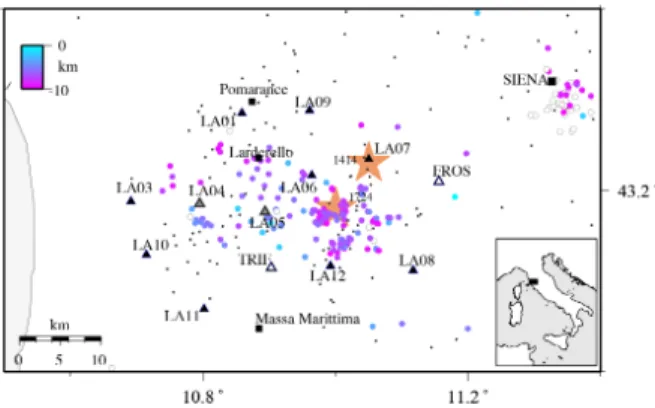
In Figure 2 we show the instrumental seismicity recorded and located during the first three months of the GAPSS experiment. Seismicity is shallow (Z < 10 km) and widespread throughout the geothermal area. Hypocentral depths follow the k-horizon top (see Figure 1), and they are shallower in the southernmost part of the geothermal field. Moving toward north and east, seismicity gets deeper. In the
SE sector of the study area, two clusters of epicenters are evident. This is the same area which was affected by the two most significant (M > 5) historical earthquakes (1414, M=5.6; 1724, M=5.4, http://emidius.mi.ingv.it/DBMI11/ ).
Figure 2: Map of seismicity recorded during the
first three months of the GAPSS experiment
(filled, colored circles). The color of the
symbols indicate source depth, according to
the color scale at the upper left. White dots
are those hypocenters located at depth larger
than 10 km. Temporary GAPSS stations are
marked by black triangles and are all
equipped with broadband seismic sensors,
except for two extended-period seismometers
(light gray triangles). Open triangles mark
the two permanent RSN stations. Seismicity
located by RSN is indicated by gray dots.
In Figure 3 we show basic statistic for the 257 best located events, with horizontal and vertical errors lower than 2 km. Although most of the seismicity occurred within the GAPSS network, we also located a small cluster of events occurred few tens of kilometers ENE off the study area (Fig. 2). This is highlighted in the Figure 3, panel (b) which shows a sharp peak of locations with azimuthal gaps greater than 300°. Note the strong difference between the P and S-wave residuals [panels g and h], and in particular the slight bimodal distribution of the S-wave residuals, likely related to a un-modeled, strong lateral heterogeneity of the S wave model. To improve the hypocentral location also with the use of the S-wave arrival times, an average Vp/Vs ratio is computed. The “modified Wadati diagram” provides an estimate of Vp/Vs of 1.73 similar to those found by previous studies for the same area (De Matteis et al., 2007). Moment magnitude is estimated by fitting the low-frequency level of the displacement spectra, span between 0.5 and 2.3 with a rate of about 5 events per day. Episodic accelerations of this rate are clearly visible in the time series plot. Excluding earthquakes occurred outside the network, we then derive the frequency distribution of magnitudes (Gutenberg-Richter relationship [GR]; Fig.3l). The completeness magnitude for the catalogue is Mw=1.4 (+/- 0.11) and the b-value is 1.47 (+/- 0.22), thus significantly higher than those usually observed in seismically active regions worldwide. The b-value is the slope of the straight line fitting the GR relationship at magnitudes larger than the completeness magnitude. The former is inversely proportional to the mean magnitude, given the minimum observed magnitude. Thus,mapping the b-value is equivalent to mapping the mean magnitude, i.e. the mean crack length. It has to be noted that stress, material properties, temperature, or any combination of these parameters can modulate the frequency-magnitude distribution or the average crack size in the crust. Thus b-value anomalies in different tectonic environments may be interpreted in different ways.
Figure 3: Location statistics for the 257
earthquakes recorded by the GAPSS
deployment during the May-July, 2012, time
interval. (a) Number of phases (P, S) used for
locations. (b) Azimuthal gap. (c)
Root-Mean-Square of travel time residuals. (d) Temporal
evolution of moment magnitudes. (e, f)
Horizontal and vertical, respectively,
location errors. (g, h) Travel time residuals
for P- and S-waves. (i) Modified Wadati
diagram for estimation of Vp/Vs ratio. (l)
Gutenberg-Richter relationship and
magnitude-of-completeness determination.
The vertical gray lines in panels (c, e, f)
represent the 90% percentile of individual
distributions.
5. Noise Analysis
One of the most significant finding of modern seismology concerns the observation that the Green's function between two locations can be extracted from the diffuse noise field using a simple field-to-field correlation function (Noise Correlation Function, NCF; Snieder, 2004). Assuming that the noise wavefield is mainly constituted by Rayleigh waves, this implies the possibility of deriving the dispersion characteristics, and hence a velocity structure, over a broad range of wavelengths. Crucial to the application of these
methodologies are the assumptions regardingthe diffuse and stationary character of the noise wavefield.
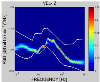
Figure 4: Probability density function of spectral
power for three months of recordings at the
vertical component of station LA12 (see Figs.
1 and 2). Individual spectra have been
obtained using Welch's method applied to
600-s-long windows spanning 1-hour of data.
Figure 4 illustrate the probability density function
(McNamara and Buland, 1995) of the noise power spectra. Data are from the vertical component of station LA12 (see Fig. 1), and span three months of continuous recording. As expected, noise spectra are dominated by a major peak at frequencies around ~0.3 Hz, associated with secondary microseism.
Figure 5:
Polar representation of wave
backazimuths and ray parameters obtained
from conventional beam-forming over the
0.05-0.5 Hz frequency band. Data are for the
21 of May, 2012.
In order to evaluate the structure of the noise wavefield, we first use a deterministic procedure, namely a conventional,
frequency-domain beamformer (e.g., Abrahmson and Bolt,
1987). Under a plain-wave approximation, we calculate slowness spectra over the 0.1- 0.5 Hz frequency band, using 600s-long time window sliding along the vertical-component seismograms. Figure 5 shows wave backazimuths derived from the peaks of slowness spectra for 1 complete day of recording. Over that time scale, the noise wavefield is markedly directional. The dominant backazimuths are associated with waves coming from the southern Thyrrenian sea, propagating with velocities (~3 km/s) which are consistent with Rayleigh waves. Secondary contributions are from waves coming from the NW, likely related to swells in the Ligurian Sea.
As mentioned above, the correspondence between the Green's function and the NCF is based upon an assumption of diffuse noise wavefield (Snieder, 2004). In general, this approximation holds once the NCF is obtained after stacking over long time intervals. Our procedure for calculating the NCF thus begins with the signal preconditioning, i.e. demeaning, detrending, tapering and instrument correction of day-long recordings. These time-domain signals are then normalised according to their local absolute values (RAM-Running absolute mean; Bensen et al., 2007), and then Fourier-transformed. After spectral whitening, signals are brought back into the time domain, and used for calculating the cross-correlation functions over 600-s-long time intervals. These function are eventually stacked to produce a daily estimates of the NCF.
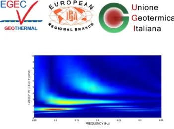
Figure 6 shows sample daily correlation functions for
station pairs LA03-LA08 for 40 consecutive days of recording. These functions show a marked daily variability, likely related to corresponding changes in marine climate. The stacked correlation function (top trace), exhibits however a certain degree of symmetry, thus suggesting that once averaged over longer time interval, the noise wavefield may be approximated to a random, diffuse field. Application of FTAN analysis to the stacked correlation curve allow retrieving a dispersion map, where the power of the Green's function is expressed as a function of frequency and group velocity (Fig. 7).
Figure 6: Daily Noise Correlation Functions (NCF)
for station pair LA03-LA08, throughout the
May 15 – July 20 time interval. The top trace
is the stack of the individual, daily NCFs.
Figure 7: Results from FTAN analysis: The power
of the NCF is contoured as a function of
frequency and velocity.
3. CONCLUSIONS
IIn this paper we presented a few preliminary results
obtained from analysis of data collected during the
early stages of the GAPSS experiment. The diffuse
character of the seismicity (Fig. 2) and its significant
rate (Fig. 3) indicate that, by the end of the
experiment, ray coverage will be sufficiently dense for
retrieving detailed tomographic imaging of both
attenuation and velocity parameters. On the other side,
the analysis of seismic background noise suggests that
the conditions of diffuse noise wavefield may be
attained over relatively short (few months) time
intervals, thus opening the way to the retrieval of
Rayleigh waves Green's functions and associated
group and phase velocities dispersion curves. Though
needing acquisition surveys extended over long time
span, the above considerations indicate that passive
seismological methods may offer a cost-effective
complement to the information gained through active
methods.
REFERENCES
Abrahamson, N. A. , and B.A. Bolt (1987). Array
analysis and synthesis mapping of strong seismic
motion, in Seismic Strong Motion Synthetics,
B.A. Bolt (editor), Academic Press Inc., New
York NY.
Aki K., (1957). Space and time spectra of stationary
stochastic waves with special reference to
microtremors. Bull. Earthq. Res. Inst. 35, 415-456.
Batini, F., Burgassi, P.D., Cameli, G.M., Nicolich, R.
and Squarci, P., 1978. Contribution to the study of
the deep lithospheric profiles: deep reflecting
horizons in Larderello-Travale geothermal field.
Mem.Soc. Geol. Ital., 19, 477-484.
Batini, F., Bertini, G., Gianelli, G., Pandeli, E. and
Puxeddu, M., 1983. Deep structure of the
Larderello field: contribution from recent
geophysical and geological data. Soc. Geol. Ital.
Mem., 25, 219–235.
Bensen, G. D., Ritzwoller, M. H., Barmin, M. P.,
Levshin, A. L., Lin, F., Moschetti, M. P., Shapiro,
N. M., and Y. Yang (2007). Processing seismic
ambient noise data to obtain reliable broad-band
surface wave dispersion measurements. Geophys.
J. Intern. 169, 1239-1260. DOI:
10.1111/j.1365-246X.2007.03374.x
Bertini, G., Casini, M., Gianelli, G. and Pandeli, E.,
2006. Geological structures of a long-living
geothermal system, Larderello, Italy. Terra Nova,
18,
163–169,
doi:10.1111/j.1365-3121.2006.00676.x.
Brogi, A., Lazzarotto, A., Liotta, B. and Ranalli, G.,
2003. Extensional shear zones as imaged by
reflection seismic lines: the Larderello geothermal
field (central Italy). Tectonophysics, 363, 127–139.
Chiarabba C., D. Piccinini, P. De Gori, 2009. Velocity
and attenuation tomography of the Umbria Marche
1997 fault system: Evidence of a fluid-governed
seismic sequence, Tectonophysics, Volume 476,
Issues 1–2, 15 October 2009, Pages 73-84, ISSN
0040-1951, 10.1016/j.tecto.2009.04.004.
Cappetti, G., Ceppatelli, L., 2005. Geothermal power
generation in Italy: 2000–2004 update report. In:
Proceedings 2005 World Geothermal Congress,
Antalia, Turkey.
Carella, M., Fulignati, P., Musumeci, G. and Sbrana,
A., 2000. Metamorphic consequences of Neogene
thermal anomaly in the northern Apennines
(Radicondoli – Travale area, Larderello geothermal
field, Italy). Geodinamica Acta, 13, 345–366.
Cavarretta, G., Gianelli, G. and Puxeddu, M., 1982.
Formation of authigenic minerals and their use as
indicators of physico-chemical parameters of the
fluid in the Larderello-Travale geothermal field.
Economic Geology, 77, 1071–1084.
Claerbout J. F., (1968). Synthesis of a layered medium
from its acoustic transmission response. Geophys.
33, 264-269.
Crampin, S., 1987. Crack porosity and alignment from
shear-wave VSPs, in Shear-wave Exploration, eds.
S.H. Danbom & S.N. Domenico, Geophysical
Developments, SEG Special Publ., 227-251.
Crampin, S. & Lovell. J.H., 1991. A decade of
shear-wave splitting in the Earth's crust: what does it
mean? what use can we make of it? and what
should we do next? in Proc. 4th Int. Workshop on
Seismic Anisotropy, Edinburgh, 1990, eds. J.H.
Lovell & S. Crampin, Geophys. J. Int., 107,
387-407.
Draganov D., Campman X., Thorbecke J., Verdel A.,
Wapenaar K., (2007). Reflection from ambient
seismic noise. Geophys. 74, 5, A63-A67.
Gianelli, G., Manzella, A. and Puxeddu, M., 1997.
Crustal models of the geothermal areas of southern
Tuscany (Italy). Tectonophysics, 281, 221–239.
Gianelli, G. and Ruggieri, G., 2002. Evidence of a
contact metamorphic aureole with
high-temperature metasomatism in the deepest part of
the active geothermal field of Larderello, Italy.
Geothermics, 31, 443–474.
McNamara, D. E. and R.P. Buland, 2004.Ambient
Noise Levels in the Continental United States,
Bull. Seism. Soc. Am., 94, 1517-1527.
Mueller, M. C., 1991, Prediction of lateral variability
in fracture intensity using multicomponent
shear-wave surface seismic as a precursor to horizontal
drilling: Geophys. J. Intemat., 107,409-415.
Musumeci, G., Bocini, L. and Corsi, R., 2002. Alpine
tectonothermal evolution of the Tuscan
Metamorphic Complex in the Larderello
geothermal field (northern Apennines, Italy).
Journal of the Geological Society,
London, 159, 443-456,
doi:10.1144/0016-764901-084.
Piccinini D, Di Bona M, Lucente F P, Levin V, Park J
(2010). Seismic attenuation and mantle wedge
temperature in the northern Apennines subduction
zone (Italy) from teleseismic body wave spectra.
Journal Of Geophysical Research, vol. 115, ISSN:
0148-0227, doi: 10.1029/2009JB007180
Shapiro N.M., Campillo M., Stehly L., Ritzwoller
M.H., (2005). High-resolution surface wave
tomography from ambient seismic noise. Science
307, 1615-1617
Snieder R. (2004). Extracting the Green’s function
from the correlation of coda waves: a derivation
based on stationary phase, Phys. Rev. E, 69, 1–8.
Acknowledgements
Mobile instruments used in the experiment have been provided by ReMo., the seismological instrument facility at INGV-CNT.