Synchronization and Balancing on the
N-Torus ?
L. Scardovi ∗ , A. Sarlette , R. Sepulchre
Department of Electrical Engineering and Computer Science, University of Li`ege, Montefiore Institute, B-4000 Li`ege, Belgium
Abstract
In this paper, we study the behavior of a network of N agents, each evolving on the circle. We propose a novel algorithm that achieves synchronization or balancing in phase models under weak connectedness assumptions on the (possibly time-varying and unidirectional) communication graphs. The global convergence analysis on the
N -torus is a distinctive feature of the present work with respect to previous results
that have focused on convergence in the Euclidean space.
Key words: Synchronization, Distributed algorithms, Phase models, Consensus
algorithms, Stability
1 Introduction
Over the past decade, particular attention has been devoted to the study of collective problems where interacting agents must reach a common objective under information and communication constraints. These problems arise in a
? This paper presents research results of the Belgian Programme on
Interuniver-sity Attraction Poles, initiated by the Belgian Federal Science Policy Office. The scientific responsibility rests with its authors.
∗ Corresponding author: Phone:+32 4 366 29 87, Fax:+32 4 366 29 89. Email addresses: [email protected] (L. Scardovi),
[email protected] (A. Sarlette), [email protected] (R. Sepulchre).
variety of disciplines including physics, biology, computer science and systems and control theory. Analysis and design efforts have been devoted to under-stand how a group of moving agents (e.g. flocks of birds, schools of fish or au-tonomous robots) can reach a consensus without an external reference and in a decentralized way. Applications include formation control of autonomous ve-hicles [2,14] and sensor networks [5,6]. In physics, synchronization phenomena in populations of coupled oscillators have received a lot of attention [4,15,16]. These phenomena have been studied mainly by means of phase models giv-ing rise to the celebrated Kuramoto model and in these last years the related dynamics have been investigated by means of system theoretic tools [12,3,8]. In those applications, the collective design can be formalized as the design of a decentralized algorithm for the collective optimization of a suitable cost func-tion characterizing a common objective [11]. The natural –e.g. gradient-based – optimization algorithms require all-to-all information exchange because the cost function depends on the entire state. In the present paper we call such algorithms global information algorithms. However the communication con-straints restrict the information available to a given agent at a given instant of time. In the present paper we call the algorithms that fulfill the communica-tion constraints local informacommunica-tion algorithms. The optimizacommunica-tion based design of local information algorithms either requires to constrain the cost function in accordance with the communication constraints or to approximate the global information algorithm with a local one. The first solution –adapting the cost function – is systematic but challenging when the communication constraints are uncertain and might change over time, which is the typical situation en-countered in practice. The present paper focuses on the second solution, which consists in approximating the global information algorithm.
We focus on the distributed stabilization of a phase model in continuous and discrete time. Because each phase variable evolves on the circle S1, the total
state-space is the N−torus TN = S1× . . . × S1. The global convergence
analy-sis on the N-torus is a distinctive feature of the present work with respect to previous synchronization results [9],[8],[3] that have focused on convergence in the Euclidean space, considering the present problem either by local lineariza-tion or by restriclineariza-tion of the initial condilineariza-tions to a subdomain diffeomorphic to the Euclidean space.
of synchronization and balancing on the N-Torus. In Section 3 we review the problem of reaching a consensus in the Euclidean space in a distributed setting and in Section 4 a natural extension to the N-Torus is provided. Section 5 and Section 6 present local information algorithms and global convergence analysis of the proposed decentralized algorithms is established. Finally, in Section 7, we conclude with some observations and perspectives for future research.
2 Synchronization and balancing on the N-Torus
Consider N autonomous agents evolving on the circle, each agent is repre-sented by its state θk∈ S1, k = 1, . . . , N. The total state space is the N-torus
TN = S1× . . . × S1, we will indicate by θ ∈ TN the state of the overall system.
We consider algorithms that only use relative information such as phase differ-ences. The resulting state space is then the quotient shape space TN/S1 where
all states differing by a rigid rotation are identified. A synchronized state is a configuration in which all the agents lie at the same position on the circle. In contrast, a balanced state is reached when the agents are “dispersed” on the circle. The concept of synchronization and balancing is formalized by the definition of the centroid
pθ = 1 N N X k=1 eiθk = |p θ|eiψ ∈ C. (1)
The parameter |pθ| is a measure of synchrony of the phase variables θ. It is
maximal when all phases are synchronized (identical). It is minimal when the phases balance to result in a vanishing centroid. Hence synchronization and balancing correspond to maximizing or minimizing the cost function
V (θ) = N 2|pθ|
2. (2)
Its gradient is computed as ∂V ∂θk =< pθ, ieiθk >= 1 N N X j=1 sin(θj − θk) , (3)
where the inner product < ·, · > is defined by < z1, z2 >= Re{¯z1z2} for z1, z2 ∈
gradient algorithm associated to the cost function (2) is ˙θk = − K N N X j=1 sin(θj− θk) = −K < pθ, ieiθk >, (4)
for k = 1, . . . , N, where the sign of the parameter K determines a descent or ascent algorithm for the cost (2). We report here a result in [12] that provides a characterization of the critical points of (4):
Theorem 1 The potential V (θ) = N
2|pθ|2 reaches its unique minimum when
pθ = 0 (balancing) and its unique maximum when all phases are identical
(synchronization). All other critical points of V (θ) are isolated in the shape manifold TN/S1 and are saddle points. The phase model (4) forces
conver-gence of all solutions to the critical set of V (θ). If K < 0, then only the set of synchronized states is asymptotically stable and every other equilibrium is unstable. If K > 0, then only the set of balanced states is asymptotically stable and every other equilibrium is unstable. ¤ Because the dynamics (4) evolve in the shape manifold TN/S1, it is worth
noting that the conclusions of Theorem 1 are equivalently stated in a rotating frame, that is, for the phase model
˙θk= ω − K N N X j=1 sin(θj− θk) = ω − K < pθ, ieiθk >, ω ∈ R. (5)
This all-to-all model is the most frequently studied coupling in the literature of coupled oscillators [4,16,15]. It is a particular case of the celebrated Kuramoto model where each oscillator is modeled by a phase variable θk ∈ S1 that, in
the absence of coupling, obeys the trivial dynamics ˙θk = ωk where ωk is the
natural frequency of oscillator k. Its application in the context of collective stabilization of steered particles in the plane is discussed in [12]. It is also of interest to study the discrete-time counterpart of the continuous time model (4). To this end we interpret (4) as follows: when K < 0 each agent moves towards the centroid pθ, when K > 0 each agent moves away from the centroid
pθ. This interpretation suggests the discrete-time algorithm [10]
θk[t + 1] = arg
³
(1 − δk)eiθk[t]± δkpθ[t]
´
, δk ∈ (0, 1), k = 1, . . . , N. (6)
The update (6) amounts, for each particle, to moving towards the centroid (respectively away from it) in the complex plane and to project the result
onto the manifold S1 (see Fig.1). It is worth noting that (6) reduces to (4) as
δk→ 0, k = 1, . . . , N.
The algorithms (6) and (4) make use of all-to-all communication to calculate the centroid pθ that appears in the expression of the gradient (3). In a local
information algorithm, this average quantity must be replaced by local infor-mation that might change over time. The next section summarizes important results on this topic, when the state space is an Euclidean space.
N-Torus -Re 6 Im u θ1[t] u θ2[t] uθ3[t] b P H H Y ¯¯ ¯¯ ¯¯ e θ3[t+1] Complex plane -Re 6 Im u eiθ1[t] u eiθ2[t] ueiθ3[t] r pθ[t] ³ ³ )³³ ³ ³ bP
Fig. 1. Interpretation of (6) as a projection onto the manifold S1
(P , (1 − δk)eiθk[t]+ δ
kpθ[t])
3 Consensus in Euclidean space
In this section we recall some recent results about consensus algorithms in the Euclidean space. This Consensus problem, has received considerable attention in the recent years, see for instance [9,8,7,1].
Let G = (V, E, A) be a weighted digraph (directed graph) where V = {v1, . . . , vN}
is the set of nodes, E ⊆ V × V is the set of edges, and A is a weighted adja-cency matrix with nonnegative elements akj. The node indices belong to the
set of positive integers I , {1, . . . , N }. Assume that there are no self-cycles i.e. akk = 0, ∀ k ∈ I.
The graph Laplacian L associated to the graph G is defined as Lkj = P iaki, j = k −akj, j 6= k.
The k-th row of L is defined by Lk. The in-degree (respectively out-degree)
of node vk is defined as dink =
PN
j=1akj (respectively doutk =
PN
j=1ajk). The
digraph G is said to be balanced if the in-degree and the out-degree of each node are equal, that is,
X j akj = X j ajk, ∀ i ∈ I.
It is both of theoretical and practical interest to consider time-varying commu-nication topologies. For example, in a network of moving agents, some of the existing links can fail and new links can appear when other agents enter an ef-fective range of detection. In the following we assume that the communication topology is described by a time-varying graph G(t) = (V, E(t), A(t)), where A(t) is piece-wise continuous and bounded and akj(t) ∈ {0} ∪ [β, γ], ∀ k, j, for
some finite scalars 0 < β ≤ γ and for all t ≥ 0. The set of neighbors of node vk at time t is denoted by Nk(t) , {vj ∈ V : akj(t) ≥ β}. We recall two
defin-itions that characterize the concept of uniform connectivity for time-varying graphs.
Definition 1 Consider a graph G(t) = (V, E(t), A(t)). A node vk is said to
be connected to node vj (vj 6= vi) in the interval I = [ta, tb] if there is a path
from vk to vj which respects the orientation of the edges for the directed graph
(N , ∪t∈IE(t),
R
IA(τ )dτ ).
Definition 2 G(t) is said to be uniformly connected if there exists T > 0 such that for all t there is one node connected with all the other nodes across [t, t + T ].
Consider a group of N agents with state xk ∈ X, where X is an Euclidean
space. The communication between the N-agents is defined by the graph G: each agent can sense only the neighboring agents, i.e. agent j receives infor-mation from agent i iff i ∈ Nj(t). We use the notation k ∼ j to indicate
the presence of a communication link from agent j to agent k, i.e. k ∼ j iff vj ∈ Nk.
In continuous time, we consider the continuous dynamics ˙xk=
X
k∼j
akj(t)(xj − xk), ∀k ∈ I. (7)
Using the Laplacian definition, (7) can be equivalently expressed as
˙x = −L(t) x. (8)
A discrete time version of (8) is
x[t + 1] = x[t] − ε[t]L[t]x[t], ε = diag(ε1, ε2, ..εN), εk∈ (0, 1/dink ). (9)
The bound on εk is connected to a centroid computation: for the value εk =
1/din k, (9) becomes xk[t + 1] = P k∼jakj[t]xj[t] P k∼jakj[t] .
Algorithms (8) and (9) have been widely studied in the literature and asymp-totic convergence to a consensus value holds under mild assumptions on the communication topology. The following theorem summarizes some of the main results in [7], [8] and [9].
Theorem 2 Let X be a finite-dimensional Euclidean space. Let G(t) be a uni-formly connected digraph and L(t) the corresponding Laplacian matrix bounded and piecewise continuous in time. The solutions of (8) and (9) asymptotically converge to a consensus value α1 for some α ∈ X. Furthermore if G(t) is balanced for all t, and εk = εj for all j, k ∈ I, then α = N1
P
i∈Ixi(0). ¤
A general proof for Theorem 2 is based on the property that the convex hull of vectors xk ∈ X is non expanding along the solutions. For this reason, the
assumption that X is an Euclidean space is essential (see e.g. [8]). Under the additional balancing assumption on G(t), the norm xTx is non increasing.
Moreover, the balancing assumption implies 1TL(t) = 0, which implies that
the average 1
N
P
j∈Ixj is an invariant quantity along the solutions.
To draw a connection between Section 2 and 3, it is of interest to rewrite Algorithm (8) in the particular case of a complete graph, i.e. L = N Π, with Π = I − 11T
N a projector. Then (8) rewrites as
˙xk= −(xk− 1 N X j∈I xj) = − 1 2 ∂ ∂xk < x, Π x > (10)
yielding the interpretation of (10) as a descent algorithm for the cost function kΠ xk2 = 1
N < x, Lx > in a way analogous to the algorithm (4) on the
torus. For this reason, the consensus algorithm (8) can be viewed as a local information algorithm that retains the convergence property of the global information descent algorithm (10).
4 Synchronization and Balancing on the N-Torus: static algorithms
We now return to the problem of designing local information algorithms to optimize the cost function V (θ). In light of the results of the preceding section, the main idea is to replace the global quantity pθ with a local one in the
dynamics (4) and (6). This is the approach followed in [14] and [3], to generalize (4) to arbitrary communication topologies. In continuous-time, (4) is replaced by
˙θk = K < Lk(t)eiθ, ieiθk >= −K
X
k∼l
akl(t) sin(θl− θk), ∀ k ∈ I, (11)
where eiθ = [eiθ1, . . . , eiθN]T.
The discrete time counterpart proposed in [10] is θk[t + 1] = arg
³
(1 − δk)eiθk[t]± δkLk[t] eiθ[t]
´
, δk ∈ (0, 1), ∀ k ∈ I. (12)
We note that the dynamics (12) particularize to the Vicsek model when δk =
1/din
k. This model was proposed in [17] to describe the discrete-time evolution
of interacting particles that move with unit velocity in the plane.
The dynamics (11) and (12) should be viewed as the counterpart of the dy-namics (8) and (9) on the N-torus. In particular, (11) and (12) linearize to (8) and (9) in the neighborhood of a synchronized state. Nevertheless, the con-vergence theory of (11) and (12) is less complete than the concon-vergence theory summarized in the previous section. If the graph is undirected and fixed, then (11) is a gradient algorithm for the Laplacian potential V = 1
2 < eiθ, L eiθ >
and solutions converge to the critical points of V [14]. The synchronized state is always a (global) minimum of V but the potential may posses other local minima, in which case the convergence to a consensus value does not hold globally.
The discrete algorithm (12) is also a descent (or ascent) algorithm for the Laplacian potential, provided that the states are updated asynchronously or provided that δk is small enough [10]. For time-varying and directed graphs,
that is under the general assumption of Theorem 2 on G(t), it is an open question whether convergence to a consensus value is generic. Only local re-sults have been proposed in the literature [8,3]. As suggested in [8], the proof argument of Theorem 2 can be extended to (11) and (12) by mapping the dynamics onto the Euclidean space, but this requires to restrict the set of critical conditions to half a circle. The lack of global convergence results for the descent algorithm (11) and (12) leads us to propose a dynamic algorithm in the next sections.
The simple idea behind the proposed approach is to combine the gradient system defined on the N-Torus (Section 2) and the consensus algorithm defined in CN (Section 3). Following the lines of [11], the local information provided
by the consensus algorithm is used to estimate the global information required by the gradient algorithm.
5 Global synchronization on the N-Torus: dynamic algorithms
First we consider the synchronization problem. For notational convenience we use the following conventions. We denote by θjk the difference between the
angles θj and θk, i.e. θjk := θj − θk. We denote by ∆θ[t + 1] the increment
of angle θ at time t + 1, i.e. ∆θ[t + 1] := θ[t + 1] − θ[t]. Synchronized states coincide with the global maxima of the cost function V = N
2 | pθ |2. We seek
to replace the (global information) gradient algorithm ˙θk= 1 N N X j=1 sin(θjk) =< pθ, ieiθk >,
by the local information algorithm
˙θk = < xk, ieiθk >, ˙xk = −Lk(t)x, k ∈ I, xk ∈ C, (13) and θk[t + 1] = arg ³ δkpθ[t] + (1 − δk)eiθk[t] ´ , δk ∈ (0, 1), ∀ k ∈ I.
by θk[t + 1] = arg ³ (1 − δk)eiθk[t]+ δkkxxkk[t][t]k ´ , δk ∈ (0, 1) x[t + 1] = x[t] − ε[t]L[t]x[t], ε = diag(ε1, ε2, ..εN) (14) where εk ∈ (0, 1/dink) and xk[t] ∈ C. The convergence analysis of algorithms
(13) and (14) is straightforward. Since the consensus algorithm is decoupled from the optimization algorithm, Theorem 2 guarantees that each local esti-mate xk converges to a consensus value α =:| α | eiφ. As a consequence, the
first equation of (13) and (14) asymptotically converge to a system whose only stable equilibrium is the synchronized state. Before detailing the convergence analysis, we express algorithms (13) and (14) in shape coordinates in order to recover the invariance of the phase dynamics to rigid rotations. Defining
rk= (xk)e−i θk, ∀ k ∈ I, (13) is rewritten as ˙θk = < rk, i >, ∀ k ∈ I ˙rk = −irk˙θk− PN j=1Lkj(t) rjeiθjk, rk ∈ C (15)
In the same way we rewrite the discrete-time algorithm (14) as
∆θk[t+1] = arg ³ δkkrrkk[t][t]k + (1 − δk) ´ rk[t + 1] = ³ rk[t] − ε[t] PN j=1Lkj[t]rj[t] eiθjk[t] ´ e−i∆θk[t+1], r k ∈ C. (16)
Theorem 3 Suppose that the communication graph G(t) is uniformly con-nected and that L(t) is bounded and piecewise continuous. Then all the solu-tions of the decentralized algorithms (15) and (16) asymptotically converge to an equilibrium. Moreover, the only stable equilibrium in the shape space TN/S1
is the synchronized state characterized by N identical phases. Furthermore, if G(t) is balanced for all t, εk = εj for all j, k ∈ I and rk(0) = 1, for all k ∈ I,
then the asymptotic consensus value for eiθk is α = (1
N
P
i∈Ieiθi(0)), that is the
centroid pθ(0) of the initial condition. ¤
Proof: (continuous time) Set xk = rkeiθk. Then x(t) obeys the consensus
dy-namics ˙x = −L(t)x, which implies that the solutions converge to a consensus value α =:| α | eiφ. This implies that the dynamics
asymptotically converge to the (time-invariant) dynamics
˙θk =< α, ieiθk >=| α | sin(φ − θk), (18)
for ∀ k ∈ I. Since the consensus dynamics for x(t) are invariant with respect to translations in the plane, for any particular graph sequence, α has an equal probability to take any value in the complex plane if the initial conditions xk(0) are randomly chosen (in the complex plane). This is sufficient to
con-clude that α 6= 0 with probability 1. Solutions of the complete system (15) are known to converge to a chain recurrent set of the limiting (autonomous) system (18) [18]. The limiting system is decoupled into N identical scalar sys-tems whose only chain recurrent sets are the two equilibria of (18) (one stable node and one unstable node). Then the only limit sets of the local information algorithm (15) are equilibria that satisfy θk = φ mod π for all k. The
synchro-nized equilibrium θ = 1φ is exponentially stable while all other equilibria are exponentially unstable. If G(t) is balanced, it follows from Theorem 2 that α = 1
N
P
i∈Iri(0)eiθi(0) = pθ(0).
The proof of the discrete time counterpart follows the same lines and is
omit-ted. ¥
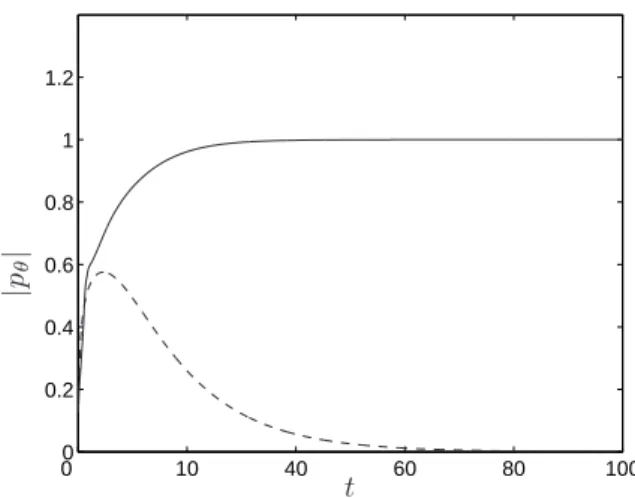
We conclude that synchronization on the circle can be achieved with a local information algorithm whose exchanged information is not only the relative phase but also the estimate of a vector that serves as a consensus reference direction. The global convergence analysis obtained in this way is in contrast with the local convergence analysis proposed in [8,3], for the algorithms (11) and (12). The numerical simulation in Fig.2 illustrates a situation where the (dynamic) local information algorithm (13) achieves synchronization while the (static) algorithm (11) fails to converge. In this example, the communication is a fixed ring topology and the initial phase distribution spreads over more than half a circle. The static algorithm (11) converges to a balanced state where pθ = 0, which is a local minimum of the potential 12 < eiθ, L eiθ >.
6 Global balancing on the N-Torus: dynamic algorithms
Balanced states coincide with the global minima of the cost function V = N
0 0 10 40 60 80 100 0.2 0.4 0.6 0.8 1 1.2 |p θ | t
Fig. 2. Comparison of the behavior of the synchronization parameter |pθ| for two
different local information algorithms when the initial conditions spread over the en-tire circle: the (dynamic) algorithm (15)(full line); the (static) algorithm (11) (dash line). Only the first algorithm achieves synchronization. The simulation involves
N = 20 particles with a random initial condition.
previous section, we now seek to replace the (global information) gradient al-gorithm with a local one. To this end, we consider the continuous-time system
˙θk = − < rk, i >, ˙rk = −i(rk− 1) ˙θk− PN j=1Lkj(t) rjeiθjk, (19)
where rk(0) = 1, ∀ k ∈ I, and its discrete-time version
∆θk[t+1] = arg ³ (1 − δk) − δkrk[t + 1]ei∆θk[t+1] ´ rk[t + 1] = 1 + ³ rk[t] − 1 − ε[t] PN j=1Lkj[t]rj[t] eiθjk[t] ´ e−i∆θk[t+1], (20)
where rk(0) = 1, ∀ k ∈ I, and ε ∈ (0,dmax1 ), dmax= maxk∈Idink.
Theorem 4 Suppose that the communication graph G(t) is uniformly nected and balanced for all t ≥ 0 and that L(t) is bounded and piecewise con-tinuous. Then all the solutions of the decentralized algorithms (19) and (20) asymptotically converge to an equilibrium. Moreover, the only stable limit set is the set of balanced states characterized by pθ = 0. ¤
Proof: (continuous time) Set xk = rkeiθk. The solution x(t) satisfies the
dy-namics
˙x = −L(t)x + d dte
iθ. (21)
The Lyapunov function
W (x) = 1
2 < x, x >,
is not increasing along the solutions of (19): note that, since the graph is balanced, L(t) is a positive semi-definite matrix [19] and then
˙ W = − < L(t)x, x > − N X k=1 < xk, ieiθk >2= − < L(t)x, x > − N X k=1 ˙θ2 k ≤ 0. (22) We deduce from (22) that ˙θ is a function in L2(0, ∞) since (22) implies that
lim t→∞ Z t 0 N X k=1 ˙θ2 k(τ )dτ = W (x(0))−limt→∞ µ W (x(t)) − Z t 0 < L(τ )x(τ ), x(τ ) > dτ ¶ ≤ N 2 .
We deduce from (22) that ˙θ is a function in L2(0, ∞) and that x is uniformly
bounded. To prove that ˙θ asymptotically converges to zero observe that ¨
θk=< Lk(t) x, ieiθk > +(< xk, eiθk > −1) ˙θk
is uniformly bounded, which implies that ˙θ is Lipschitz continuous. We con-clude that ˙θ is uniformly continuous. Then ˙θ is a uniformly continuous function in L2(0, ∞) and from Barbalat’s Lemma we obtain that ˙θ → 0 as t → ∞ [20].
Thanks to the balancing assumption on the graph, 1 is a left eigenvector of L(t), and we obtain from (21) that
1 N < 1, ˙x >= 1 N < 1, d dte iθ > . (23)
Integrating both sides of (23), and using the fact that xk(0) = eiθk(0), one
concludes that 1
N
P
i∈Ixi(t) = pθ for all t ≥ 0. Because x(t) converges to a
consensus equilibrium, each component xk must asymptotically converge to
pθ. As a consequence, the dynamics ˙θk = − < rk, i > asymptotically converge
to the time-invariant dynamics
˙θk= − < pθ, ieiθk >, ∀ k ∈ I. (24)
Since ˙θ is asymptotically convergent to zero, the solutions asymptotically verge to a set of equilibria of (24). We conclude that θ(t) asymptotically con-verges to the critical set of V and, form Theorem 1, that only the set of balanced states is asymptotically stable.
(discrete time) Set xk = rkeiθk. The solution x[t] satisfies the dynamics
x[t + 1] = x[t] − ε[t]L[t]x[t] + eiθk[t+1]− eiθk[t]. (25) As in continuous-time consider the Lyapunov function W (x) = 1
2 < x, x >.
First, we note that, because (I − εL[t]) is a doubly stochastic matrix [2], then kI − ε[t]L[t]x[t]k2 ≤ kx[t]k2
so that
W (x[t + 1]) − W (x[t]) ≤ kx[t + 1]k2− kI − ε[t]L[t]x[t]k2. (26) Next, we observe that
kx[t + 1]k2− kI − ε[t]L[t])x[t]k2
=< x[t + 1], eiθ[t+1]− eiθ[t] > + < eiθ[t+1]− eiθ[t], (I − ε[t]L[t])x[t] > = 2 < x[t + 1], eiθ[t+1] − eiθ[t] > −keiθ[t+1] − eiθ[t]k2
≤ −keiθ[t+1]− eiθ[t]k2, (27)
where the last inequality uses the property that, by definition of θk[t + 1],
< xk[t + 1], eiθk[t+1] >≤< xk[t + 1], eiθk[t] >,
for every k. Using (26) and (27) and summing over t yields
∞
X
t=0
keiθ[t+1]− eiθ[t]k2 ≤ W (x[0]).
The rest of the proof follows from the argument used in continuous-time. ¥ It is worth noting that in contrast to the algorithms (15) and (16), algorithms (19) and (20) are coupled; moreover, this coupling leads (in the discrete-time version) to implicit update equations through the presence of rk[t + 1] in the
nonlinear update equation for θk.
Theorems 3 and 4 generalize the global convergence results of the all-to-all gradient control (4) and (6) under mild assumptions on the communication graph. This generalization is obtained at the prize of increased communication between the communicating agents. They must communicate not only their relative configuration variables θjk but also their estimates rk and rj. In both
theorems, the variable rk can be interpreted as a local estimate of pθ in the
local frame attached to particle k while xk is the local estimate in the absolute
(reference) frame. In design applications, it might be meaningful to exchange additional information between communicating agents in order to relax the cost of global communication architectures.
7 Conclusion
In this paper a novel algorithm is proposed for synchronization and balancing in phase models on the N-torus. In the spirit of earlier work on phase synchro-nization [4], we view synchrosynchro-nization as the task of maximizing the norm of the centroid and balancing as the task of minimizing the norm of the centroid. Gradient-based algorithms require global information because the update law of each agent requires the centroid information. In the proposed algorithm, this global information is estimated on the basis of locally available information, in such a way that the global convergence properties of the original algorithm are asymptotically recovered by the new one. The global convergence analy-sis on the N-torus is a distinctive feature of the present work with respect to previous convergence results that have focused on decentralized consensus algorithms in the Euclidean space. The proposed approach extends beyond phase models on the N-torus. In particular, it can be used to extend in a local information framework global information algorithms proposed in [12], see [13].
References
[1] V. D. Blondel, J. M. Hendrickx, A. Olshevsky, and J. N. Tsitsiklis, “Convergence in multiagent coordination, consensus, and flocking,” in Proceedings of the 44th
IEEE Conference on Decision and Control and European Control Conference,
Seville, Spain, 2005, pp. 2996–3000.
[2] A. Jadbabaie, J. Lin, and S. Morse, “Coordination of groups of mobile autonomous agents using nearest neighbor rules,” IEEE Trans. on Automatic
Control, vol. 48, pp. 988–1001, 2003.
model of coupled nonlinear oscillators,” in Proceedings of the 42nd IEEE
American Control Conference, Boston, Ma, 2004, pp. 4296–4301.
[4] Y. Kuramoto, Chemical oscillations, waves and turbulence. Springer-Verlag, 1984.
[5] N. Leonard, D. Paley, F. Lekien, D. Frantoni, R. Sepulchre, and R. Davis, “Collective motion, sensor networs and ocean sampling,” Proceedings of the
IEEE, 2006, to appear.
[6] W. Li and C. G. Cassandras, “Distributed cooperative coverage control of sensor networks,” in Proceedings of the 44th IEEE Conference on Decision and Control
and European Control Conference, Seville, Spain, 2005, pp. 2542–2547.
[7] L. Moreau, “Stability of continuous-time distributed consensus algorithms,” in
Proceedings of the 43rd IEEE Conference on Decision and Control, Atlantis,
Paradise Island, Bahamas, 2004, pp. 3998–4003.
[8] ——, “Stability of multi-agent systems with time-dependent communication links,” IEEE Trans. on Automatic Control, vol. 50, pp. 169–182, 2005.
[9] R. Olfati-Saber and R. Murray, “Consensus problems in networks of agents with switching topology and time-delays,” IEEE Trans. on Automatic Control, vol. 49, pp. 1520–1533, 2004.
[10]A. Sarlette, R. Sepulchre, and N. Leonard, “Discrete-time syncronization on the
N -torus,” in Proceedings of the 17th International Symposium on Mathematical Theory of Networks and Systems, Kyoto, Japan, 2006, pp. 2408–2411.
[11]L. Scardovi and R. Sepulchre, “Collective optimization over average quantities,” in Proceedings of the 45th IEEE Conference on Decision and Control, San Diego, Ca, 2006, to appear.
[12]R. Sepulchre, D. Paley, and N. Leonard, “Stabilization of planar collective motion with all-to-all communication,” accepted for pubblication in IEEE
Trans. on Automatic Control.
[13]——, “Stabilization of planar collective motion with limited communication,”
IEEE Trans. on Automatic Control, 2006, submitted.
[14]——, “Group coordination and cooperative control of steered particles in the plane,” in Group Coordination and Cooperative Control, (K. Y. Pettersen, J. Gravdahl, H. Nijmeijer (Eds.)), Lecture Notes in Control and Information Sciences, vol. 336, Springer, pp. 217–232, 2006.
[15]S. H. Strogatz, “From Kuramoto to Crawford: exploring the onset of synchronization in populations of coupled oscillators,” Physica D, vol. 143, pp. 1–20, 2000.
[16]——, Sync: The Emerging Science of Spontaneous Order. New York: Hyperion Press, 2003.
[17]T. Vicsek, A. Czirok, E. Ben-jacob, I. Cohen, and O. Shochet, “Novel type of phase transition in a system of self-driven particles,” Physical Review Letters, vol. 75, pp. 1226–1229, 1995.
[18]K. Mischaikow, H. Smith, and H. Thieme, “Asymptotically autonomous semiflows; chain recurrence and Lyapunov functions,” Trans. of the American
Mathematical Society, vol. 347, pp. 1669-1685, 1995.
[19]J. C. Willems, “Lyapunov functions for diagonally dominant systems,”
Automatica J. IFAC, vol. 12, pp. 519–523, 1976. [20]H. K. Khalil, Nonlinear Systems. Prentice Hall, 2001.
![Fig. 1. Interpretation of (6) as a projection onto the manifold S 1 (P , (1 − δ k )e iθ k [t] + δ k p θ [t])](https://thumb-eu.123doks.com/thumbv2/123doknet/5967579.147836/5.892.142.732.328.738/fig-interpretation-projection-manifold-s-p-δ-iθ.webp)