TOWARDS STATION-LEVEL DEMAND PREDICTION FOR EFFECTIVE REBALANCING IN BIKE-SHARING SYSTEMS
PIERRE HULOT
DÉPARTEMENT DE GÉNIE INFORMATIQUE ET GÉNIE LOGICIEL ÉCOLE POLYTECHNIQUE DE MONTRÉAL
MÉMOIRE PRÉSENTÉ EN VUE DE L’OBTENTION DU DILPLÔME DE MAÎTRISE ÈS SCIENCES APPLIQUÉES
(GÉNIE INFORMATIQUE) MAI 2018
c
ÉCOLE POLYTECHNIQUE DE MONTRÉAL
Ce mémoire intitulé :
TOWARDS STATION-LEVEL DEMAND PREDICTION FOR EFFECTIVE REBALANCING IN BIKE-SHARING SYSTEMS
présenté par : HULOT Pierre
en vue de l’obtention du diplôme de : Maîtrise ès sciences appliquées a été dûment accepté par le jury d’examen constitué de :
M. BILODEAU Guillaume-Alexandre, Ph. D., président M. ALOISE Daniel, Ph. D., membre et directeur de recherche
M. JENA Sanjay Dominik, Ph. D., membre et codirecteur de recherche M. LODI Andrea, Ph. D., membre et codirecteur de recherche
ACKNOWLEDGEMENTS
I would especially like to thank my research director Professor Daniel Aloise and my co-director Sanjay Dominik Jena for guiding me and supporting me throughout my master’s degree, and for helping me to target my work.
I also thank Bixi, by the people of Nicolas Blain and Antoine Giraud, for quickly providing me the data and for following the project with interest.
I would also like to thank the chair of "data science for real-time decision making", and especially Andrea Lodi, who funded this project. I also thank the partners of the Chair : GERAD, IVADO and CIRRELT.
I would also like to thank the postdocs, PhD students and masters of the chair who have been assisting me throughout this work and helping me solve my problems.
Finally, I thank the Department of Génie Informatique et Génie Logiciel (GIGL) of Poly-technique Montreal
RÉSUMÉ
Les systèmes de vélos en libre-service sont utilisés à l’échelle mondiale pour soulager la conges-tion et apporter une soluconges-tion aux problèmes environnementaux dans les villes. De nos jours, presque toutes les grandes villes ont un tel système. Ces systèmes sont très pratiques pour les utilisateurs qui n’ont pas besoin de faire l’entretien du vélo et peuvent le rendre presque par-tout dans la ville. Cependant, le nombre croissant d’abonnés et la demande aléatoire rendent la planification opérationnelle du système très difficile. Prédire la demande en vélos a été l’objet de nombreuses recherches dans la communauté scientifique. Cependant, la plupart des travaux ont cherché à prédire la demande globale du réseau, qui n’est généralement pas suffisante pour améliorer la planification opérationnelle. En effet elle nécessite des prévisions spécifiques pour chaque station et à des moments précis de la journée. Ces travaux ont mon-tré qu’une variation significative du trafic peut être liée à des comportements réguliers, et à des facteurs externes tels que les heures de pointe ou les conditions météorologiques. En particulier, de nombreux opérateurs utilisent des intervalles pour combler les lacunes dans la prédiction du trafic. Cependant, très peu de travaux ont cherché à correctement définir ces intervalles.
Dans cette recherche, nous nous concentrons sur la modélisation de la distribution statistique du nombre de déplacements qui se produisent à chaque heure et chaque station. Ce modèle ne se contente pas de prédire l’espérance du nombre de voyages prévus, mais aussi la probabilité de chaque nombre de départs et d’arrivées par station en utilisant la demande historique. Le modèle mis en place est composé de trois parties. Tout d’abord, nous estimons, en utilisant des techniques d’apprentissage machine, le nombre de trajets attendus à chaque station. Puis, nous calculons la confiance sur la première prédiction (variance attendue). Enfin, nous déterminons la bonne distribution à utiliser.
La première partie (espérance du nombre de voyages) utilise un algorithme en deux étapes qui d’abord réduit le problème à un problème plus simple, minimisant la perte d’information, puis un algorithme prédictif est appris sur le problème réduit. Le processus de prédiction de la demande (utilisation du modèle) inverse ce mécanisme. Plusieurs méthodes de simplifica-tion et de prédicsimplifica-tion sont testées et comparées en termes de précision et de temps de calcul (RMSE, MAE, erreur proportionelle, R2, vraisemblance). Les résultats montrent que le choix du meilleur algorithme dépend de la station. Un modèle combinant les modèles précédents est proposé. Ces algorithmes utilisent la demande des stations voisines pour améliorer leurs per-formances en les agrégeant. Ils extraient des stations des comportements principaux qui sont
ensuite modélisés. Ces comportements sont alors plus simples et stables (moins aléatoires). Les conclusions de ce travail sont validées sur les réseaux de Montréal, New York et Washing-ton. Enfin, ce modèle est utilisé pour définir une stratégie de rééquilibrage en temps réel pour Bixi à Montréal, en raffinant la définition des intervalles de rebalancement.
ABSTRACT
Bikesharing systems are globally used and provide relief to congestion and environmental issues in cities. Nowadays, almost all big cities have a bicycle-sharing system. These systems are very convenient for users that don’t need to do maintenance of the bicycle and can return it almost everywhere in the city. However, the increasing number of subscribers and the sto-chastic demand makes the operational planning of the system very difficult. Predicting bike demand has been a major effort in the scientific community. However, most of the efforts have been focused on the prediction of the global demand for the entire system. This is typically not sufficient to improve the operational planning, which requires demand predictions for each station and at specific moments during the day. A significant variation of the traffic can be linked to regular behaviors, and external factors as peak hours or weather. In particular, many system operators use fill level intervals which guide the redeployment crews in their efforts to equilibrate the system. However, little work has been done on how to effectively define those fill levels.
In this research, we focus on modeling the distribution of the number of trips that occur at each hour and each station. This model not only seeks to predict the number of expected trips, but also determines as precisely as possible the expected distribution of trips. It uses the historical observed demand to predict future demand. The prediction model is composed of three parts. First, we estimate from historical data the expected number of trips, using ma-chine learning techniques that use features related to weather and time. Second, we compute the confidence of the first prediction (expected variance). Finally, we focus on determining the right distribution to use. The first part uses a two-step algorithm that first reduces the problem to a simpler one, minimizing the information lost, then learns a predictive algorithm on the reduced problem. The prediction process inverts this mechanism. Several simplifica-tion and predicsimplifica-tion methods are tested and compared in terms of precision and computing times. The final test compares distribution estimations in terms of log likelihood. The re-sults show that the choice of the best algorithm depends on the station. Then a combined model is proposed to better model the demand. Our models are tested on several networks (Montreal, New York and Washington). Finally, this model is used to define an online reba-lancing strategy close to the one used by Bixi at Montreal. This strategy has been deployed in Montreal.
TABLE OF CONTENTS
ACKNOWLEDGEMENTS . . . iii
RÉSUMÉ . . . iv
ABSTRACT . . . vi
TABLE OF CONTENTS . . . vii
LIST OF TABLES . . . x
LIST OF FIGURES . . . xi
LIST OF ACRONYMS AND ABBREVIATIONS . . . xiii
LIST OF APPENDICES . . . xiv
CHAPTER 1 INTRODUCTION . . . 1
CHAPTER 2 LITERATURE REVIEW . . . 5
2.1 Classification of problems in bike-sharing systems . . . 5
2.2 First Level : Network Design . . . 5
2.3 Second level : Traffic analysis . . . 7
2.4 Second Level : Estimating Lost Demand . . . 10
2.5 Third level : Redistribution . . . 10
2.6 Third Level : Targets for Rebalancing . . . 12
2.7 Summary . . . 12
CHAPTER 3 DATA ANALYSIS . . . 16
3.1 Bixi’s Data . . . 16
3.1.1 Bixi private data . . . 18
3.2 Weather data . . . 19
3.3 Holidays and National Days . . . 20
3.4 Preprocessing . . . 20
3.4.1 Features preprocessing . . . 20
3.4.2 Objective preprocessing . . . 21
3.6 Feature Analysis . . . 23
3.6.1 Feature significance . . . 28
3.6.2 Data analysis conclusions . . . 29
CHAPTER 4 MODELING DEMAND PER STATION . . . 30
4.1 General Overview . . . 30 4.2 Evaluating models . . . 32 4.2.1 Splitting Data . . . 33 4.2.2 Size of Stations . . . 33 4.2.3 MAE . . . 33 4.2.4 RMSE . . . 34 4.2.5 MAPE . . . 34 4.2.6 RMSLE . . . 34 4.2.7 R2 Score . . . . 34
4.3 Predicting Traffic Expectation . . . 36
4.3.1 Literature . . . 38
4.3.2 Reduction Methods . . . 38
4.3.3 Reconstruction loss and reduction optimization . . . 43
4.3.4 Prediction Methods . . . 48
4.4 Expectation Hyperparameters Optimization . . . 51
4.4.1 Selection of the number of dimension, optimization of reduction methods 51 4.4.2 Linear Regression . . . 52
4.4.3 Decision Tree . . . 53
4.4.4 Random Forest . . . 53
4.4.5 Gradient Boosted Tree . . . 54
4.4.6 Multi-Layer Perceptron (MLP) . . . 54
4.5 Test of mean traffic estimation model . . . 55
4.5.1 Test of Data Transformations . . . 55
4.5.2 Features importance analysis . . . 62
4.5.3 Analysis of the results of the proposed algorithms . . . 64
4.5.4 Ensemble Model for mean estimation . . . 65
4.6 Predicting Traffic Variance . . . 69
4.6.1 Variance hyperparameters optimization . . . 71
4.6.2 Variance estimation results . . . 73
4.7 Fitting the Trip Distribution . . . 74
4.7.2 Poisson Distribution . . . 75
4.7.3 Negative Binomial Distribution . . . 76
4.7.4 Zero Inflated Poisson . . . 76
4.7.5 Distribution Results . . . 77
4.8 Results on the Test dataset . . . 80
4.8.1 General Results . . . 80
4.8.2 Results per stations : stations 6507, 5005, 6221 . . . 84
4.8.3 Geographical distribution . . . 87
4.8.4 Adding new stations . . . 89
4.9 Application on other bike-sharing networks . . . 89
4.9.1 Montreal . . . 89
4.9.2 Washington . . . 90
4.9.3 New York . . . 91
4.9.4 Conclusions . . . 91
CHAPTER 5 GENERATING DECISION INTERVALS FOR REBALANCING . . 93
5.1 Service Level . . . 93
5.1.1 Modification of the service level . . . 94
5.1.2 Time Horizon . . . 95
5.1.3 Implementation Notes . . . 95
5.1.4 Analysis of the Service Level . . . 95
5.2 Defining decision intervals . . . 96
5.2.1 Test of decision intervals . . . 98
5.2.2 Results on the decision intervals . . . 100
5.2.3 Estimating the marginal improvement of increasing the rebalancing capacity . . . 103
CHAPTER 6 GENERAL DISCUSSION . . . 106
CHAPTER 7 CONCLUSION . . . 110
REFERENCES . . . 113
LIST OF TABLES
Table 2.1 Contribution in bike-sharing system rebalancing . . . 13
Table 2.2 Main contribution is traffic modeling . . . 14
Table 3.1 Missing data numbers . . . 22
Table 3.2 gap occurrences . . . 23
Table 3.3 Available features for the model . . . 23
Table 3.4 Selected features for the model . . . 29
Table 4.1 Summary of principal characteristics of reduction methods . . . 47
Table 4.2 correlations between RM SE score of four different algorithms, varying the random forest hyperparameters. . . 51
Table 4.3 Precision of the log transformation compared to the normal data . . . 56
Table 4.4 Impact of the decorrelation on the precision . . . 56
Table 4.5 Impact of the normalization on the precision . . . 57
Table 4.6 average performance of time augmented models . . . 60
Table 4.7 Precision and running time of mean estimators . . . 64
Table 4.8 Comparison of reduction methods, using a linear predictor . . . 65
Table 4.9 Results of combined algorithms . . . 68
Table 4.10 Performance of estimators on variance after optimization . . . 72
Table 4.11 Precision of variance estimators (validation set) . . . 73
Table 4.12 Average Log likelihood per distribution hypothesis of several models . 78 Table 4.13 Proportion of votes per hypothesis . . . 78
Table 4.14 scores of each model on the test set . . . 83
Table 4.15 Scores on three stations . . . 85
Table 4.16 Scores on Montreal (Bixi) without weather features . . . 90
Table 4.17 Scores on Washington (Capital Bikeshare) . . . 90
Table 4.18 Scores on CityBike (New York) . . . 91
Table 5.1 average sum of minimums, targets and maximums per hour . . . 99
Table 5.2 Decision interval scores . . . 102
Table 5.3 Influence of α value . . . . 104
Table A.1 Precision scores for mean estimation algorithms on validation set . . 119
Table B.1 Scores on Montreal (Bixi) without weather features . . . 123
Table B.2 Scores on Washington (Capital Bikeshare) . . . 124
LIST OF FIGURES
Figure 3.1 Example of a trip file . . . 17
Figure 3.2 Example of precipitation file . . . 19
Figure 3.3 Repartition of traffic during the week (Monday to Sunday) . . . 21
Figure 3.4 Trip Numbers per Feature . . . 26
Figure 3.5 Correlation matrix . . . 27
Figure 3.6 ANOVA results . . . 28
Figure 4.1 Model preview . . . 31
Figure 4.2 Model for mean prediction . . . 36
Figure 4.3 Explained variance ratio per singular value . . . 44
Figure 4.4 SVD first components . . . 45
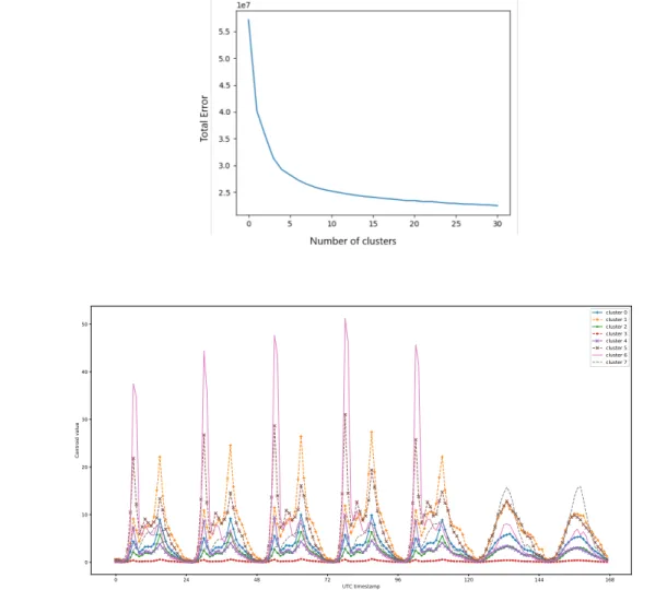
Figure 4.5 Kmeans analysis . . . 46
Figure 4.6 RM SE per dimension for kmeans and SVD . . . . 52
Figure 4.7 Scores evolution per time window . . . 58
Figure 4.8 First time dependent model . . . 59
Figure 4.9 Second time dependent model . . . 59
Figure 4.10 R2 score during the jazz week (first figure) and a September week (second figure), for hours between 2h p.m. and 2h a.m. . . 61
Figure 4.11 Feature importance for decision tree algorithms . . . 63
Figure 4.12 Number of stations for which each algorithms is the best . . . 66
Figure 4.13 Medium size of stations per best algorithm . . . 67
Figure 4.14 Votes for algorithms (orange first vote, blue second vote) . . . 68
Figure 4.15 Residuals versus features . . . 70
Figure 4.16 Votes for best algorithms, based on the best RM SE . . . 79
Figure 4.17 Error Deviation . . . 82
Figure 4.18 Station size versus MAPE . . . 84
Figure 4.19 Station size versus R2 . . . 85
Figure 4.20 Predicted and real Traffic in station 6221 . . . 86
Figure 4.21 Predicted and real Traffic in station 6307 . . . 87
Figure 4.22 Predicted and real Traffic in station 5005 . . . 88
Figure 4.23 Geographical distribution of the error . . . 88
Figure 4.24 Station sizes per network . . . 92
Figure 5.1 Evolution of the service level with different time horizons, from 2 hours (gray) to 100 hours (black) . . . 96
Figure 5.2 Selection of station’s service level in the same period . . . 96
Figure 5.3 Rules to compute decision intervals on station 46 and 202 . . . 98
Figure 5.4 Evolution of scores in respect to β (α = 0.5) . . . . 102
Figure 5.5 Evolution of scores in respect to α (β = 0.65) . . . 103
Figure 5.6 Marginal utility of rebalancing . . . 104
Figure 5.7 Distribution of rebalancing operation during the day . . . 105
Figure 7.1 Adaptive model flowsheet, on the top left box the learning of the pre-dictive algorithm, on the top right box the learning of the adaptive part and the bottom the global prediction process . . . 111
LIST OF ACRONYMS AND ABBREVIATIONS
RL Reconstruction Loss
RLnorm Normalized Reconstruction Loss
M AP E Mean Absolute Percentage Error RM SE Root Mean Squared Error
RM SLE Root Mean Squared Logarithmic Error M AE Mean Absolute Error
R2 Coefficient of determination ANOVA ANalysis Of Variance
arr arrival
dep departure
SVD Singular value decomposition GM Gaussian Mixture
id Identity
GBT Gradient Boosted Tree DT Decision Tree
AE AutoEncoder
RF Random Forest
LIST OF APPENDICES
Annexe A PRECISION RESULTS . . . 119 Annexe B RESULTS ON MONTREAL, WASHINGTON AND NEW YORK . . 123
CHAPTER 1 INTRODUCTION
Bikesharing systems are widely used and offer an appropriate solution to congestion in big cities. Today almost all big cities have their own bikesharing system. Three generations of systems led to an efficient and reliable one, which does not suffer from thefts and deterioration. These systems are very convenient for users that don’t need to do the maintenance of the bicycle and can return it almost everywhere in the city. However, the increasing number of subscribers and variability of the demand makes the operation and maintenance of the system very hard.
In this context, traffic prediction and network rebalancing are the main operational goals of the system operator. The operator’s role is to ensure that it is always possible to rent or return a bicycle in every station. However, people behavior is variable and hard to predict. The operator also needs to consider the natural trend of the network to unbalance. These two difficulties are worsened by the difference in response times. While it takes less than one hour for the network to unbalance, the operator needs more than half a day to visit all stations once. Thus, the operator needs to anticipate three to six hours before the evolution of the system, to be able to prepare it. Therefore the operator is interested into modeling the traffic using exogenous factors as the time and the weather.
Some work has been done to optimize rebalancing strategies but failed to provide a solution applicable by the industry. Besides, today traffic prediction is mostly done using empirical prediction and operators experience. Thus, rebalancing is performed using greedy strategies based on the empirical targets. Traffic has been analyzed from a global point of view, but the literature on traffic prediction per station is rare.
This work explores several traffic models and selects the more precise and efficient one. It studies the dependencies between the bike traffic and some exogenous features as time and weather. This work also proposes an online rebalancing strategy that uses the traffic model to improve the service level of the operator. This strategy is inspired from the operator’s one and is directly applicable to real world problems.
Bixi Montreal
This work has been done in partnership with Bixi Montreal, the operator of the Montreal system. This section presents the environment and challenges of this project. Bixi is a network of 5220 bicycles and 462 stations (2016). It has been created by order of the city of Montreal,
and has been inspired by similar models, in European cities. The initiative was part of the transportation plan "reinventer Montreal" of 2008. PBSC took the responsibility of developing and deploying the network. They used the technology already used for parking slots. Bixi is a relatively big network. It began in 2009 with 3000 bicycles and 300 stations, deployed mainly in downtown and in the densely populated areas. 160 stations and 2000 bicycles were added in 2010 to complete the system and to reach the 2016 one. In 2017 Bixi expanded its network to achieve 6000 bicycles and 540 stations. This work is based on the 2016 network. Bixi is part of the third generation of bikesharing systems. The first generation used free bicycles painted in a specific color that anybody could rent and return, but due to technical limitations (theft and deterioration), these systems were closed or updated. The second-generation systems introduced docks and money deposits to rent bicycles. Bicycles were also designed to resist to vandalism. However, these systems are more expensive than the first one, and are financed by municipalities. Though thefts continued, and the service level dropped, the third generation introduced limited time rent and used wireless technology to follow in real time the evolution of the network, considerably improving the service level.
Bixi has 35 000 members and 235 000 users that make 4 million trips each year, using 5 to 6 times each bicycle a day. Then rebalancing optimization is a priority for the operator. Bixi uses 10 trucks of a capacity of 40 bicycles to counter the unbalance generated by users. They are able to tracks in real time the network status using wireless (solar powered and wireless communication) and movable stations of variable capacity. Montreal traffic is also limited by the weather, during winter it snows about 200 cm in total. The network is then closed between November and April.
Bixi deployment was very successful and their system was exported to other cities as London (687 stations), Minneapolis (146), Washington (252), New York (600) and Chicago (400). The system is also used in Ottawa (25), Melbourne (52), Toronto (80), Boston (90), Chattanooga (30) and Pittsburgh (50).
Bixi challenge today is to assure the best service level for their users, optimizing their re-balancing operations. For that purpose, it uses a handmade decision process for rere-balancing based on acceptable fill levels.
Objectives
This work seeks to model as accurately as possible the bicycle traffic in Montreal. It also provides a methodology and conclusions applicable to other cities. The model tries to define the influence of a maximum of features on the bikesharing traffic. These features are mainly time or weather-related. The model is also built to predict the probability distribution of the number of trips per station, and not only its expectation. To accomplish this goal, this work seeks to show the pertinence of a problem reduction approach that is able to take advantage of station similarities, while being specific to each station.
This work also seeks to propose an application of the model in a real situation. This work uses the model to improve the operator rebalancing strategy by optimizing station inventory. This work is also intended as a preliminary to a reinforcement learning approach of network rebalancing problem.
Work Overview
This dissertation presents all the work done to build the proposed traffic models and their application to real world problems, as well as its deployment into the Bixi system. This work covers the subject in the following way.
The first chapter presents a literature review that covers most articles about traffic analysis in bikesharing systems. A quick overview of the work done in rebalancing is done to justify the need for accurate traffic prediction. Papers on traffic analysis are classified from their objectives in traffic design and traffic prediction. A gap in traffic prediction is shown, and this work proposes a methodology to fill it. The second chapter presents the available data from Bixi, Citybike, Capital Bikeshare and Données Canada. It presents trip data, weather data, critical event data and station data for each bikesharing system. This data is analyzed to extract the relevant information and transformed to suit the problem requirements. All preprocessing steps are described.
The third chapter presents the proposed model for traffic modelization per station and per hour. This chapter is divided into five sections. The first section presents the architecture and the methodology used to build the model : a two-phased algorithm with a simplification part and a prediction part. The second section presents the first step of the methodology : predicting the traffic expectation. A new method is proposed for multiple prediction, using a simplification of the problem extracting main behavior and predict station traffic from these behaviors. The next section analyzes and predicts traffic variance, by performing a new feature
selection. The fourth section uses the first two predictions (expectation and variance) to fit a statistical distribution on the model (on each station). This section completes the model. The last section compares different algorithms built by this methodology and compare them to state-of-the-art algorithms. All algorithms are compared in terms of precision, rapidity and likelihood.
The fourth chapter presents an application of the model to a real-world problem by auto-mating intervals and target generations. This application improves the performance of Bixi’s strategy, giving a mathematical background to the decision intervals used to rebalance the system. These intervals are generated using this probabilistic model and service level. The generated intervals are tested on real data using a worst-case approach. They are compared to Bixi ones.
Finally, the dissertation concludes on the best methods to predict bikesharing traffic expec-tation, and proposes future work based on these models.
CHAPTER 2 LITERATURE REVIEW
2.1 Classification of problems in bike-sharing systems
A lot of problems are related to bike-sharing systems, the main and most addressed one in the literature is the management of the demand. The main issue with the demand is to address it at every time of the day, every day. The system has a natural trend to unbalance itself because most travels are short and one way (Vogel and Mattfeld, 2010). They also study the traveling causes and identify two main sources of unbalance : continuous sources and discrete sources. Examples of continuous sources are the height difference and peak hours. Discrete sources are for example weather, events, underground failures, which are unpredictable or irregular. The system operator goal is to counter this unbalance to meet the demand by means of very limited resources.
The operator has three decision levels : the first, the long-term level, is used for the design of a new network or an expansion or modification of an existing one. On this level, the aim is to place stations and evaluate potential demand analyzing neighboring effects. The second level is a mid-term level in which the operator fixes hourly objectives based on historical behavior of the system. The fixed objectives can be set every month but also in real time. This part uses knowledge about the network to influence operator behavior. The last level is the operational level, the online level. The operator takes real-time decisions on the network to balance it and uses the analysis and results of the second to better serve the demand. The problems tackled in each level are :
— First level corresponds to the network design
— Second level rebalancing planning, demand modelization — Third level rebalancing operations, network maintain
This work proposes a traffic prediction tools (second level). However, the built model uses weather transforming the model into a real-time prediction model, getting it closer to a third-level decision.
2.2 First Level : Network Design
The first level of decision is the network design. This level tries to define the area to be covered, the number of locations and size of stations, the number of bicycles, and evaluates the repositioning possibilities. This problem is very close to the demand prediction problem : the main goal is to explain the demand using external factors, as weather, time, but also
environment (connections, or neighboring activity). Traffic modelization and network design share the same goal : they try to explain the demand from exterior factors. However, the analyzed features are different, the network design problem is more interested in how neigh-boring activity will influence the demand, whereas in traffic modelization these effects are contained into the station behavior and are static. Then neighboring effects are ignored most of the time for traffic prediction. Only models that aim to handle breakdowns and rare effects take these effects into consideration.
A lot of articles tried to explain the demand from neighboring properties. Mahmoud et al. analyze the effect of socio-demographic attributes, land use, built environment and some weather measures. They show an effect on the distance between stations and the number of neighboring intersections. Faghih-Imani and Eluru (2016) also analyze these effects, and prove a dependence with surrounding restaurants, parks, bike lanes and job and population density. Rudloff and Lackner (2014) in a similar analysis shows that the traffic depends on the neighboring station status, and weather conditions (temperature, humidity, rain). Hampshire and Marla (2012) also analyze the relationship between the bike-sharing traffic and other transportation means. They show that this relationship depends on the hour of the day. Gebhart and Noland (2014) analyze the impact of weather conditions on the bike traffic. Vogel and Mattfeld (2011) analyze the relationship between time and spacial imbalancement due to one-way trips and short rental times. Vogel et al. (2011) uses the time features to forecast bike demand and simulate the evolution of the network. They refine their model using some weather measures (temperature, rainfall, wind and humidity). Etienne and Latifa (2014) model the traffic and cluster stations into work, residential, leisure, and train stations. They also show that the trip count depends on the day of week and the hour of the day. Borgnat et al. (2011) model the time evolution of Lyon’s bike-sharing system using autoregressive methods. This work also analyzes the effect of connections on the user’s behavior.
These works showed that the traffic in the network depends on the distance of the trip (Mahmoud et al.; Faghih-Imani and Eluru, 2016), the vicinity of the station (Mahmoud et al.; Faghih-Imani and Eluru, 2016; Hampshire and Marla, 2012; Etienne and Latifa, 2014), the neighboring stations (Rudloff and Lackner, 2014), the available connections (Faghih-Imani and Eluru, 2016; Hampshire and Marla, 2012; Etienne and Latifa, 2014; Gebhart and Noland, 2014), the weather (Mahmoud et al.; Gebhart and Noland, 2014; Borgnat et al., 2011; Vogel et al., 2011; Vogel and Mattfeld, 2011), the temperature (Mahmoud et al.; Rudloff and Lackner, 2014; Gebhart and Noland, 2014; Vogel et al., 2011; Vogel and Mattfeld, 2011), the day (Faghih-Imani and Eluru, 2016; Hampshire and Marla, 2012; Etienne and Latifa, 2014; Borgnat et al., 2011; Vogel et al., 2011; Vogel and Mattfeld, 2011), the period of the year (Rudloff and Lackner, 2014; Gebhart and Noland, 2014; Borgnat et al., 2011), the number
of bicycles in service (Borgnat et al., 2011; Vogel et al., 2011; Vogel and Mattfeld, 2011; Shu et al., 2010), the number and the size of stations (Faghih-Imani and Eluru, 2016; Borgnat et al., 2011; Shu et al., 2010), the influence of exceptional events (Fanaee-T and Gama, 2014), the labor market (Faghih-Imani and Eluru, 2016; Hampshire and Marla, 2012; Borgnat et al., 2011) and the sociology of the people (Mahmoud et al.; Faghih-Imani and Eluru, 2016; Etienne and Latifa, 2014; Borgnat et al., 2011; Vogel et al., 2011; Vogel and Mattfeld, 2011; Lathia et al., 2012). MEng (2011) proposed a method to estimate the propensity to pay for users. Lin and Yang (2011); García-Palomares et al. (2012); Lin and Chou (2012); Martinez et al. (2012) proposed also some methods to determine the optimal number of stations and their location in terms of the environment of the station, the available infrastructure and the expected demand. These studies show that the demand depends on a lot of factors, however, a few of them are pertinent in the short term forecasting demand.
2.3 Second level : Traffic analysis
Demand modelization is essential to a good redistribution model that bases its decisions on the expected demand. Even if most papers on rebalancing use a simple modelization of the demand, some papers propose more accurate modelizations. However, the stochasticity of the problem is important, and it is not completely predictable. A simpler version of the problem studied by most papers is the modelization of the global demand, i.e. the total number of departures or arrivals in the given period. Papers analyzing the demand focus on two objectives the first is to find and evaluate relations between the demand and some factors, the second tries to predict as accurately as possible the demand. The first papers showed that the demand depends on the hour, the week day, the month, the temperature and the meteorology(Borgnat et al., 2011; Gebhart and Noland, 2014; Mahmoud et al.; Vogel et al., 2011; Vogel and Mattfeld, 2010). They also prove the dependency to humidity, wind speed, night, number of stations, user gender, universities, jobs and neighborhood of the station. Bordagaray et al. (2016) identify five purposes of trips and classifies trips into these five classes : round trips, rental trips reset, bike substitution, perfectly symmetrical mobility trips and non-perfectly symmetrical mobility trips. Borgnat et al. (2011); Gebhart and Noland (2014); Hampshire and Marla (2012); Lathia et al. (2012); Mahmoud et al.; Vogel et al. (2011); Vogel and Mattfeld (2010) propose statistical models for global demand prediction. They achieve a R2 (explained variance) score between 50 and 70%. Other authors focus their work into predicting as accurately as possible the global demand. A Kaggle (kag, 2014) contest took place in 2014-2015 to predict the demand in the Washington network. A RMLSE (root mean logarithmic squared error) score of 0.33 was achieved. The most effective
algorithms were based on a gradient boosted trees (Yin et al., 2012).
Wang (2016) analyzed the traffic of New York and tried to accurately predict the global demand using weather and time features. He analyzed the features and proposed a random forest regressor to complete missing weather data. He also improved significantly its perfor-mance by using a log transformation of the trips counts. Cagliero et al. (2017) build a model to predict critical status of stations using Bayesian classifiers, SVM, decision trees. They use the hour, the day and if it is a working day to predict if a station is critical (full or empty) Rudloff and Lackner (2014) also predict traffic per station and uses neighboring information to refine its prediction. Yin et al. (2012) predicts the global demand on Washington’s network using time and weather features. They show that the prediction problem is highly nonlinear. They used a gradient boosted tree to predict the demand. Li et al. (2015) use a gradient boosted tree to predict the traffic by station, by clustering them geographically. Vogel and Mattfeld (2010); Yoon et al. (2012) used an ARMA (AutoRgressive Moving Average) mo-del for the demand. Some deep learning momo-dels have been proposed (Polson and Sokolov, 2017). These models can compete with the gradient boosted tree but need much more tuning experience to be optimized.
Zhang et al. (2016) analyzed the trip behavior and shown a time dependency of trips. They try to predict the arrival station and time of users, knowing their departure station and time. Most papers use a one-hour time step for prediction, Rudloff and Lackner (2014) prove that this time step is a good balance between time precision and count precision. A lot of different models have been developed to explain and predict bicycle traffic, though only a few articles tried to model the traffic per station, most articles are interested in the global prediction. The traffic prediction par station problem is different from the previous one because the stochasticity is much more present. This stochasticity makes the problem more challenging. A proposed strategy to predict the traffic is to reduce the problem using clustering (group together similar stations) (Li et al., 2015; Vogel et al., 2016; Chen et al., 2016). The clustering can be performed geographically (Li et al., 2015) or only using station behavior (Vogel et al., 2016). The prediction on the clusters are understandable and accurate but the operator usually needs an estimation of traffic per station, and such models can only capture global behaviors. Vogel et al. (2016) propose simple rules to deduce from the traffic estimation between clusters, the traffic between stations. These rules give good insight on the traffic, but constraint stations too much besides underfitting the data.
Some papers also focused their work on predicting the evolution of the network in a short time period : Cagliero et al. (2017) try to predict when stations will be in a critical state. Yoon et al. (2012) build a model that predicts with high accuracy the network status in the
next hour, allowing the user to find available stations.
Rudloff and Lackner (2014) proposed a model for predicting traffic per station. The proposed model tries to predict the traffic per station and per hour using time and weather data. They also use neighboring station status as features for their algorithm. A simple linear regression is performed on the data, using categorical variables for time, weather, season, week day and temperature. Several distributions have been tested on the data and they conclude that the Poisson model is not always the best distribution and that the zero inflated and negative binomial distributions are also well suited for this problem. However, they tested their model only in Vienna’s system, a medium-sized bike sharing system (about 100 stations). Their conclusions could be different on other networks. Proposed distributions increase the probability of zero trips and is then suited for a low activity network. Their study also tried to compute the influence of neighboring critical status on the demand, but they could not establish a clear dependency.
Gast et al. (2015) proposed a model to predict traffic using historical data. They used a queuing model, estimating for each time step the Poisson parameter. They used 15 minutes time steps. They estimated the Poisson parameters naively, taking the average value for all previous days. The authors also showed that the RMSE (Root mean square error) score, and similarly all precision scores are not adapted to stochastic problems, as perfect models do not give zero errors. They introduce new scores to compare models but neglected the log likelihood 4.7. They also compare their work to very naive approaches.
Yoon et al. (2012) propose a model that uses real-time network status to predict its evo-lution in a short horizon of time. They use a similarity approach to simplify the problem. They propose an ARMA (AutoRegressive Moving Average) model that considers neighboring stations, time and meteorology to predict the evolution of the network. The neighborhood is estimated with three different methods : A K-NN (k nearest neighbors) on station patterns, linear regression to predict the return station and a Voronoï approach to define neighboring stations. They achieve similar results with the three proposed station aggregation patterns. Their results are hardly comparable as they use short time RMSE and the precision of the algorithm. They achieve a RMSE score of 3.5 after one hour, i.e. the model is 3.5 trip away from the real value after one hour on average.
Zhou et al. (2018) build a model using Markov’s chain to compute the stable point of the network and infer the out and in flow of each station. They also use weather and time feature to refine their model. However, they only predict the expected daily traffic.
2.4 Second Level : Estimating Lost Demand
The prediction of demand from historical data is intrinsically biased since it covers only sa-tisfied demand. However, part of the demand is not sasa-tisfied, mostly due to critical situations (full or empty) in stations. This part of the demand is most of the time minor compared to the total demand but needs to be considered for the evaluation of prediction and rebalance-ment algorithms. The absence of lost demand estimation, leads to reproduce bad decisions by reproducing the operator’s strategy. Papers proposed several ways to counter this bias, the most common is to use the random generation of trips from a Poisson distribution, whose parameters have been deduced from historical data (Brinkmann et al., 2015; Shu et al., 2010; Alvarez-Valdes et al., 2016). This strategy generates a traffic slightly different from the real one, to prevent overfitting. This bias is ignored in Vogel and Mattfeld (2010); Caggiani and Ottomanelli (2012); Mahmoud et al.; Yin et al. (2012); Schuijbroek et al. (2013). Rudloff and Lackner (2014); Chen et al. (2016) clustered stations to erase lost demand bias. Yoon et al. (2012) used similarity measured between stations to estimate lost demand.
2.5 Third level : Redistribution
The redistribution problem is one of the most addressed problems in the literature about bike sharing. The redistribution operations are meant to be the third level. However the length the time needed to solve the problem makes it more second level : These algorithms can only be used to plan the rebalancing. They cannot be used in real time. The redistribution problem can be cast as an optimization problem : the goal is to maximize the total number of trips, while minimizing the cost of redistribution. The redistribution problem is a pickup and delivery problem Raviv et al. (2013), with a fixed number of trucks and a variable and stochastic demand. The problem needs to track the time steps, the number of trucks, the number of stations and the status of the network. All these components make the problem intractable, and some approximations are necessary to solve the problem. The first approxi-mation is to consider the static problem, which is realistic during the night. The aim of this problem is then to reach some pre-established objectives at each station, while minimizing some measure as the cost of the company or the rebalancing time. Some approximations are also made on the number of trucks, usually reduced to one, with finite or infinite capacity. Chemla (2012) proposes a solution, using two trucks and an infinite amount of time and tries to minimize the traveled distance. Benchimol et al. (2011) proposes a solution with one truck of finite capacity and an infinite time horizon, minimize the company cost. Raviv and Kolka (2013) try to minimize the lost demand, and maximize the service level, a measure
of the expected proportion of satisfied demand. Schuijbroek et al. (2013) use integer pro-gramming and constraint propro-gramming to solve the problem. They also propose a heuristic that performs better than the solution of the integer and constraint programming because of the approximations made in these models. All these formulations have the same scalability problem : they manage to solve the problem to optimality (with some approximations) only for networks with fewer than 100 stations. Some papers also try to solve the dynamic pro-blem. This problem offers the possibility to give incentives to users to do some specific trips (Chemla, 2012; Fricker and Gast, 2013; Waserhole and Jost, 2012). They also conclude that these incentives cannot replace the operator. Chemla (2012) proposes three greedy strategies to rebalance the network and concludes that modeling the demand can considerably improve rebalancing. Contardo et al. (2012) propose a mathematical model to solve the problem, but the scalability issue is not solved, and solutions can be found only on small instances. Lin and Chou (2012); Leduc (2013); Lowalekar et al. (2017) also proposed some formulations of the problem. Lowalekar et al. (2017) uses expected future demand and scenarios, to find efficient repositioning strategies.
All these approaches try to optimize the satisfied demand, and use objectives, intervals, or demand estimation to simulate the demand. The most common strategy is to simulate the demand through a Poisson process (Alvarez-Valdes et al., 2016; Raviv and Kolka, 2013; Vogel et al., 2016; Vogel and Mattfeld, 2010). However, these models most of the time do not consi-der the influence of external factors. The Poisson hypothesis is pertinent in most cases as it describes independent arrival and departure on each station. Other articles use given objec-tives to be satisfied (Anily and Hassin, 1992; Benchimol et al., 2011; Berbeglia et al., 2007; Chemla et al., 2013; Hernández-Pérez and Salazar-González, 2004; Leduc, 2013). Usually these objectives are defined by the operator and are used to take rebalancing decision. They are defined, empirically, using historical demand. Schuijbroek et al. (2013) propose intervals based on the service level instead of targets, as objectives. This approach is more complete as it considers the variability of the demand for rebalancing and ensure a minimum service level on the network. This approach is also close to the one used by operators to rebalance the network : they use intervals to decide when to rebalance a given station. Schuijbroek et al. (2013) model the demand through a Markov chain, with some given probability to remove or add a bicycle. The modeled demand is time dependent. Caggiani and Ottomanelli (2012) propose a fuzzy logic algorithm to model the urgency of rebalancing a given station. This method also gives a heuristic to rebalance the network. However, it does not consider the distances.
2.6 Third Level : Targets for Rebalancing
Most rebalancing methods uses fill targets on each station, the same objectives used by the operator to make decisions. However, these objectives should be defined carefully because they are essential to assure a good decision process and should consider several factors such as the future demand. These objectives can be formulated as the expected demand or can have more complex forms. A lot of articles (Alvarez-Valdes et al., 2016; Raviv and Kolka, 2013; Vogel et al., 2016, 2014) suppose that the demand has a Poisson distribution, but ignore the effect of external factors as the weather and the time. Other articles suppose these objectives are given, (Anily and Hassin, 1992; Benchimol et al., 2011; Berbeglia et al., 2007; Chemla et al., 2013; Hernández-Pérez and Salazar-González, 2004; Leduc, 2013). Schuijbroeck is the first to propose intervals and not only objectives and uses them for his rebalancing algorithm. These intervals are also used by Brinkmann et al. (2015) to solve the rebalancing problem and in short and long-term heuristics. Caggiani and Ottomanelli (2012) uses a fuzzy logic algorithm to model the urgency of rebalancing on each station.
2.7 Summary
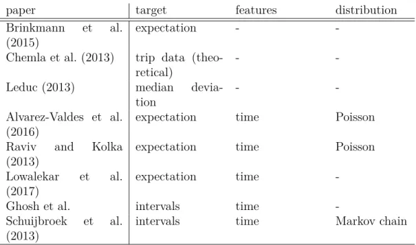
Table 2.1 and 2.2 presents a summary of the main contributions in terms of rebalancing (2.1) and traffic prediction (2.2). For each article it presents how they model each key part of the problem, and what is their objective. Table 2.1 presents some rebalancing papers. Some of these papers predict traffic, and other suppose a distribution of arrivals and departures. The table also tells how the traffic model is used in the work. Table 2.2 presents main works in terms of traffic prediction. It presents which features are used, what is the goal of the paper, which prediction level they use. And gives a quick overview of their prediction method. This work is presented in the last line of this table. The last column presents some scores presented in the papers. In this table, LR stands for linear regression, GBT for gradient boosted tree, SVR for support vector regression, SVM for support vector machine, GLM for generalized linear models, ZI for the zero inflated distribution. The NB acronym is ambiguous, if it is in the distribution column, it stays for Negative binomial. If it is in the prediction column, it stays for Naive Bayes.
Table 2.1 Contribution in bike-sharing system rebalancing
paper target features distribution
Brinkmann et al. (2015)
expectation -
-Chemla et al. (2013) trip data (theo-retical)
-
-Leduc (2013) median devia-tion
-
-Alvarez-Valdes et al. (2016)
expectation time Poisson
Raviv and Kolka (2013)
expectation time Poisson
Lowalekar et al. (2017)
expectation time
-Ghosh et al. intervals time
-Schuijbroek et al. (2013)
14
paper target features level distribution prediction reduction score
Mahmoud et al. analysis time, weather,
environment
per station - linear - R2 = 0.68
Faghih-Imani and Eluru (2016)
analysis time, weather,
environment
per station - linear - M AE = 1.9,
RM SE = 3.3
Lathia et al. (2012) analysis time per station - - -
-Yin et al. (2012) expectation time global - LR,GBT,SVR - RM SLE = 0.31
Hampshire and Marla (2012)
expectation time, weather,
environment
global - LR - Barcelona R2 =
0.64 Seville R2 =
0.22
Yoon et al. (2012) expectation time,
neighbo-rhood
station - ARMA - 60min :RM SE =
3.5
Cagliero et al. (2017) critical status time station - NB,SVM, - 60min :F 1=0.72
120min :F 1=0.67
Gebhart and Noland
(2014)
expectation time, weather,
environment
global Negative
bi-nom
linear - R2 = 0.2
Borgnat et al. (2011) expectation time, weather global - linear cluster
-Nair et al. (2013) distribution time per station NB,
Pois-son
linear - prob of empty
im-proved by 0.05%
Rudloff and Lackner
(2014)
distribution time, weather per station Poisson,
NB, ZI
GLM - deviation of 3%
per day
Chen et al. (2016) expectation time, weather per cluster Poisson linear cluster F 1 = 0.9
Vogel et al. (2011) analysis time, weather per cluster - - cluster
-Vogel et al. (2016) generation of
trips
time per station - LR cluster
-Li et al. (2015) expectation time, weather per cluster - GBT cluster RM SLE = 0.4
M AE = 0.35
Gast et al. (2015) modelization
of traffic
hour per station Poisson mean - RM SE ∈ [2, 8]
This work distribution time, weather per station Poisson,
NB, ZI
-This work builds a second level traffic model for rebalancing purposes (Brinkmann et al., 2015; Chemla et al., 2013; Leduc, 2013; Alvarez-Valdes et al., 2016; Raviv and Kolka, 2013). This work tries to propose a detailed understanding of the network behavior using time and weather features and predicts traffic per station. The model predicts the statistical distribution of trips, allowing a finer use of the results (compute the service level). This work differs from the work of Nair et al. (2013); Rudloff and Lackner (2014); Vogel et al. (2016); Li et al. (2015) by reducing the problem to achieve better performance wisely. A combined approach is proposed to improve the results. Several scores are computed to compare as precisely as possible the different approaches. Finally, this model is applied to the Bixi system to improve the rebalancing strategy. Several scores are proposed to evaluate the contribution of the model.
CHAPTER 3 DATA ANALYSIS
The first step to build a machine learning model is to analyze the data, clean it, preprocess it and select useful factors. This chapter presents all the data used during this work. It is then analyzed to remove irrelevant data and correct it. This work is based on Montreal data, data from New York and Washington, used for validation, is very similar.
3.1 Bixi’s Data
First, we look at Bixi data. Bixi is a third-generation bike-sharing system. As most of these systems they track in real time the state of stations and bikes regarding their rentals and returns. Bixi has also developed an application that tracks the position and actions of reba-lancing trucks. Like most bike-sharing systems Bixi makes part of its data publicly available. These data are composed of :
— the history of all trips, per month and per year — the status of stations in real time.
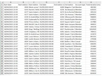
Trip history Bixi makes public all its trip history since its opening in 2014. This work uses data from 2015 and 2016 and covers 10 thousand hours of service. This data is composed for each trip of its start and end station, its start and end time, and the trip duration. The total duration of the trip in milliseconds is also available. These trips are gathered in a csv file and grouped per month (one file per month). The data used in this work was composed of 7 million rows. Montreal network is closed during the winter then there are no trip data during this period. The data used goes from the 15th of April 2015 to the 15th of November 2015 and from the 15th of April 2016 to the 15th of November 2016.
Real-time station status We used for this station data composed by the station position, its capacity, its name and its id. This information is supposed static, even if the operator can modify it during the year (capacity, location and availability). Relocations and shutdowns are always temporary (city work). Bixi tries to place stations always in the same area (a maximum displacement of one city block). Station capacity can change along the year, but only the current capacity is needed in this work. Bixi makes current station information publicly available, they moved it to the GBFS format, as Citybike (New York) and capital Bikeshare (Washington). The GBFS norm definition is available at https://github.com/NABSA/gbfs. Bixi’s data is accessible on the following link https://api-core.Bixi.com/gbfs/gbfs.json
Figure 3.1 Example of a trip file
This format is composed of two data sets : The immutable information and the mutable information. The first one gathers information about the station properties (location, capa-city, ...) the second one gathers the station status. The first data set, accessible at https: //api-core.Bixi.com/gbfs/en/station_information.json presents :
— the id of the station
— the complete name of the station — its short name
— the latitude — the longitude
— the rental payment methods — the capacity Example : { "station_id":"1", "name":"Gosford / St-Antoine", "short_name":"6001", "lat":45.50981958364862, "lon":-73.55496143951314,
"rental_methods":["KEY","CREDITCARD"], "capacity":19,
"eightd_has_key_dispenser":false }
The second data set is accessible at https://api-core.Bixi.com/gbfs/en/station_status. json and presents the station status, i.e. :
— station ID
— number of available bikes
— number of unavailable bikes (blocked, or damaged) — number of available docks
— number of unavailable docks (off or damaged) — a Boolean that is true if the station is installed — a Boolean that indicates if rentals are allowed — a Boolean that indicates if returns are allowed — last connection timestamp
{ "station_id":"1", "num_bikes_available":0, "num_bikes_disabled":0, "num_docks_available":2, "num_docks_disabled":17, "is_installed":0, "is_renting":0, "is_returning":1, "last_reported":1480007079, "eightd_has_available_keys":false }
3.1.1 Bixi private data
Bixi has also access to other data, not available online. Bixi collects information about its infrastructure : stations, docks, bikes, and keys and about its actors : technicians, clients, customer service agents and mechanics. Bixi works with several external companies that manage their data and help them understanding the network status.
3.2 Weather data
Figure 3.2 Example of precipitation file
The weather information is taken from données Canada (don, 2018) and provides data with an hourly precision. The data is composed of quantified measures as visibility, humidity, atmospheric pressure, temperatures and qualitative measures for the weather (rain, snow, fog, . . . ). The meteorological data come from Montreal INTL A station (id 7025251). The data used for this work comprehends the period between 01/01/2015 and 31/12/2016. The data is presented in a csv file with :
— the date and hour
— a quality indicator of the data — the temperature (◦C)
— the dew point
— the relative humidity (%) — the wind direction (per 10 deg) — the wind speed (km/h)
— the visibility (km) — the pressure (kPa) — the wind chill
— the weather (text)
Figure 3.2 shows an example of weather data. We can see that the weather column has a lot of missing data. Next paragraph covers this problem.
Remark : The weather data used in this work is the observed data. However, the model we are going to build is the next chapter is intended to predict future demand and thus should use weather prediction. However, we chose to learn our model on the observed weather. Firstly, because the demand reacts to the real weather and not to the predicted one, secondly because weather predictions three to six hours in advance are quite precise and lastly because learning the model on the predicted weather introduce even more stochasticity in the problem.
3.3 Holidays and National Days
We collected Montreal’s holidays and national days manually on the internet. They were added as two new features, indicating whereas an hour is during a holiday or national day. We differentiate public holidays called national days in this paper and school holidays called holidays.
3.4 Preprocessing
Once the data is collected, it has to be preprocessed. This step aims to shape the data removing gaps and inconsistent values.
3.4.1 Features preprocessing
First we build a feature matrix from the weather and time data. We augment it with holidays and national days. The following operations are computed :
1. Missing values in the weather data are filled with the nearest available value (a maxi-mum distance of five hours is authorized). Missing data was found for weather, wind speed, temperature, visibility, pressure, humidity and wind chill. More than half of wind chill data is absent, this feature is then not considered in the rest of this work. This missing data completion operation is detailed in Section 3.5.
2. Textual weather is transformed into categories : rain, showers, snow, ice, drizzle, fog, cloudy, storm, heavy, moderate and clear.
3. The date time column is split into five columns : year, month, day, hour and day of the week. Due to the evident non-linearity dependence between the traffic and the hour of
the day, categorical variables are introduced for each hour (24 new variables).
4. The plot of trip counts per hour of the week (Figure 3.3) shows three different behaviors, one for the weekend, one for Monday and Friday and one for the remaining days of the week. The literature on bikesharing use categorical variables for week days. They create two (Yoon et al., 2012; Yin et al., 2012; Lathia et al., 2012), three (Rudloff and Lackner, 2014) or seven (Vogel et al., 2016; Borgnat et al., 2011; Li et al., 2015) categorical variables. In this work we choose to use three categorical variables. Then three weeks days categorical variables are created. The first regroups Sunday and Saturday, the second Monday and Friday and the last, Tuesday, Wednesday and Thursday. Days in each category are very similar, then using seven categories instead of three is not interesting as it adds a lot of parameters for a small potential precision improvement. 5. A holiday and a National day columns are added to the data.
This data in represented using a matrix representing for each hour (row) its features (co-lumns). This matrix is used to learn the model.
3.4.2 Objective preprocessing
The trip data is also transformed to get the objective matrix. In this work we model arrivals and departures in a station independently. We suppose that the behavior of arrivals and departures are not related. Therefore we consider them separately. We push this hypothesis even further considering that arrivals and departures are equivalent. This hypothesis supposes that arrivals and departures can be modeled using the same approach. Hence stations are separated into two sub stations, one that counts only arrivals and one that counts only departures. Until Chapter 5, we split stations in two new stations, one that count departures
and one that count arrivals. Complete stations are recomposed in the last chapter to build decision intervals, and model the behavior of a station fills level.
To preprocess trip data, we first aggregated it by stations and hour, in a simple matrix. Then if there are n stations in the network, there are 2 × n columns in the matrix. The objective matrix represents for each hour, the number of arrivals and the number of departures of each station. This column is important because the trip data is not complete : the network is closed during winter. Hence, these hours are excluded from the learning data.
To build this matrix, we choose a one-hour time step. This choice is justified by Rudloff and Lackner (2014) whom proved that it is a good compromise between stochasticity and precision. This time step is also practical, because features are given per hour. This precision is also sufficient for the operator that needs long time prediction up to 7×24=168 hours. We also tried to transform data to improve the performance of algorithms. Section 4.5.1 presents some data transformation as normalization, log transformation (Wang, 2016) and features decorrelation.
3.5 Missing Data
The analysis of weather data showed that there were some missing data. Table 3.1 shows the number of missing values per data column. We found 13 missing hours for all data, probable to station shut down. However, none of these 13 hours were consecutive, hence we filled them using a forward fill method (fill with the data of the previous hour). This approximation is reasonable because of the small variations of meteorological measures between two conse-cutive hours. This estimation neglects possible, but unlikely, exceptional events during the hour. The more problematic point is the number of missing weather values : more than half of the values are missing, then a more accurate analysis is needed.
Table 3.1 Missing data numbers column data missing % data missing
temperature 6 0.05 Humidity 6 0.05 visibility 6 0.05 wind 6 0.05 pressure 6 0.05 wind chill 10133 99 weather 6115 59
To analyze weather missing values we computed the gap sizes (number of consecutive missing values) on the whole weather dataset (train + test). The results are reported in table 3.2. It appears that most gaps are of size 2. The study of the data also shows that most weather values do not vary between three consecutive hours (identical for two gaps over three) i.e. between the hour before and after the gaps. Hence completing the missing values using the nearest available data is justified. This data seems to be recorded every two hours and not every hour.
Table 3.2 gap occurrences
gap sizes 1 2 3 4 5
occurrences 225 2941 1 0 1
3.6 Feature Analysis
In the previous subsections we built the features of table 3.3. In this subsection, we select the significant features.
Table 3.3 Available features for the model
Time features Weather features
Year (integer) Temperature (continuous)
Month (integer ∈ [1, .., 12]) Visibility (continuous) Day of month (integer ∈ [1, .., 31]) Humidity (continuous) Day of week (integer ∈ [1, .., 7]) Pressure (continuous) Hour (integer ∈ [0, .., 23]) Wind (continuous) Monday/Friday (binary) Rain (binary) Tuesday/Wednesday/Thursday (binary) Cloudy (binary) Saturday/Sunday (binary) Brr (binary) National day (binary) Showers (binary)
Holiday (binary) Fog (binary)
Hour 0 (binary) Drizzle (binary)
... Storm (binary)
Hour 23 (binary) precip (binary)
Heavy (binary) Moderate (binary) Snow (binary) Ice (binary) Clear (binary)
features. To build this plot, data is split into categories (for continuous features) and for each category we display its means and its two quartiles. There is one plot per considered feature. The first graphs show a clear dependency between features and trip number. In the last graphs, this dependency is less clear. However the absence of dependency in these graphs does not prove that these features should not be considered. The week-day feature for example is not significant, however its usage is essential to achieve good performances as user behavior changes (distribution of traffic during the day) between week days and week ends. However, these graphs are not a dependency proof. Section 3.6.1 analyze more rigorously the dependencies.
To build a good model is it also important to check the correlation between features as they may cause overfitting, or can influence the interpretation of results. Figure 3.5 represents the correlation matrix between the features. High correlation is shown in red (≈ 1), null correlations in white (≈ 0) and negative correlation in blue (≈ −1). The notable correlations between variables are :
Positively correlated features : — pressure and year
— precipitation and rain — showers and rain
— showers and precipitation
— week day and the categorical variable Saturday/Sunday — temperature and holidays
— drizzle and fog — fog and brr — fog and drizzle
Negatively correlated features :
— the categorical variable Tuesday/Wednesday/Thursday and week day — visibility and humidity
— precip and cloudy — visibility and rain — visibility and precip — temperature and humidity
We can also point out the dependence between hour of the day and temperature and between humidity and visibility. Most of these correlations can be simply explained by dummy va-riables or simple observations. For example, temperature and holidays are correlated because holidays mostly happen during hot months, also cloudy and rain are negatively correlated because when it rains, the cloudy is implied and then not written. These kinds of explanations are valid for most correlated variables. However, they cannot explain the correlation between year and pressure.
This analysis shows some features that add more confusion than they explain the objective. It appears that holidays and cloudy are not highly correlated to the trip number, while being highly correlated to other features. These features are then discarded. Some variables are redundant by construction (dummy variables). Then one possibility between the dummy variables and the continuous one is chosen depending on the model. Even if some strong correlations are still present, we chose to keep most variables to improve the performance, as we try to accurately predict the traffic. Regularizations methods (penalization of big weights) will be used to limit overfitting with correlated variables.
4 5 6 7 8 9 10 11 Month 0 1000 2000 3000 trip number 0 1 2 3 4 5 6 7 8 91011121314151617181920212223 Hour 0 1000 2000 3000 trip number -4 -2 0 1 2 4 6 8 101214161820222426272931 Temperature 0 1000 2000 3000 trip number 98989899999999100100100100101101101101102102102102103 Pressure 0 1000 2000 3000 trip number 1620242832364045495357616569747882869094 Humidity 0 1000 2000 3000 trip number 0 1 precip 0 1000 2000 3000 trip number 0 1 Rain 0 1000 2000 3000 trip number 0 1 snow 0 1000 2000 3000 trip number 0 1 Showers 0 1000 2000 3000 trip number 0 1 Heavy 0 1000 2000 3000 trip number 0 1 Storm 0 1000 2000 3000 trip number 0 1 National Day 0 1000 2000 3000 trip number 0 3 6 9 13161922252932353841454851545761 Visibility 0 1000 2000 3000 trip number 0 1 brr 0 1000 2000 3000 trip number 0 1 Drizzle 0 1000 2000 3000 trip number 0 1 Fog 0 1000 2000 3000 trip number 0 2 5 7 10131518212326293134373942454750 Wind 0 1000 2000 3000 trip number 1 2 4 5 7 8 1011131416171920222325262829 Day 0 1000 2000 3000 trip number 2015 2016 Year 0 1000 2000 3000 trip number 0 1 2 3 4 5 6 Week day 0 1000 2000 3000 trip number 0 1 Holidays 0 1000 2000 3000 trip number 0 1 Cloudy 0 1000 2000 3000 trip number
hour Week day National Day Holidays Year Month Day Hour Temperature Humidity Wind Visibility Pressure Showers snow Rain Heavy Drizzle Fog Cloudy Storm precip brr h0 h1 h2 h3 h4 h5 h6 h7 h8 h9 h10 h11 h12 h13 h14 h15 h16 h17 h18 h19 h20 h21 h22 h23 MonFri TueWedThur SatSun End date Start date hour
Week day
National DayHolidays
Year Month Day Hour Temperature HumidityWind Visibility Pressure Showerssnow Rain Heavy Drizzle Fog Cloudy Storm precip brrh0 h1 h2 h3 h4 h5 h6 h7 h8 h9 h10 h11 h12 h13 h14 h15 h16 h17 h18 h19 h20 h21 h22 h23 MonFri TueWedThur SatSun End date Start date
3.6.1 Feature significance
Figure 3.6 ANOVA results, computed using scipy OLS
To test the feature significance, we used the ANOVA (ANalysis Of VAriance) test. Results are shown in Figure 3.6. This figure shows that, with a 95% confidence (p-value at 0.05, column P > |t|) the number of trips depends on the week day, the national days, the holidays, the month, the hour, the temperature, the humidity, the visibility, the showers, the snow, the drizzle and the fog. The other dependencies were not proven by ANOVA. Therefore the year, the day, wind, pressure, rain and heavy (rain) dependencies, were not significant. However, this analysis tracks only linear dependency and is not able to check more complex ones. Furthermore this analysis has been done on the total number of trips and these features may
be significant for some stations. The correlation between features also makes some features not significant as their influence has already been modeled by the other feature.
This analysis also gives a R2 score of 0.540 to model the total number of trips. This score means that 54% of the variance of trips counts have been explained by the linear regression. This score, gives a first base line for our model. This R2 score is quite low but usual for hu-man behavior studies. This score is computed on the learning data and may be overestimated.
3.6.2 Data analysis conclusions
In this section we completed missing data, selected the features for training and preprocessed the trip data. Table 3.4 presents the features built and validated in this section, with their type. Some of these features are redundant (Hour and Hour i). They represent two options for the learning, only one is selected for each model.
Table 3.4 Selected features for the model
Time features Weather features
Year (int) Temperature (float)
Month (int ∈ [1, .., 12]) Visibility (float) Day of month (int ∈ [1, .., 31]) Humidity (float) Day of week (int ∈ [1, .., 7]) Pressure (float) Hour (int ∈ [0, .., 23]) Wind (float) Monday/Friday (boolean) Rain (boolean) Tuesday/Wednesday/Thursday (boolean) Cloudy (boolean) Saturday/Sunday (boolean) Heavy (boolean) National day (boolean) Showers (boolean)
Holiday (boolean) Fog (boolean)
Hour 0 (boolean) Drizzle (boolean)
... Storm (boolean)