UNIVERSITÉ DE MONTRÉAL
DEVELOPING A RUN-TIME COUPLING BETWEEN ESP-R AND TRNSYS
ROMAIN JOST
DÉPARTEMENT DE GÉNIE MÉCANIQUE ÉCOLE POLYTECHNIQUE DE MONTRÉAL
MÉMOIRE PRÉSENTÉ EN VUE DE L’OBTENTION DU DIPLÔME DE MAÎTRISE ÈS SCIENCES APPLIQUÉES
(GÉNIE MÉCANIQUE) DÉCEMBRE 2012
UNIVERSITÉ DE MONTRÉAL
ÉCOLE POLYTECHNIQUE DE MONTRÉAL
Ce mémoire intitulé:
DEVELOPING A RUN-TIME COUPLING BETWEEN TRNSYS AND ESP-R
présenté par : JOST Romain
en vue de l’obtention du diplôme de : Maîtrise ès sciences appliquées a été dûment accepté par le jury d’examen constitué de :
M. BERNIER Michel, Ph.D., président
M. KUMMERT Michaël, Ph.D., membre et directeur de recherche M. BEAUSOLEIL-MORRISON Ian, Ph.D., membre
ACKNOWLEDGEMENTS
Je tiens à remercier tout particulièrement Michaël Kummert, mon directeur de recherche, pour la disponibilité, le soutien ainsi que la confiance qu'il m'a accordés tout au long de ces deux années de maîtrise.
I am grateful to all the co-simulator project Team members. A special thanks goes to Francesca Macdonald for her dynamism and in memory of these long days spent on debugging the coupling together. I would like to thank Tim Mcdowell for his warm welcome in Madison and his support in helping me getting to know the dark parts of TRNSYS. I wish to thank Ian Beausoleil-Morrison and Alex Ferguson for their contributions and management of the project. Nothing of this would have been possible without them.
Je voudrais remercier également tous les MecBats avec qui j'ai passé deux ans inoubliables à Polytechnique: Aurélie Verstraete, Katherine D'Avignon, Marilyne Rancourt-Ouimet, Marion Perez, Antoine Courchesne-Tardif, Benoit Delcroix, François Adam, Humberto Quintana, Massimo Cimmino, Mathieu Lévesque, Matthieu Grand, ainsi que Michel Bernier.
I wish to thank Westphal Jean-Paul pour m'avoir enseigné le bon usage des "therefore" dans l'écriture de ce mémoire et ses autres nombreuses corrections.
Merci à mes parents pour leurs encouragements ainsi qu'à tous ceux que j'ai côtoyés et qui m'ont soutenu durant toute la durée de ce travail.
RESUME
Dans le cadre de la réduction de l'énergie consommée par les bâtiments, il est essentiel d'être rigoureux dans leur modélisation. Pour ce faire, un grand nombre de logiciels de simulation existe, mais, ces outils sont pour la plupart spécialisés dans un domaine particulier et ne permettent pas toujours de réaliser une analyse complète. Étant donné que tous les domaines (chauffage, climatisation, ventilation, éclairage, acoustique) sont interdépendants, il n'existe pas de plateforme de simulation permettant de couvrir toutes les particularités d'un système avec la même flexibilité, et il est nécessaire de procéder à des combinaisons ou des couplages de logiciels. Ce mémoire décrit la réalisation d'un couplage au niveau de l'exécution entre TRNSYS et ESP-r.
Afin de réduire au maximum les modifications apportées aux codes sources et façonner un outil durable face au développement de chacun des deux logiciels dans le futur, le couplage se fait principalement à l’aide de nouveaux composants recevant et envoyant des données à l'autre programme. L'échange de données est réalisé par une structure à DLLs multiples. En plus de celles de TRNSYS et ESP-r, une troisième DLL chargée d'appeler les deux autres et de contrôler l'échange d'information a été créée. Celle-ci supervise également le contrôle de la convergence et assure l'avancement simultané des deux programmes. Cette DLL qui joue le rôle d’intermédiaire entre les deux logiciels (middleware) est appelée l’Harmonizer.
Une nouvelle catégorie de composants a été mise en place pour le logiciel TRNSYS. Il s'agit des Types Échangeurs de Données (Data Exchanger Types). Ces composants fonctionnent de manière identique aux Types classiques en communiquant à travers leurs entrées et sorties, mais ils sont également capables de forcer le solveur à poursuivre les itérations d'un pas de temps. Cette fonctionnalité est essentielle afin d'obliger TRNSYS à faire de nouveaux calculs lorsque qu'il y a convergence au niveau interne mais que ce n'est pas le cas pour l'autre logiciel. Un composant de cette nouvelle catégorie, appelé Type 130, a été créé spécialement pour le couplage avec ESP-r. Ce dernier assure la liaison et l'échange de données entre l'Harmonizer d'une part et les composants du système dans TRNSYS de l'autre.
Du point de vue de l'utilisateur, il n'y a que peu de changements entre le fait de réaliser un modèle pour une co-simulation et celui pour une simulation n'utilisant qu'un seul logiciel. Les fichiers d'entrée et de sortie sont identiques à ceux d'une simulation standard, et ce pour les deux
logiciels. L'unique fichier additionnel à configurer est le fichier d'entrée de l'Harmonizer contenant les paramètres de la co-simulation.
Ce mémoire décrit le travail réalisée par l’équipe du projet et les contributions spécifiques de l’auteur sont identifiées dans le texte.
ABSTRACT
Rigorous modeling is essential to design buildings and deliver the next advances in energy efficiency and on-site renewable energy production. A great variety of energy simulation programs exists but they are, for the most part, specialized in one particular domain and they do not allow a complete analysis. Because all domains (heating, cooling, ventilation, lighting, acoustic) are interconnected and there is no global simulation environment existing that covers all of the system particularities with the same flexibility, it is often appropriate to proceed with software combination and/or coupling. This Master thesis describes the implementation of a run-time coupling between TRNSYS and ESP-r.
In order to minimize the modifications to the source codes and create a tool able to support future development of each program, new components that receive and pass data to the other program were implemented in the two software programs. A multi DLL structure enables the coupling and exchange of information. A third piece of software, the Harmonizer, launches TRNSYS and ESP-r DLLS and manages the exchange of data. It is also ESP-responsible of the conveESP-rgence handling and controls that both programs march through time together time step after time step.
A new category of components, the Data Exchanger Types was implemented in TRNSYS. These components can work as standard TRNSYS Types and exchange data through their inputs and outputs but they can also impose the solver to continue iterating. This capability is essential to force TRNSYS to do more calculations at a specific time step when it has converged but co-simulation convergence requires more iterations. A component of this new category, Type 130, was created specifically for the coupling with ESP-r. Type 130 exchanges data with the Harmonizer on one side and with the TRNSYS network of Types on the other side.
Testing of basic data exchange validates the data exchange method and the coupling. The co-simulator is able to simulate a complete system with a building modeled in ESP-r and the energy system in TRNSYS.
On the user perspective, there are few changes in implementing a co-simulation model in comparison to a simple simulation model using only one program. Users with some knowledge of both programs will be familiar with the steps required to perform a co-simulation. The input
and output files are the same for the two programs as a standard simulation. Settings of the co-simulation are defined in the Harmonizer input.
This Master Thesis describes the work of the project team, referred to as the Design Team in the text. Specific contributions from the author are identified in the document.
TABLE OF CONTENT
ACKNOWLEDGEMENTS ... III RÉSUMÉ ... IV ABSTRACT ... VI TABLE OF CONTENT ... VIII LIST OF TABLES ...XII LIST OF FIGURES ... XIII LIST OF ABBREVIATIONS ... XVI
INTRODUCTION ... 1
CHAPTER 1 LITERATURE REVIEW ... 3
1.1 Building simulation ... 3
1.1.1 Net Zero Energy Buildings ... 3
1.1.2 Integrated simulations ... 4
1.1.3 TRNSYS and ESP-r ... 6
1.2 Internal coupling ... 9
1.3 External coupling ... 10
1.3.1 The Neutral Model Format ... 11
1.3.2 Sequential coupling ... 12
1.3.3 Run-time coupling ... 13
1.4 Implementation of a run-time coupling ... 15
1.4.1 Master/slave strategy ... 15
1.4.2 Middleware ... 16
CHAPTER 2 ESP-R, TRNSYS AND COUPLING METHODOLOGIES ... 18
2.1.1 Building thermal domain ... 19 2.1.2 Plant domain ... 21 2.1.3 Electrical domain ... 23 2.2 TRNSYS methodologies ... 23 2.2.1 Overview ... 24 2.2.2 TRNSYS Types ... 26 2.2.3 Solver ... 28 2.2.4 Categories of Types ... 30 2.3 Co-simulation approach ... 31
2.3.1 Run time coupling ... 31
2.3.2 Middleware ... 33
2.3.3 Exchange of data ... 34
2.3.4 Harmonizer functions ... 37
CHAPTER 3 SOURCE CODE MODIFICATIONS ... 40
3.1 Modifications in ESP-r source code ... 40
3.1.1 Coupling components ... 41
3.1.2 Coupling subroutine ... 42
3.2 TRNSYS: Creation of a new category of Types ... 42
3.2.1 Objectives ... 43
3.2.2 Data exchanger Types ... 43
3.2.3 TRNSYS kernel main subroutines ... 46
3.2.4 Modifications to the code ... 54
3.3 TYPE 130 ... 60
3.3.2 Type 130 communication process ... 61
3.3.3 Type 130 inputs, outputs and parameters ... 63
3.3.4 Standard and test modes ... 64
3.3.5 Type 130 code ... 65
CHAPTER 4 DEMONSTRATION AND TESTS ... 68
4.1 Preliminary tests ... 68
4.1.1 External data transfer and iteration control ... 68
4.1.2 Data exchange with ESP-r (Test A) ... 69
4.2 Water based heating system (test B) ... 70
4.2.1 System tested ... 70
4.2.2 ESP-r ... 71
4.2.3 Simulation using TRNSYS only ... 71
4.2.4 Results analysis ... 73
4.3 Air based heating system and humidity transfer (test D) ... 75
4.3.1 No humidity source ... 76
4.3.2 Constant humidity source ... 78
4.4 House serviced by a DHW/space heating solar combi-system (test C) ... 80
4.4.1 System tested ... 80
4.4.2 TRNSYS ... 82
4.4.3 ESP-r ... 85
4.4.4 Coupling settings ... 86
4.4.5 Results analysis ... 87
CHAPTER 5 USING THE ESP-R / TRNSYS CO-SIMULATOR ... 95
5.2 Harmonizer input file ... 96
5.3 ESP-r model ... 97
5.4 TRNSYS model ... 101
5.4.1 Creation of TRNSYS input file ... 101
5.4.2 Type 130 Test mode ... 106
5.4.3 Note about controllers ... 107
5.5 Co-simulation ... 108
5.5.1 Running a co-simulation ... 109
5.5.2 Results recovery ... 110
CONCLUSION ... 112
BIBLIOGRAPHY ... 114
ANNEX 1 – ESP-R METHODOLOGIES ... 117
ANNEX 2 – SOURCE CODE MODIFICATIONS IN TRNSYS ... 118
LIST OF TABLES
Table 2-1 Categories of Types ... 31
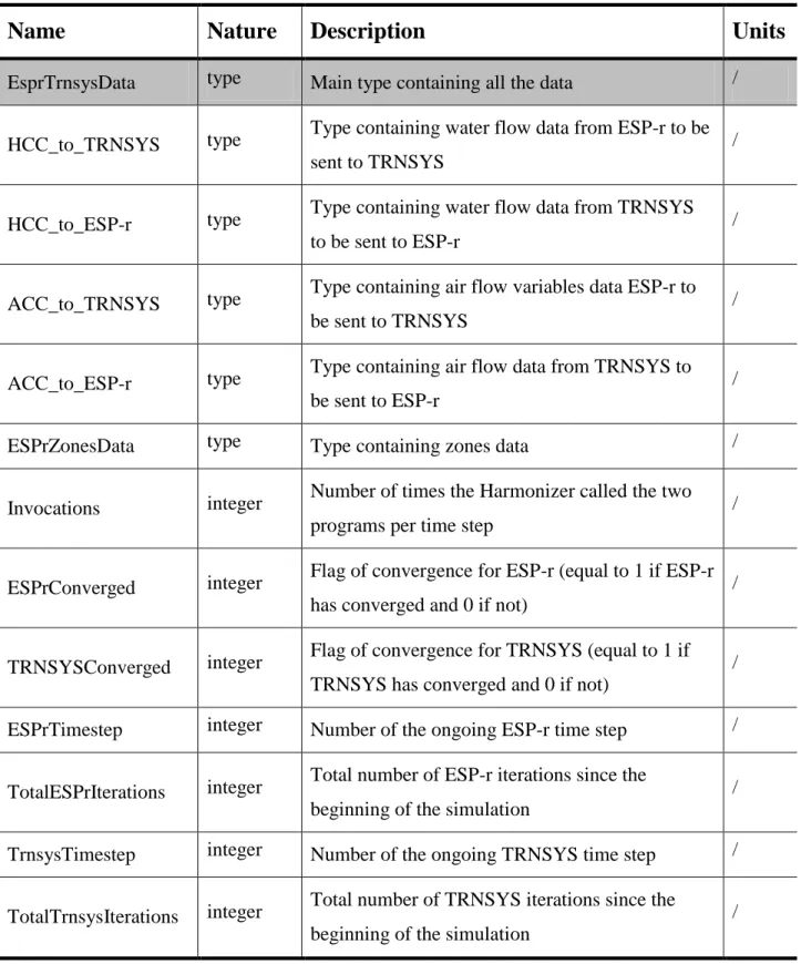
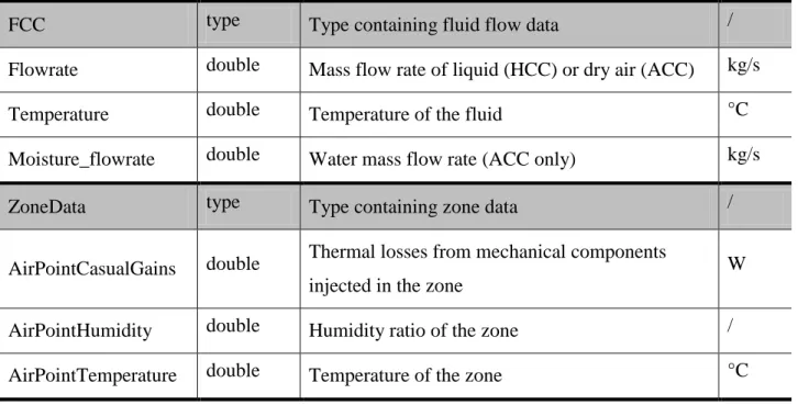
Table 2-2 List of variables and types from the derived data structure ... 36
Table 3-1 Arguments of Exec subroutine ... 49
Table 3-2 “Call” arrays ... 52
Table 3-3 Arguments of Loopex subroutine ... 53
Table 4-1 Radiator model parameters ... 72
Table 4-2 Description of radiator governing equation variables ... 73
Table 4-3 Settings of Test D without humidity source ... 76
Table 4-4 Settings of Test D with Humidity source ... 78
Table 4-5 Parameters of solar collectors ... 82
Table 4-6 Co-simulation parameters for Test C ... 86
Table 4-7 Combi-system co-simulation results (annual simulation) ... 87
Table 4-8 Description of energy transfers ... 89
LIST OF FIGURES
Figure 1-1 TRNSYS Simulation Studio ... 7
Figure 1-2 ESP-r Project Manager interface ... 8
Figure 1-3 Couplings synthesis ... 12
Figure 1-4 Run-time coupling strategies (Trcka, Wetter, & Hensen, 2009) ... 13
Figure 1-5 Loose coupling zig-zag ... 16
Figure 1-6 Interactions between the middleware and the programs ... 17
Figure 2-1 ESP-r's partitioned solution approach (Beausoleil-Morrison, 2011) ... 18
Figure 2-2 ESP-r's building thermal domain finite difference ... 19
Figure 2-3 Heat balance for a zone air CV (Beausoleil-Morrison, 2011) ... 20
Figure 2-4 Heat balance for intra-constructional CV (Beausoleil-Morrison, 2011) ... 21
Figure 2-5 Simulation Studio ... 24
Figure 2-6 TRNBuild ... 25
Figure 2-7 TRNEdit interface and example of a TRNSED application ... 26
Figure 2-8 TRNSYS Type and network topology ... 27
Figure 2-9 Interactions between the main TRNSYS programs and files during a simulation ... 28
Figure 2-10 TRNSYS solution methodology ... 29
Figure 2-11 Sequence of calls to the different categories of Types ... 30
Figure 2-12 Differences in run-time couplings ... 32
Figure 2-13 Data flows between the Harmonizer and the coupled programs ... 33
Figure 2-14 Derived Data Structure ... 35
Figure 2-15 Interactions between the two programs and the Harmonizer (Macdonald, 2012)... 39
Figure 3-1 Coupling components strategy to transfer data to the other program ... 40
Figure 3-3 Calling sequence with Category 6: Data exchanger Types ... 45
Figure 3-4 Original post iterations process ... 48
Figure 3-5 Modifications to the post iterations process ... 58
Figure 3-6 Network of Types including Type 130 ... 62
Figure 3-7 Inputs and outputs organization... 63
Figure 3-8 Coupling components connections ... 64
Figure 3-9 Summary of Type 130 calls and operations ... 67
Figure 4-1 Schematic of test B system ... 70
Figure 4-2 Overview and front view of BESTEST case 600 building ... 71
Figure 4-3 TRNSYS only simulation for Test B... 72
Figure 4-4 Comparison of zone air temperature for two winter days ... 73
Figure 4-5 Evolution of the zone air temperature for the two test cases B1 (right) and B2 (left) . 74 Figure 4-6 Evolution of the zone air temperature and water flow rate with a PID controller ... 75
Figure 4-7 Schematic of test D system without humidity source ... 76
Figure 4-8 - Transient state humidity ratios ... 77
Figure 4-9 - Differences between HR send to the zone and HR of the zone ... 77
Figure 4-10 Schematic of test D system with constant humidity source ... 78
Figure 4-11 Schematic of test C system ... 81
Figure 4-12 TRNSYS simulation for Test C ... 82
Figure 4-13 DHW load profile ... 83
Figure 4-14 Type 130 connections ... 85
Figure 4-15 Zone house model in ESP-r ... 85
Figure 4-16 Connections at the interface between the two programs ... 86
Figure 4-18 Energy transfers in the system ... 88
Figure 4-19 Space heating solar fraction ... 92
Figure 4-20 Domestic hot water solar fraction ... 92
Figure 4-21 System total solar fraction ... 93
Figure 5-1 Co-simulator's input and output files ... 95
Figure 5-2 Harmonizer input file ... 96
Figure 5-3 ESP-r input file ... 98
Figure 5-4 Example of a plant system including coupling components ... 99
Figure 5-5 Coupling components connections: HCC on the left and ACC on the right (Macdonald, 2012) ... 100
Figure 5-6 Example of connections for ACCs (blue) and HCCs (red) ... 100
Figure 5-7 TRNSYS input file ... 101
Figure 5-8 TRNSYS network of Types ... 102
Figure 5-9 Addition of Type 130 to the network of Types ... 103
Figure 5-10 Type 130 parameters settings ... 103
Figure 5-11 TRNSYS network of Types with Type 130 ... 104
Figure 5-12 Simulation parameters ... 105
Figure 5-13 Creation of TRNSYS input file ... 106
LIST OF ABBREVIATIONS
ACC Air Coupling Component
BCVTB Building Control Virtual Test Bed BPS Building Performance Simulation
CV Control Volume
DDS Derived Data Structure DLL Dynamic-Link Library FCC Fluid Coupling Component HCC Hydronic Coupling Component
HR Humidity Ratio
HVAC Heating, Ventilation and Air-Conditioning IAQ Indoor Air Quality
NMF Neutral Model Format NZEB Net Zero Energy Building
OS Operating System
PID Proportional Integral Derivative
PV Photovoltaic
INTRODUCTION
Designing the next generation of energy efficient buildings with on-site renewable energy production to meet the “Net Zero Energy” target requires the use of integrated simulation tools capable of dealing with the level of complexity in the building and the associated mechanical and electrical systems.
A great variety of efficient Building Performance Simulation (BPS) tools exist on the market but they are, for the most part, specialized in one particular domain and lack flexibility or capabilities in other domains. This may affect the accuracy of simulations results as it is sometimes difficult to perform a whole system analysis with one tool. ESP-r and TRNSYS are both powerful simulation programs but their different implementation approaches gave them different strengths. ESP-r is particularly efficient in modeling building physics whereas TRNSYS is more flexible in treating elaborated mechanical and electrical systems. Because all domains (heating, cooling, ventilation, lighting, acoustic) are interconnected and there is no global simulation environment existing that covers all particularities of a system with the same flexibility, combining or coupling simulation programs is often required.
This document presents the work on the development of a run-time coupling between TRNSYS and ESP-r. With funding and guidance from Natural Resources Canada, a Design Team composed of 6 people from Carleton University, Ottawa, École Polytechnique de Montréal, and Thermal Energy System Specialists (TESS), Madison (USA), completed this project. Tasks were divided between the members: the Carleton University part of the team worked on the implementation of the coupling on the ESP-r side and on the implementation of the middleware (known as the Harmonizer), team members from Polytechnique Montréal and TESS carried out modifications to the TRNSYS source code. The whole Design Team was involved during all phases of the project and provided inputs to development work and to the overall coupling strategy, under the supervision of the project leader at Carleton University. This Master thesis describes the methodology and results of the project, with more emphasis on the TRNSYS side. The specific contributions of the author, who was the lead developer for TRNSYS source code changes, are identified in the text.
Thesis organization
First, this document presents Building Performance Simulation combinations and couplings described in the literature. The main approaches are compared. Chapter 1 gives an overview of the couplings methods from basic links and collecting external data to integration of source code and more complex run-time coupling. Chapter 2 presents the calculation methodologies of TRNSYS and ESP-r and a description of the co-simulation approach selected by the Design Team. Chapter 3 details the implementation of the coupling and the modifications to each program source code. The ESP-r part is briefly commented, while TRNSYS source code changes are presented in details with the source code provided in an Annex.
Chapter 4 reports on the various tests that were performed to confirm the proper operation and the usefulness of the proposed co-simulator. Results demonstrating the coupling capabilities from the very basic data exchange tests to complete co-simulations are presented there. Chapter 5 describes how to perform co-simulations from a user perspective, and leads to the final conclusions of this work.
CHAPTER 1
LITERATURE REVIEW
This introductory chapter presents an overview of the current work in building performance simulation and couplings between software programs. First, the need for integrating building simulation programs and different approaches are presented. Then, different coupling methods are discussed.
1.1 Building simulation
The design of buildings and mechanical systems aims at saving energy while maintaining or improving occupant comfort. Integrated Building Performance Simulation (BPS) tools play an important role in assessing the energy and economic performance of design options. They must be efficient and adapted to more and more demanding building standards, codes and certification programs. The end of the section presents two of the major programs in that domain, TRNSYS and ESP-r.
1.1.1 Net Zero Energy Buildings
Design of buildings in the near future will be oriented towards the Net Zero Energy Building (NZEB) target. Stricter energy efficiency regulations are already taking shape for the next decades. In the USA, the goal of net zero for every new commercial building is set to 2030 by the Energy Independence and Security Act of 2007 (EISA 2007). The European Union is even more demanding in the reduction of energy consumption with the Energy Performance of Building Directive (EPBD) that imposes a neutral energy balance for every new construction by 2020. These texts are ambitious, however they lack precision on the definition of Net Zero Energy buildings, as well as on the methodology to design those types of buildings (Marszal et al., 2011). Currently, several definitions of NZEB exists (Torcellini, Pless, & Deru, 2006) but in order to apply these new laws, a rigorous design methodology will be needed. This will also require the creation of new buildings and systems simulation tools and/or modifications of the current ones to respond efficiently to these energy saving constraints.
Several methods of defining the total energy balance of buildings already exist. The majority uses the primary energy consumption in their calculations. They differ for example on the period of simulation: they mostly consider a period of one year but this period can vary from a month to the entire life cycle. A few of these approaches only consider thermal and electrical energy used to operate the building, while others extend the energy balance to account for the energy required during the construction process (including embodied energy for all construction materials). A commonly used indicator of the net zero energy target is the ratio between the building energy consumption and the on-site renewable energy production. There is no consensus on a “best” methodology at this stage, each of them focuses on slightly different aspects of the problem. The design of NZEBs and the evaluation of their performance must be adapted to the selected methodology.
BPS tools must be adapted to these requirements and allow to improve energy efficiency at the building level, as well as to integrate advanced Heating, Ventilation and Air-Conditioning (HVAC) systems and on-site renewable energy systems.
1.1.2 Integrated simulations
Rigorous modeling is essential to design buildings that will meet the very ambitious energy efficiency targets described above. It is essential to treat buildings and systems, at the same time to get the best optimization (Hensen, Djunaedy, Radošević, & Yahiaoui, 2004). Using a systemic modeling approach during the design phase, allows harmonizing all of the key domains of building construction from the engineering part to the architectural part. This leads to a design optimizing both the energy consumption and the comfort of occupants.
Bazilian et al. (2001) illustrated the need of integrated simulations in modeling co-generation photovoltaic collectors and the strong link between architecture and system design. A façade configuration with pre-heating of the supplied air is presented by the author who explained that such a system would also impact substantially the architectural domain. It is therefore necessary to tackle every domain at the same time. Although several existing systems have proved the efficiency of that type of collectors, more detailed tests must be performed. The lack of modeling tools capable of performing holistic simulations is a barrier to research projects in that field. A
great variety of building simulation programs exist but they are, for the most part, specialized in one particular domain and they do not allow a complete analysis. All domains (heating, cooling, ventilation, lighting, and acoustics) are interconnected. Considering that there is no global simulation environment that covers all of the system particularities with the same flexibility, researchers and practitioners must resort to software combination and/or coupling (Citherlet, Clarke, & Hand, 2001). There are four possible strategies:
- Stand-alone programs
In this case, a new simulation has to be created for every particular domain of the analyzed system, each time using different software. Thus, this leads to redundancy issues and it can be very fastidious as every time design parameters change in a domain, all the simulations have to be modified and re-run another time. Another constraint for that kind of technique is that the user has to be familiar with all the different programs used.
- Interoperable programs
The programs share the same source of information. This can be done following two approaches: a. Exchange of an entire model or a part of the model
b. Sharing of the model: each program uses information it needs from the common and unique model.
The second approach removes the redundancy but, in any case, the user needs to be familiar with all the programs as well. Although there can be a loss of time dealing with all the different simulating tools, we are closer to the reality of a global project. This strategy clearly represents the interactions between all the actors: engineer, architect, etc.
- Integrated programs
In this scenario, several domains are modeled and simulated with the same program. The evolution of the program is simplified as it does not depend on other applications. Moreover it does not need any data exchange format and necessitates only one model grouping all the project information.
- Coupled programs
The users have to be familiar with both tools in this case too. Calculations are done simultaneously by two or more programs that also exchange data. Several possibilities of
couplings exist and they will be presented below. This solution offers the best flexibility to the users as it gives them the possibility to benefit from the new functionalities added to the coupled programs.
1.1.3 TRNSYS and ESP-r
Simulating buildings and energy systems in a global approach can be performed efficiently by coupling existing programs specialized in different domains. This requires to choose appropriate programs, not only powerful in their specific domain but also complementary. Two different programs that seem to satisfy these conditions are presented briefly below.
a. TRNSYS
TRNSYS (TRaNsient System Simulation program) is a complete, modular and flexible program for systems simulations (Klein et al., 2010; Keilholz, 2002). The program allows modeling from simple to very complex mechanical plants with varied control systems. The standard libraries contain around 60 components in different domains: HVAC, controls, storage, solar equipment, etc. This list can be completed by additional libraries but also custom-made components that users can create themselves, requiring some Fortran, C or C++ coding skills. TRNSYS is customizable, can be expanded relatively easily, and it can simulate a large number of very specific systems. In addition, it has a user friendly interface for generating projects (Figure 1-1). Components used in the simulation are selected and added to the workspace by a drag-and-drop process before being connected and setup by the user.
Figure 1-1 TRNSYS Simulation Studio
The simulation environment allows modeling multi-zone buildings. Another possibility of the software is to create, via a specialized editor, redistributable applications. It is particularly intended to develop simplified simulation tools, which can then be freely distributed to users who do not possess a TRNSYS license (Klein et al., 2010).
b. ESP-r
ESP-r is an Open-Source energy modeling program for buildings. Dealing with thermal, acoustic and energy performance, it is a comprehensive integrated energy modeling tool. It helps reducing energy use and emissions, and optimizing the occupant comfort. The source code base can be compiled to run the program on several operating systems: Linux, MacOS, Windows/Cygwin and Windows.
After 30 years of development, ESP-r is a powerful engine (Clarke, 2001) which has proved to be very efficient in the modeling of buildings (Strachan, Kokogiannakis, & Macdonald, 2008). Nonetheless, the program lacks of flexibility when it comes to simulate mechanical systems. This may prevent users from addressing the design of global systems (building + HVAC components). The configuration of controls can be a very complex task. Moreover ESP-r does not have a large list of energy systems components as we can find in other simulation programs such as TRNSYS.
Figure 1-2 ESP-r Project Manager interface
Given the functionalities and specificities of TRNSYS and ESP-r, the flexibility of systems network configuration for the first one and the comprehensive BPS aspects for the second one, a coupling of these complimentary tools would provide results with increased value to those obtained with each individual program.
a. Comparison of ESP-r and TRNSYS
ESP-r and TRNSYS are both tools that allow running dynamic simulations for buildings and energy systems but they have different modeling approaches. Based on a report contrasting the capabilities of several building energy performance simulation programs (Crawley, Hand, Kummert, & Griffith, 2005), a comparison giving a more precise review of the strengths and weaknesses of two programs is presented below.
The most rigorous program in the treatment of the building physics is ESP-r. The program integrates features that are not available in TRNSYS. It uses multi-sided polygons to define constructive elements. It also handles CFD modeling. When it comes to implement very specific types of constructive solutions, ESP-r presents a wide range of materials with models of phase
change materials or transparent insulation. Moreover, ESP-r has the ability to simulate daylighting illumination and controls with its link to Radiance. With all these capabilities, ESP-r possesses more than TRNSYS the comprehensive BPS aspects.
TRNSYS has a larger library of components than ESP-r. This is particularly the case for primary HVAC components (boilers, chillers, etc.). It is also easier for the users to create new components by developing personalized Types and add them to the existing list of components. TRNSYS’s modular nature based on components (“Types”) also makes it easier to implement specialized control strategies. The ability to develop new components relatively easily and the flexibility offered in combining them into systems and in defining control strategies make TRNSYS well suited to model innovative systems
1.2 Internal coupling
The first option to couple two programs is to combine their source codes. In most of the cases the coupling is done by adding a part of one program code to another. This may be for instance a component modeling a piece of mechanical equipment that we want to model in another environment.
In 1999, Dorer and Weber integrated COMIS source code in TRNSYS. COMIS is a ventilation and contaminants transport simulator for multi zone buildings. This coupling enables to take into account the interaction of air flow rate and transport of contaminants in the modular systems and buildings simulation program. Indoor Air Quality (IAQ) is closely interrelated with thermal comfort and energy performance and must be considered in a holistic design approach. A new component (Type 57) was added to TRNSYS with a re-implementation of the COMIS source code. It is intended to work in combination with the thermal multizone building component (Type 56) and exchange data (e.g. temperature, flow rate) every iteration, similarly to all TRNSYS components connected through their inputs and outputs. While some convergence problems were identified in case of an important stratification of the air in a zone, a study on effects of night cooling on a building proved that the coupling allows new possibilities of simulations and offers a better help to architectural conception (Dorer & Weber, 1999).
On the other hand, some of the existing TRNSYS components in the HVAC and electrical domains have been integrated into other simulation tools. In 1991, Hensen re-implemented a TRNSYS component (known as Type 260) modeling an aquastat controlled heater into ESP-r (Hensen, 1991) The parameters/inputs/outputs structure of TRNSYS components had to be adapted to the ESP-r engine methodologies. More recently, in 2009, a general method to convert components from TRNSYS to ESP-r has been developed (Wang & Beausoleil-Morrison, 2009). The tool, known as the “TRNSYS wrapper”, makes it easier to incorporate a TRNSYS Type in ESP-r by compiling the code of the component with the source code of ESP-r. The coupling approach used here is the process model interoperation, since both programs use the same model. A few modifications to the source code are required but they have been minimized as much as possible for this work. For someone who has skills in TRNSYS and ESP-r, creating a new component with the “wrapper” based on the TRNSYS source code should only take a few hours, which is reasonable considering that the solvers of the two programs use very different methodologies. ESP-r solves a global matrix system whereas TRNSYS solve equations sequentially, component by component.
Internal coupling helps to add new capabilities to programs by reusing other programs models, but it requires substantial source code changes. It can only be performed by users knowledgeable in the two programs and in computer programming. Another major drawback of the method is that the source code embedded into the other program is decoupled from the original source code, so that any enhancements or bug fixes will have to be adapted again.
1.3 External coupling
There are different strategies to implement an external data exchange between different simulation programs. The choice can be driven by a variety of factors: the need of a small simulation run time, the accuracy of the results, the amount of modifications to the source code. The most common ways to implement externals couplings based on previous works are presented and discussed below.
1.3.1 The Neutral Model Format
Prior to thinking of how the programs are going to communicate, it is important to define what is going to be exchanged. Indeed, simulation programs often do not use the same format or units for their model data. Software A may calculate energy in Joules while a software B would use Watt-hours. The approach in modeling the same component can be also be completely different. A radiator is for example modeled by a node in a state-space matrix in ESP-r, whereas in TRNSYS it is a black box with a temperature and a flowrate as inputs and calculated flow temperature and power as outputs. In another case we can have two programs simulating two separate aspects of a model as acoustic and thermal effects. The model and its properties are the same for both programs but data needed by each program to do its calculations may differ.
The concept of the Neutral Model Format (NMF) was created in order to simplify the data sharing and compatibility (Nataf, 1995). The file gives all the information that characterizes a system in a generic way. It contains systems of differential and algebraic equations describing the model with a listing of all the variables. The name and description of the model and the variables are also present in the NMF. The objective is to enable the sharing of the model file and exchange of data between several programs. Translators are then in charge of collecting data needed by each program and making the unit conversion if necessary.
The independent format may be more complicated to understand for an experienced programmer, but the advantage of NMF is that it can be read more easily by a large number of programs. More importantly, it allows the programmer to focus on the accuracy of the modeling rather than on writing computer code. Several NMF components such as a solar collector, a multi-layer wall, a thermal zone were created and have proven their efficiency. Vuolle and Bring also proposed a whole library of NMF components regrouping zones, walls, windows and controllers (Vuolle & Bring, 1995). Their work demonstrated that using NMFs reduce the implementation time and improve the efficiency of simulations. Moreover the general model format appears to be a robust and maintainable solution as it is completely separate from the development of the programs.
1.3.2 Sequential coupling
In a paper published in 2005, Djunaedy & Hensen gave an overview of the different possibilities for coupling programs. Unlike internal coupling which is used in order to improve a software program by adding new capabilities, external coupling is relevant when the objective is to share a simulation between two existing programs. It can be the case in modeling different domains in different programs. As shown in Figure 1-3, external couplings can be divided in two categories: sequential couplings and run-time couplings. In the first category, one program is executed after the other. The results obtained with the first program launched are then used in the simulation run with the second program. To improve the precision of the results it can be necessary to repeat the process a few times and use the results obtained with one program in the simulation run with the other one.
Figure 1-3 Couplings synthesis
The advantage of an external coupling is that the source code of each program is already written, tested and validated. Coupling the programs externally can save substantial time and money in comparison to internal coupling which requires source code changes. This coupling method is easier to maintain as both programs will benefit from bug fixes and enhancements by their own developers. External coupling Internal coupling Sequential Run-time Loose Strong
1.3.3 Run-time coupling
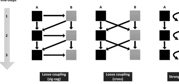
The most complete way to implement an external coupling is to run the programs at the same time and have them communicate during the simulation. This approach is known as run-time coupling. Three possible strategies to implement run-run-time coupling are shown in Figure 1-4.
Strong coupling Loose coupling (zig-zag) Loose coupling (cross)
Figure 1-4 Run-time coupling strategies (Trcka, Wetter, & Hensen, 2009)
"The circles represent the subsystem’s state at a specific moment in simulation time. The dashed arrows indicate which coupling data (time-step wise) are available to each subsystem before the time-step calculation is performed. The full-line arrows indicate the update of state variables." (Trcka et al., 2009)
- Loose coupling (zig-zag)
In loose couplings programs do their own calculations and exchange data only once per time-step. Regarding "zig-zag" coupling (Trcka et al., 2009), one program is executed after the other. E.g.: Program A begins and proceeds with its calculations for the first time-step. Once it has converged, it sends its results to Program B that performs its iterations for the same time-step. In the meantime Program A waits until Program B converges. When Program B is done with its own calculations, it sends data back to Program A which proceeds to the second time-step. The same procedure is executed for each time-step (Δt).
A coupling at the time-step level based on this approach has been made between ESP-r and the lighting simulation program Radiance (Janak, 1999). At each time-step ESP-r calls Radiance and provides it input data. ESP-r waits then until the end of Radiance's iterations, collects the results and uses them in its simulation. Data transfer happens through a temporary text file where the calculated internal illuminance is written by Radiance and read by ESP-r.
- Loose coupling (cross)
For that type of coupling the programs exchange data at the end of each time-step. These pieces of information are then used as input data for the following time-step. Each program performs its own calculations on its side and once the two programs have converged, they both send their results to each other. “Cross” and "zig-zag" couplings deliver improved accuracy compared to sequential coupling, because they exchange data at every time-step. In sequential coupling the whole simulation is executed twice, once with one program and another time with the other. In this particular example, the frequency of data exchange is one time per time-step, but it can be extended to decrease the simulation running time. This will depend on the precision of the results wanted (Trcka, 2008).
- Strong coupling
In a strong coupling implementation, there are iterations between the two programs at each time-step (Trcka, Hensen, & Wijsman, 2006). The programs exchange data several times per time-time-step until an overall convergence is reached. Once the whole system has converged the two programs proceed separately to the next time-step and the same "double" procedure of iterations is done until the end of the simulation. This method should deliver a better accuracy at the cost of increased running time, as a higher frequency of the data exchange will result in more iterative simulation calls. This strategy is mentioned in the literature but, according to our literature survey, it has never been actually implemented between two or more complex Building Performance Simulation (BPS) programs.
1.4 Implementation of a run-time coupling
A run-time-coupling is the best solution when existing programs are efficient in a certain domain but not complete enough to be used for a comprehensive energy simulation. This process model cooperation can be implemented in two different ways: the master/slave strategy or the addition of a middleware.
1.4.1 Master/slave strategy
The choice of the co-simulation strategy implies to define which program will have the control of the whole simulation, which program will wait for the other's data, which one is going to impose input data to the other, etc. For the "master and slave" or "base program/external program" approach one program has the control of the other. It is the case for the coupling between ESP-r and Radiance (Janak, 1999) mentioned before where the lighting simulation program is commanded by ESP-r. A coupling of TRNSYS and EnergyPlus realized in 2009 is also based on this subordination relationship between the two programs. Figure 1-5 illustrates the interactions between the two coupled programs and the differences of each program operations sequence for a time-step (Trcka et al., 2009). The "master" program sends data to the "slave" program at the first iteration of the time-step and then waits for the return of data. The "slave" program sends back once it has converged for the time-step. This strategy is particularly adapted to the "zig-zag" coupling coding as one program is executed after the other.
Figure 1-5 Loose coupling zig-zag
1.4.2 Middleware
Another concept of implementation of a run-time coupling that can be found in the literature is the creation of an additional piece of software: the middleware. Also named "mediator" (Gamma, Helm, Johnson, & Vlissides, 1995), its role is to centralize all the communication between the coupled programs. The schematic of Figure 1-6 presents the interactions between all the programs. yes yes TI M E ST EP O P ER A TI O N S
First iteration of the time-step ? Send data to B Calculation of iteration n A (master) A (master) Receive data from B First iteration calculation Convergence ? no no yes yes no no yes yes
First iteration of the time-step ? Receive data from A Calculation of iteration n B (slave) B (slave) First iteration calculation Convergence ? no no yes yes no no Send data to A Proceed to next time-step Proceed to next time-step
Figure 1-6 Interactions between the middleware and the programs
The middleware simplifies the data transfer handling. Instead of communicating with each other, all programs exchange information with only one program that monitors fluxes of data. It is an efficient way to centralize all the constraints and control functions in the middleware. Gamma et al. (1995) described the simplification of the information exchange by "one to many interaction" instead of "many to many interactions".
An example of the implementation of a middleware in an energy simulation programs coupling is the Building Control Virtual Test Bed (Wetter, 2008, 2011). It is an interface of different simulation tools enabling data exchange. It offers the possibility to link EnergyPlus to other tools and it is therefore meant to be used for testing integrated buildings energy systems and controls. The middleware has its own interface where the user can choose the co-simulation and controls settings. It also has the functionality to analyze the results, print out them graphically and write reports. The coupling approach is based on the "zig-zag" loose coupling concept and there are no iterations between the programs.
Middleware
CHAPTER 2
ESP-R, TRNSYS AND COUPLING METHODOLOGIES
This chapter includes a review of ESP-r and TRNSYS methodologies and calculation approaches. The main similarities and differences that helped define the guidelines of the coupling implementation will be emphasized. This is followed by a description of the coupling design of the two simulation programs.2.1 ESP-r methodologies
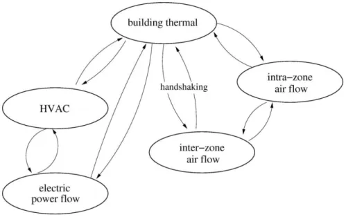
Figure 2-1 ESP-r's partitioned solution approach (Beausoleil-Morrison, 2011)
ESP-r solves the different equations of a simulation using a partitioned solution approach. The problem is solved by discretization in several domains calculated separately. Each domain possesses its own solver that has its own way to solve the equations of the model. The partition into domains as shown in Figure 2-1 includes the building thermal domain, electric power flow, inter zone air flow and intra zone air flow. In order to deal with the relations between the domains and to consider the interdependencies, data is exchanged between the solvers once at every time step. There is an exception for the plant and the electrical domain where iterations can occur within the time step.
2.1.1 Building thermal domain
The building thermal domain is treated with numerical discretization of the model governing equations. The solution is then simultaneously computed by calculating the heat-balances of the whole system. This is essentially done by finding the energy flows with finite difference and control-volume (CV) heat-balances.
Discretization of the model
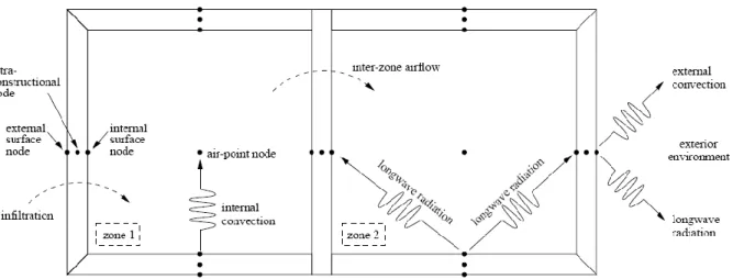
The first step is the discretization of the entire model into finite differences nodes. As presented in Figure 2-2, nodes represent air volumes of the building, fabric components, interfaces or plants components.
Fabric components include walls, windows, roofs, floors. Depending on their composition and the number of material layers, they may be modeled by several successive nodes.
Interfaces model the behavior of the junction of fabric components and air volumes. They represent properties between a solid and a fluid such as the internal or external faces of walls.
Figure 2-2 ESP-r's building thermal domain finite difference discretization and inter-nodal heat flows (Beausoleil-Morrison, 2011)
Heat balance solving
The second step is the elaboration of the heat balance for each node. Figure 2-3 and Figure 2-4 show respectively the heat balances with the energy flows implemented for a zone air CV and a node from a fabric component. The amount of thermal energy entering, leaving and created in the node is equated. The equations are then modified and approximated in their algebraic and discrete form.
infiltration
Inter-zone air flow
0 J S = 1 S = 2 S = 3 S = 4 q 0 -> I q J -> I I { } { } { } { } { }
{ } { } { }
Figure 2-4 Heat balance for intra-constructional CV (Beausoleil-Morrison, 2011)
Since all nodes are interconnected due to the interdependencies between the components of the building, the pooling of the equations results in an equation set describing the whole system. The solution is finally calculated simultaneously for every node time-step per time-step. At a given time, the resolution of the equations gives the thermal state for each node as well as the heat flows to and from that node.
2.1.2 Plant domain
There are two different possibilities for the user to implement a plant in ESP-r: an ideal plant system or an assembly of selectable components. In both cases the user has to specify how the system is controlled.
Ideal plant
With this configuration, users are able to implement an “ideal” plant system, which will respond exactly to the needs of the building in term of heating and cooling. It does not necessitate detailing all the plant components; only the control of the HVAC system is modeled.
The only indication the user has to enter in the program is how the system is controlled. The variable to control (actuator) and the variable that is sensed by the controller (sensor) have to be specified first. The actuator can be an air point of a zone, a surface, a convective and/or radiative
I
I-1 I+1
heater, and/or a location in a fabric component to model the effect of a radiant slab for example. The sensor may be the temperature of one or more zones, external temperature, outdoor wind conditions (speed, direction), the solar radiation (diffuse, direct) or relative humidity. At that point, the control law needs to be specified: heat injection/extraction with fixed capacities, on/off behavior, constant volume with variable temperature, PID controller or free floating without any mechanical heating or cooling.
The ideal plant allows calculating the loads of buildings relatively easily but it may lack precision for detailed simulations as it does not reflect the effects of real components. The response time of a radiator, for example, or the limit to its power output, cannot be taken into account. With this ideal approach the HVAC system is treated with steady-state models
Explicit HVAC
Instead of using the ideal configuration, the user can create the complete network of plant components of the system. A library including tanks, boilers, pumps, heat exchangers, and other mechanical components allows the user to select the needed components for the system he wants to simulate. Their parameters can be modified and for some of them input data is also needed. Components then have to be assembled and in the same way as for the ideal plant, a control strategy needs to be implemented.
Every component is modeled by one or more control volume(s) (CV). A set of mathematical equations representing the behavior of the component are written for each CV. They are used to calculate the energy and the mass exchange between the other connected components and the zone(s). The equations of energy conservation used for all plant components take the following general form:
∑ with:
the mass of the Control Volume the time
the heat capacity an energy flows
Depending on the component, the calculation of the energy flows and generation can be calculated in different ways. Physical (first principle) or empirical approaches may be used. The equations are then solved by a direct solution approach and there are iterations until convergence is reached.
There is a coupling with data exchange between the HVAC domain and the thermal building domain. It allows taking into account the interactions between the two domains. The data transfer is performed both ways once per time step: the building domain is solved at a given time step, calculated temperatures are sent to the HVAC plant domain, which is then solved for that time step. Calculated heat transfer rates from the HVAC plant are then sent back to the building domain which will use them at the next time step. There are no iterations between the two domains within the time step. This coupling between the two domains within ESP-r is a form of “loose zig-zag” according to the nomenclature described above.
2.1.3 Electrical domain
The electrical domain is treated as a network of electrical components and nodes. The components may be cables, transformers, inverters, etc. The nodes are used to calculate the electrical variables: voltages, currents and power. A Newton-Raphson based solver is used to solve the electrical energy balances for all the nodes.
The electrical domain can be coupled to other domains as the HVAC, e.g. in the case of a mechanical component producing or consuming electricity (pump, electric heater, co-generation device).
2.2 TRNSYS methodologies
TRNSYS solving methodologies are different from those implemented in ESP-r. Whereas ESP-r uses more a global approach and calculates a general solution within each domain and then implements a loose coupling between the domains, TRNSYS separates the problem and solves it one component at a time, then performing overall system iterations until all components (and therefore all domains) converge simultaneously.
2.2.1 Overview
The TRNSYS software suite includes 3 different interfaces: the Simulation Studio, TRNBuild and TRNEdit.
Simulation Studio
Figure 2-5 Simulation Studio
The simulation studio is the main TRNSYS interface. It generates the simulation project files. This is where all the components of the mechanical system are assembled into a complete model. The components, known as TRNSYS “Types”, are linked together and form the system network. The Simulation Studio executable allows modifying the simulation settings as the simulation running time, the length of time steps and convergence criteria. When the system is configured and simulation parameters are set, the TRNSYS input file (a text file known as the “deck” file) can be created and the simulation launched directly from the Simulation Studio. In the TRNSYS jargon, each instance of a Type, i.e. each component in the assembled simulation, is called a “Unit”. So each component icon in Figure 2-5 corresponds to a Unit.
TRNBuild
Figure 2-6 TRNBuild
This interface is used to define multi-zone building models. Here, all the characteristics of buildings as material, zones, ventilation, loads, etc. can be defined. The interface is dedicated to configuring parameters for the multi-zone building model in TRNSYS, known as Type 56. The configuration and the properties of the building are saved in text files written by TRNBuild, which are then read by Type 56 during a simulation. Version 17 introduced a link between TRNBuild and Google Sketchup through a plugin known as TRNSYS 3D. This plugin enables to define the geometry of the building and the different zones by drawing them in Sketchup instead of entering their description in TRNBuild. The Sketchup drawing is translated by the plugin and imported into TRNBuild where non-geometrical characteristics (e.g. schedules) can be defined.
TRNEdit
Figure 2-7 TRNEdit interface and example of a TRNSED application
The TRNEdit interface allows to edit the TRNSYS input file (“deck” file). This can be useful to perform parametric runs that are not supported by the Simulation Studio or to create stand-alone redistributable programs with their own simplified interface. These stand-alone executables are called TRNSED applications. They offer the possibility to users that do not have a TRNSYS license to simulate some predefined energy systems. The main restriction of these applications is that users can only change selected simulation parameters accessible from pull-down menus or text boxes. They do not have access to an interface to reconfigure a simulation such as the Simulation Studio.
2.2.2 TRNSYS Types
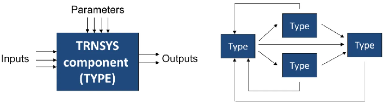
The Types are all the components used in a TRNSYS simulation. They are characterized by 3 categories of variables. The parameters are defined once by the user and remain constant over time. The inputs and outputs represent data that can be exchanged with other components from the simulation. The value of a Type input can be the output of another component when they are connected together. If an input is not connected it will keep its initial value specified by the user. Outputs are the results of the Type calculations. Some other components may need these results as an input variable so a connection can be made between the Types. For each Type, an input can have only one connection with the output of another Type but an output of a Type can be connected with one or more inputs of other Types. An illustration of the creation of a Types network is proposed in Figure 2-8.
Figure 2-8 TRNSYS Type and network topology
There is a large variety in the nature of Types. They do not only represent mechanical components but also a large choice of so-called utility components that do not represent actual equipment but are useful to the simulation (e.g. weather data readers). The main groups of components are listed below:
- Mechanical and electrical components
They are the standard and most used components. They represent real components as a stratified storage tank, a solar collector, a heat exchanger, etc.
- Controllers
These components are used to set the control strategy of the system. Thermostats, differential controllers, PIDs are for example included in the controllers library. - Building and loads
They include different building models, from degree-day analysis to detaile multi-zone building, but also components applying pre-calculated loads to a flowstream. - Outputs
Components of this group define the output files of the simulation. What results should be written to a file (“printed” in TRNSYS jargon), plotted, integrated; the period and the frequency of the results can be specified with these components. - External file readers
They include the components that are specifically used to read data from external files. The most frequently used Type from this group is the weather data reader and processer, but generic data readers can be used to read any text file (e.g. schedules or pre-calculated loads).
- Utility
All other manipulations, operations on data can be handled by this group of Types. They also include Types exchanging data with other programs as EES, Matlab, Comis, etc.
The flexibility of the TRNSYS structure enables users to add their own Types to the standard library of components, largely coded in Fortran. However, any programming languages that are compatible with the Microsoft Windows shared libraries structure (Dynamic-Link Library, or DLL) can be used, e.g. C++
2.2.3 Solver
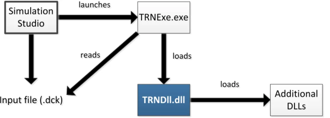
The TRNSYS engine has a structure of shared libraries also called Dynamic-Link Libraries (DLL). When the TRNSYS executable, “TRNExe.exe”, is launched (generally by the Simulation Studio), it reads the simulation input file, the “deck file”, and calls the TRNSYS main DLL, “TRNDll.dll”. The process is presented in Figure 2-9.
Figure 2-9 Interactions between the main TRNSYS programs and files during a simulation
TRNDll.dll contains the source code of TRNSYS. It contains two parts: the kernel (solver routines) and the Types (TRNSYS components). Some components such as user-written Types or Types from commercially available additional libraries do not have their code compiled in the
Input file (.dck)
Input file (.dck) Additional
DLLs Simulation Studio TRNDll.dll TRNExe.exe launches launches loads loads loads loads reads reads
main DLL. They are compiled into additional DLLs that are loaded by the main DLL (TRNDll) as required.
TRNSYS implements two different solvers. Only the default solver, known as “solver 0” (successive substitution) is discussed in this document. During a simulation, Types subroutines are called one at a time by the kernel. Information from some Types’ outputs is passed to the inputs of connected Types. For the kernel, each component is treated as a black-box and it does not make any assumption on what the Types calculate and what is the nature of their inputs and outputs. Figure 2-10 shows the relations between the kernel and the Types. As the components exchange data, more than one iteration may be needed at each time step. Every Type is called at least once at the beginning of a time step and additional calls are performed by the solver as required. Convergence is checked on the variation of the input values of each Type. Types whose inputs have changed more than a given tolerance compared to a previous iteration are called again. This is repeated until the change between the values of two successive iterations is lower than the specified tolerance. Types that do not have been called at some iteration because their inputs did not changed are not blocked and can be called again if their inputs change in future iterations. When all Types have converged TRNSYS proceeds to the next time step.
Figure 2-10 TRNSYS solution methodology
A maximal number of iteration per component at each time step is defined by the user to prevent infinite loops when the solver does not converge. If this number is reached, the kernel proceeds to the next time step but writes a “warning” message indicating that a component did not converge at a certain time. Excessive non-convergence warnings will trigger an error message and stop the simulation.
2.2.4 Categories of Types
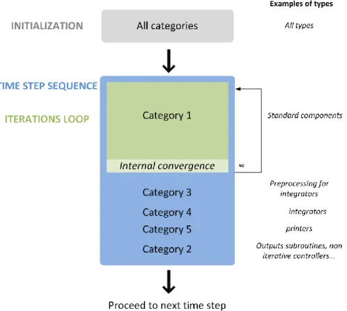
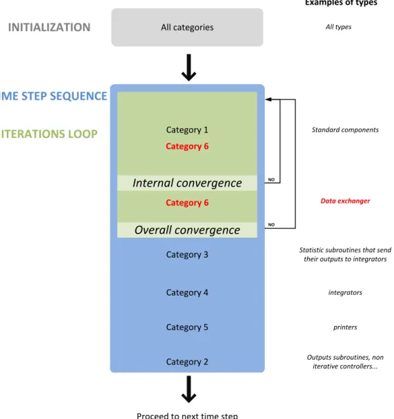
Previously, we saw that the nature of the Types can be very different. Some of them are standard mechanical components that must be called as soon as time has been incremented or their inputs have changed. Other components such as data readers or printers should only be called at the beginning or at the end of a given time step. Different categories of Types are defined in TRNSYS to describe the timing and frequency of their calls during the simulation. Figure 2-11 represents the sequence of calls to the different categories of Types (category numbers do not follow a logical order for historical reasons).
In total there are 5 categories of Types listed below:
Table 2-1 Categories of Types
Category 1 Standard components They are called at every iteration when their inputs have changed
Category 3 Pre-processing for integrator
Called right after the standard types convergence, they perform the calculations necessary for the integrators
Category 4 Integrators They integrate data coming from their inputs
Category 5 Printers Data connected to their inputs is written to an external file
Category 2 Outputs components. Last Types to be called
2.3 Co-simulation approach
After studying the methodologies of the two programs, it was decided to implement a strong run-time coupling under the control of a middleware. The objectives and the methodology of the coupling are detailed in the following paragraphs.
2.3.1 Run time coupling
TRNSYS only supports Microsoft Windows, so that Operating System (OS) was selected for the run-time coupling. For practical reasons the parallel execution of the two programs is limited to a single computer. These initial decisions helped to define the implementation of the coupling.
Strong coupling
An original contribution of this work was the implementation of a strong run time coupling. Not only the programs run together step by step and exchange data, but they iterate together at the time-step level. Schematics from Figure 2-12 show the differences between strong coupling and other types of run-time couplings. The squares represent time-step calculations for one program and the arrows illustrate data transfer.
Figure 2-12 Differences in run-time couplings
In the first two cases, the two programs are executed one after each other and exchange data in both directions once per time-step. In the case of strong coupling, data are exchanged several times per time step as there are iterations between the two programs. There are two levels of convergence in this case. The first convergence is internal to each program and is the same as when they are executed separately. The second one concerns the overall convergence of the co-simulation.
Because of the coupling structure involving two internal iteration loops within a global iteration loop, the simulation run time can be expected to be longer than in a loose coupling. One method to alleviate this problem is to run the two programs in parallel (instead of sequentially) when they do not exchange information. This can be realized by running the two programs in their own thread.
Processes vs. threads
As it was decided that the two programs would run simultaneously and not sequentially, there are two possibilities of implementation. The two programs can run as separate processes or as a multiple threads included in a single process. A process is an independent execution unit that contains its own state information and its own address space. A thread is a single sequence of instruction executed within a process, which has processor time allocated by the OS. The multi-processes option enables data sharing but not at the same time and it needs the OS for
Time-steps Time-steps 1 1 2 2 3 3 Loose coupling (zig-zag) Loose coupling
(cross) Strong coupling
A
synchronization. As efficiencies of the two options are similar (Schmidt & Huston, 2002) it was decided to run the two programs with separate threads in order to minimize the run time.
2.3.2 Middleware
A middleware was created to supervise the exchange of information between the two programs, as implemented within the BCVTB (Wetter, 2008, 2011). The idea behind this concept of coupling design is to minimize changes to the existing programs. This will deliver a solution that should be easier to maintain: parallel development of TRNSYS and ESP-r can continue without any impact on the coupling method as long as the routines and data structures used to communicate with the middleware are not modified. The middleware specifically developed by the design team for this project is known as the “Harmonizer”. It includes an executable (called the Harmonizer launcher) and another compiled DLL (the Harmonizer DLL) communicating with the ESP-r and TRNSYS DLLs. This configuration allows the Harmonizer to have access to the subroutines of TRNSYS and ESP-r.
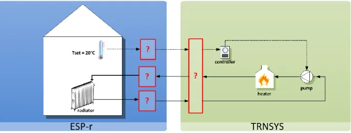
The role of the Harmonizer is to control the coupling, determine the convergence, manage the marching through time of the two programs, and ensure the synchronization of the data exchange. As shown in Figure 2-13, all information exchange passes through the harmonizer. There are no direct data transfer between TRNSYS and ESP-r.
Figure 2-13 Data flows between the Harmonizer and the coupled programs