Evaluation of Demand Forecast Models for Urban Carsharing

POLYTECHNIQUE MONTRÉAL

affiliée à l’Université de Montréal

Evaluation of Demand Forecast Models

for Urban Carsharing

ELHAM KARIMI

Départment de mathématiques et de génie industriel

Mémoire présenté en vue de l’obtention du diplôme de Maîtrise ès sciences appliquées Génie industriel

Avril 2019

POLYTECHNIQUE MONTRÉAL

affiliée à l’Université de Montréal

Ce mémoire intitulé :

Evaluation of Demand Forecast Models

for Urban Carsharing

présenté par Elham KARIMI

en vue de l’obtention du diplôme de Maîtrise ès sciences appliquées a été dûment accepté par le jury d’examen constitué de :

Jean-Marc FRAYRET, président

Martin TRÉPANIER, membre et directeur de recherche Vahid PARTOVI NIA, membre et codirecteur de recherche Francesco CIARI, membre

DEDICATION

This thesis is dedicated to my father: Reza Karimi, my mother: Mehri Pourmand, and my husband: Mahmoud Ramin.

ACKNOWLEDGEMENTS

I would like to express my deepest gratitude to my supervisor, Dr. Martin Trépanier who contributed to my project from the beginning to the end. He inspired me with his kindly continuous financial and spiritual support, knowledge and passion. It would not have been possible without his guidance and constantly availability throughout my research.

I would like to express my gratitude to my co-supervisor, Dr.Vahid Partovi Nia, for his great ideas, knowledge and taking part in this work despite his busy schedule. It was a great pleasure to know him and learn from his invaluable suggestions throughout my whole studies.

Financial support of this work was provided by Communauto carsharing operators. I am grateful for giving me the opportunity to do my master’s thesis. Without their trust this project would be impossible.

I am grateful to Dr. Mina Mirshahi for proofreading different parts of this thesis.

Most importantly, my deepest gratitude goes to my parents, Reza and Mehri, and my brothers for all their unconditional love, engagements, dedications and support from miles away.

Last but definitely not the least, I would like to express my deepest gratitude and appreciation to my lovely husband, Mahmoud, for unconditional love and support. I am indebted to him every bit of success. He is the most important motivation for me to move forward and reach to my dreams.

RÉSUMÉ

Au cours des dernières décennies, les services de mobilité partagée ont été créés en tant que nouvelles alternatives de transport urbain. Le système d'autopartage est l'un de ces services récents impliquant une flotte de véhicules dispersés dans une ville. Cela a permis de contrecarrer certains problèmes, tels que le stationnement limité dans les zones denses de la ville, la pollution, l’augmentation de la possession automobile, etc. Communauto est l’un des plus anciens services d’auto-partage en Amérique du Nord, établi depuis 1994 au Canada.

Le but de ce mémoire est d’appliquer les méthodes d’apprentissage automatique les plus courantes afin de prévoir les heures et les kilomètres consommés selon les réponses souhaitées sur le système opérateur de Communauto avec deux services urbains à Montréal : régulier et en libre-service. La combinaison de différents modèles statistiques et de réseaux de neurones artificiels a été évaluée par le biais d’un ensemble d’expériences afin de prévoir la demande à partir de données historiques. Les modèles appliqués mettent l'accent sur la mise en œuvre de régressions multiples, d'arbres de régression, de forêts aléatoires, de gradient boosting, et des réseaux neuronaux récurrents basés sur long short-term memory et les gated recurrent unit.

Les modèles ont été appliqués aux données de Communauto Montréal. Par la suite des données supplémentaires, telles que les informations sur les journées de vacances et les conditions météorologiques, ont été associées aux données de Communauto Montréal afin de déterminer si les performances des modèles de prévision sont améliorées. Il est à noter que les données relatives au service régulier et aux heures consommées, en tant que réponse, ont été prises en compte pour le processus de prévision.

Les modèles ont été évalués par l’erreur quadratique moyenne sous forme d’indice de mesure de distance entre les valeurs réelles et les valeurs prédites sur la base des ensembles de test. Les ensembles de tests ont été examinés séparément dans les délais suivants : 2012, 2013, 2014 et 2015 à 2016. La moyenne des résultats a ensuite été considérée comme l'erreur finale de chaque modèle. Les résultats montrent que les modèles statistiques tels que l’intensification du gradient en service régulier par rapport au nombre d’heures consommées (avec un taux d’erreur = 1437,48) étaient supérieurs aux modèles de réseaux neuronaux artificiels (taux d’erreur de LSTM = 2159,05, taux d’erreur de GRU = 2215,14). De plus, des facteurs supplémentaires ont amélioré la capacité des modèles de prévision, le taux d'erreur de renforcement du gradient ayant été considérablement

réduit à 1211,96. De plus, les résultats des modèles de prévision en service flottant en ce qui concerne le nombre d'heures consommées et le kilométrage montrent que la régression multiple surpasse les modèles de réseau neuronal artificiel. En outre, les facteurs supplémentaires ont considérablement amélioré les performances des modèles appliqués.

ABSTRACT

In the last few decades, shared mobility services have been made as new urban transport alternatives. Carsharing system is one of these recent services that involves a fleet of scattered vehicles in a city. This helped to counteract some problems, such as limited parking within city in dense areas, pollution, increase in car ownership, etc. Communauto is one of the oldest carsharing services in North America which has been established since 1994 in Canada.

The focus of this thesis is to apply the most common machine learning methods in order to forecast consumed hours and kilometers driven or mileage as desired responses at Communauto operator system with two urban services in Montreal: regular and free-floating. Combination of different statistical and artificial neural network models were evaluated through a set of experiments in order to forecast demand from historical data. The applied models include multiple regression, regression tree, random forests, gradient boosting, long short-term memory and gated recurrent unit based recurrent neural networks.

The models were applied to the Montreal Communauto data. Thereafter, additional factors such as holiday information and weather condition were engaged to the Communauto data to explore whether the performance of forecasting models was enhanced. It is noteworthy that the data related to regular service and consumed hours, as response, were considered for the forecasting process. The models were evaluated by root mean squared error as an index of distance measurement between real and predicted values based on test sets. The test sets were considered separately in the following time frames: 2012, 2013, 2014, and from 2015 to 2016. The average of results was then considered as the final error of each model.

The results show that statistical models such as gradient boosting in regular service with respect to consumed hours (with error rate= 1437.48) outperformed artificial neural network models (error rate of LSTM = 2159.05, error rate of GRUs = 2215.14). Moreover, additional factors improved the ability of the forecasting models, as the error rate of gradient boosting was significantly reduced to 1211.96. Furthermore, the results of forecasting models in free-floating service with respect to consumed hours and mileage show that multiple regression outperformed artificial neural network models. Besides, the additional factors significantly improved performance of the applied models.

TABLE OF CONTENTS

DEDICATION ... iii

ACKNOWLEDGEMENTS ... iv

RÉSUMÉ ... v

ABSTRACT ...vii

TABLE OF CONTENTS ... viii

LIST OF TABLES... xi

LIST OF FIGURES ...xii

LIST OF SYMBOLS AND ABBREVIATIONS ... xiv

LIST OF APPENDICES ... xv CHAPTER 1 INTRODUCTION ... 1 1.1 Background ... 1 1.2 Research Project ... 3 1.3 Research Objectives ... 4 1.4 Thesis Structure... 5

CHAPTER 2 LITERATURE REVIEW ... 8

2.1 Carsharing System ... 8

2.2 Supervised Machine Learning Algorithms ... 9

2.2.1 Multiple Regression ... 10

2.2.2 Regression Tree ... 11

2.2.3 Random Forests ... 12

2.2.4 Gradient Boosting ... 12

2.2.6 GRUs Recurrent Neural Networks ... 14 2.3 Performance Metrics ... 14 CHAPTER 3 METHODOLOGY ... 15 3.1 Problem Review ... 16 3.2 Data Description ... 16 3.2.1 Communauto Dataset ... 16 3.2.2 Weather Dataset ... 20 3.2.3 Holiday Dataset ... 21 3.3 Data Preprocessing ... 21 3.3.1 Null Values ... 21

3.3.2 Detecting Outlier: BOX Plot Diagram ... 22

3.3.3 Encode Categorical Variables ... 22

3.3.4 Normalized Data ... 23

3.3.5 Data Visualization ... 23

3.4 Data Splitting: Forward-Chaining ... 24

3.5 Data Modeling ... 24

3.5.1 Multiple Regression ... 25

3.5.2 Regression Tree ... 27

3.5.3 Random Forests ... 29

3.5.4 Gradient Boosting ... 30

3.5.5 Recurrent Neural Networks ... 30

3.6 Evaluation Methods... 34

CHAPTER 4 IMPLIMENTAION AND RESULTS ... 35

4.1.1 Remove Null Values... 36

4.1.2 Discard Outliers by BOX Plot Diagram ... 36

4.1.3 Convert Categorical Variables to Dummy Variables ... 38

4.1.4 Test Samples ... 39

4.1.5 Data Visualization ... 40

4.2 Experiments ... 46

4.2.1 Experiment 1 : Multiple Regression ... 47

4.2.2 Experiment 2: Regression Tree ... 49

4.2.3 Experiment 3: Random Forests ... 50

4.2.4 Experiment 4: Gradient Boosting ... 52

4.2.5 Experiment 5: Long-Short Term Memory RNNs ... 53

4.2.6 Gated Recurrent Units RNNs ... 55

4.3 Evaluating Forecasting Models... 57

CHAPTER 5 CONCLUSION AND RECOMMENDATIONS ... 63

5.1 Regular Service ... 64 5.2 Free-floating Service ... 64 5.3 Future Directions ... 64 BIBLIOGRAPHY ... 66 APPENDICES ... 68

LIST OF TABLES

Table 3-1: Description of Communauto dataset ... 18

Table 3-2: Description of the most relevant variables of Communauto dataset ... 20

Table 4-1: Descriptive statistics of numeric variables in REG (regular service) dataset ... 38

Table 4-2: The experiment results obtained from forecasting models by using REG data ... 58

Table 4-3: The experiment results obtained from forecasting models by using REG data combined with holiday and weather data ... 60

LIST OF FIGURES

Figure 1-1: Communauto operating distribution in real-time status map in Montreal

(Communauto Inc, 2019). The orange pins indicate available automobiles in free-floating

service. The green pins show the active stations in regular service. ... 2

Figure 1-2: Example trend of consumed hours during a year in regular service of Communauto operation. ... 4

Figure 1-3: Thesis outline ... 6

Figure 3-1: The design summary for forecasting process ... 15

Figure 3-2: A recursive partitioning tree ... 28

Figure 3-3: Architecture of Long Short-Term Memory unit (Witten et al., 2016) ... 31

Figure 3-4: Sigmoid activation function (Abhijit Mondal, 2017) ... 32

Figure 3-5: Architecture of Gated Recurrent Units (Danny Mathew, 2018) ... 33

Figure 4-1: Box plot to illustrate the distribution of a kilometer per hour. The lower and upper quartiles and lower and upper limits from the obtained feature (compare) are marked. Moreover, the outliers are shown by red arrow. ... 37

Figure 4-2: Split data to four folds as training and test sets. ... 39

Figure 4-3: Distribution of single variable and scatter plots to show the relationship between variables (REG dataset)... 41

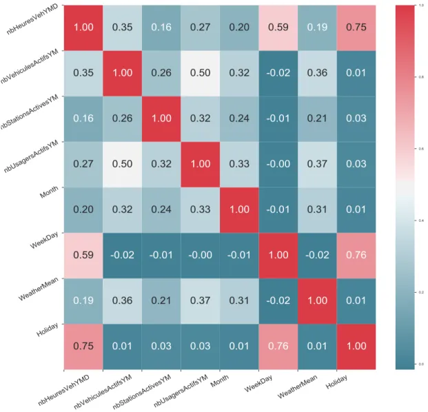
Figure 4-4: Correlation matrix between variables (REG dataset) ... 42

Figure 4-5: Box plots of consumed hours by day of week (REG dataset) ... 43

Figure 4-6: Box plots of consumed hours by holiday time (REG dataset) ... 44

Figure 4-7: Box plots of consumed hours by month (REG dataset) ... 45

Figure 4-8: Box plots of consumed hours by weather conditions (REG dataset) ... 46

Figure 4-9: Left: The plot of real values vs. predicted values in multiple regression model by REG data. Right: The plot of real values vs. predicted values in the same model by REG data, holiday and weather dataset. ... 49

Figure 4-10: Left: The plot of real values vs. predicted values in multiple regression model by REG data. Right: The plot of real values vs. predicted values in the same model by REG data, holiday and weather dataset. ... 50

Figure 4-11: Left: The plot of real values vs. predicted values in multiple regression model by REG data. Right: The plot of real values vs. predicted values in the same model by REG data, holiday and weather dataset. ... 51 Figure 4-12: Left: Bar chart of importance variable in random forests model with REG data.

Right: Bar chart of importance variable in random forests model with REG data and additive features. ... 52 Figure 4-13: Left: The plot of real values vs. predicted values in multiple regression model by

REG data. Right: The plot of real values vs. predicted values in the same model by REG data, holiday and weather dataset. ... 53 Figure 4-14: History plot of loss function... 54 Figure 4-15: Left: The plot of real values vs. predicted values in multiple regression model by

REG data. Right: The plot of real values vs. predicted values in the same model by REG data, holiday and weather dataset. ... 55 Figure 4-16: History plot of loss function... 56 Figure 4-17: Left: The plot of real values vs. predicted values in multiple regression model by

REG data. Right: The plot of real values vs. predicted values in the same model by REG data, holiday and weather dataset. ... 57 Figure 4-18: Comparison of the error measurement RMSE of models on REG data by

box-whisker plot. ... 59 Figure 4-19: Comparison of the error measurement RMSE of models on REG data combined

LIST OF SYMBOLS AND ABBREVIATIONS

AIC Akaike Information Criterion ANNs Artificial Neural Networks AUM Auto-Mobile Service

BIC Bayesian Information Criterion CSV Comma Separated Values GRUs Gated Recurrent Units IQR Interquartile

LSTM Long Short-Term Memory MSE Mean Squared Error

Q Quartile

REG Regular Service

RMSE Root Mean Squared Error RNNs Recurrent Neural Networks Tanh Hyperbolic Tangent

LIST OF APPENDICES

Appendix A- The results of multiple regression on “REG” data ... 70 Appendix B- Experiment results overview on “REG” dataset respected to mileage ... 74 Appendix C- “AUM” dataset (free-floating service) respected to consumed hours and mileage . 75

CHAPTER 1

INTRODUCTION

1.1 Background

Over the years, carsharing services as an alternative to private vehicles with the ability to share cars with other users have gained significant traction. Members of carsharing services have access to a fleet of scattered vehicles without owning them. In this sense, users can take advantage of using vehicles privately regardless of the concerns expressed by the lease payments, insurance, gas filling, maintenance or parking. Therefore, cost effectiveness and accessibility are the main incentives for joining as a user of carsharing operators. Carsharing services have been developed and they have turned into one of an important and efficient element in moving passengers in local and suburban areas (Murray, Davis, Stimson, & Ferreira, 1998). More importantly, carsharing program as a modern approach has had a massive impact on environmental and transportation issues (Katzev, 2003). Therefore, the program has been extremely prosperous worldwide. Considering this fact, a lot of agencies have been fascinated by this kind of transportation, showing that the number of carsharing programs has been expanding around the world (Shaheen & Cohen, 2007).

Communauto is a carsharing organization pioneer based in Montreal, Canada, which has been one of the oldest and fastest enlarging carsharing services since 1994 in North America. Communauto carsharing services have been available in several cities in Quebec province of Canada, including Montreal, Quebec City, Sherbrooke, and Gatineau. In addition, carsharing services have been supplied by this organization under the name of VRTUCAR in the province of Ontario and Nova Scotia. Moreover, it has recently been developed in capital of France, Paris, and the suburbs. Fleeting car rental which has been promoted by this organization is comprised of 2 packages: regular and free-floating services. Regular carsharing operation,sometimes called round-trip, is developed with station-based systems by-which cars should be returned to the same dedicated station where users pick up. Travelers are charged for each kilometer and hour on every journey. Free-floating operator which offers Auto-Mobile vehicles, is planned to be one-way and is dispersed aboard specified zones without stations. Hence, this model in contrast to regular service allows users to take vehicles and drop off cars at any convenient on-street space within the legal zone. The term of this service is based on per minute fare. In both services, registered users can make a request to reserve available cars online or through smartphone applications. However, for

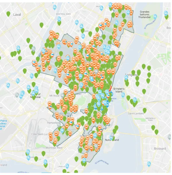
free-floating, the reservation window is 30 minutes, which is much smaller than for the regular service, in-which cars can be reserved up to 30 days ahead. Figure 1.1-1 shows a distributed fleet of vehicles at different locations in Montreal.

Figure 1-1: Communauto operating distribution in real-time status map in Montreal

(Communauto Inc, 2019). The orange pins indicate available automobiles in free-floating service. The green pins show the active stations in regular service.

In the last few years, the sizeable applicants have become more mindful to join Communauto carsharing networks. Therefore, the ratio of members has been drastically rising. Due to changes in demand and impressive growth of members, carsharing operators have faced complex challenges

of restrictions on supply. In the light of this situation, the operation efficiency of this system relies on recognition of users' demands, and the benefit which will assist the company's survival for serving their services. Discovering about usage patterns must be an essential element to overcome restrictions and quick progress of the company.

Technology advancements have allowed generating data day-to-day. The collected data in this project are integrated by tracking the daily trips of users along with more details such as consumed hours and driven kilometers. Additionally, the agency's facilities include the number of active stations (for regular service) and available vehicles.

Machine learning methods are available in building accurate forecasting models and recognizing trends or patterns as they could emphasize a significant impact on the quality of the system. However, traditional methods may be more accurate in some applications, and it is relevant to examine different models to see their forecasting performance.

1.2 Research Project

The main focus of this thesis is developing methods aimed to forecast the demand of carsharing service, then assess the tuned models and their performance. The demand values of regular and free-floating services are defined as 1) consumed hours and 2) mileage (km). Indeed, the task is to forecast the future demand given series of historical observations, and moreover, investigating the factors affecting vehicle usage in Communauto carsharing operator, such as holiday and weather conditions, to be taken into optimizing the ability of the models.

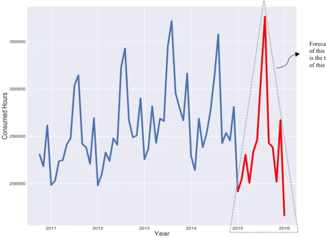
Figure 1-2: Example trend of consumed hours during a year in regular service of Communauto operation.

For example, Figure 1.2 shows the overall trend of consumed hours as one of the demands of this thesis. The blue colored observations are used to train the machine learning algorithms. The target is to forecast the red colored part.

1.3 Research Objectives

Apart from developing a demand forecasting model, the specific objectives of this work are to determine whether the forecasting power of the “traditional” statistical models outperform that of artificial neural networks models.

In order to explore the goal of the research, the following experiments are performed:

• Visualizing the dataset to detect data quality issues such as outliers, then perform cleaning.

Forecasting of this part is the target of this study

• Exploring and seeking strong patterns and regularities between independent variables which are referred to features in this thesis.

• Applying forecasting models such as multiple regression, regression tree, random forests, gradient boosting, long short-term memory (LSTM) recurrent neural networks and gated recurrent units (GRUs) based on recurrent neural networks (RNNs) algorithms.

• Training the model on different samples of the data.

• Evaluating the models and comparing the models' performance

The forecasting models would be beneficial for the Communauto operation in order to forecast consumed hours and mileage as our dependent variables in this research. The results can undoubtedly assist the company to enhance further facilities to the existing members, thereby better expand their services in upcoming years. Moreover, this study will assist in better understanding of the demand for vehicles in the Communauto carsharing network.

1.4 Thesis Structure

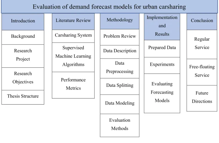
The layout of the current study is organized as shown in Figure 1.3, with 5 chapters in total. Each chapter is separated into different sections:

Figure 1-3: Thesis outline

• Chapter 2 (Literature Review) gives an overview of carsharing systems. Moreover, this chapter is conducted to reach an insight into machine-learning algorithms and the related work in supervised learning models such as multiple regression, regression tree, random forests, gradient boosting, LSTM and GRUs recurrent neural networks. Then, performance metrics are discussed in this part.

• Chapter 3 (Methodology) introduces several enriched datasets under this study. Then, relevant features, which contribute most to forecast outputs or responses in which this thesis is interested in, are extracted. Moreover, data pre-processing and visualization of data is done before applying the intended supervised techniques. Then, the methods which are used to create forecasting models are explained in detail. Finally, evaluation methods are introduced in this chapter.

• Chapter 4 (Results) implements the methods which are introduced in chapter 3 to clean the data from the noisy points and missing values. Afterward, the prepared data is used to learn the forecasting models such as multiple regression, regression tree, random forests, gradient

Introduction Background Research Project Research Objectives Thesis Structure Literature Review Carsharing System Supervised Machine Learning Algorithms Performance Metrics Implementation and Results Prepared Data Experiments Evaluating Forecasting Models Conclusion Regular Service Free-floating Service Future Directions Methodology Problem Review Data Description Data Preprocessing Data Splitting Data Modeling Evaluation Methods

boosting, LSTM and GRUs recurrent neural networks. Finally, the performance of each model is evaluated using the root mean squared error (RMSE).

• Chapter 5 (Conclusion) discusses the results of the forecasting models on Communauto dataset with and without holiday and weather variables as additive features, as well as further research in the field.

CHAPTER 2

LITERATURE REVIEW

This chapter gives an insight provided on what the pertinent work is done in the field of carsharing systems and supervised machine learning algorithms. The review is widely arranged into three discussions. In section 2.1, the general background about carsharing services is described. Subsequently, the application and information about supervised machine learning models in forecasting are given in section 2.2. The discussion is regarding previous work done by modeling algorithms such as multiple regression, regression tree, random forests, gradient boosting, LSTM and GRUs recurrent neural networks which are ensemble machine learning models. In addition, section 2.3 provides the reflection of evaluating the models and method selection.

2.1 Carsharing System

While the world population has experienced rapid growth, transportation systems boast a remarkable role in economic satisfaction impacts, improve levels of life quality, however, causing excessive automotive mobility and threatening the environmental sustainability.

Shared mobility refers to transportation services that are shared among users which is nowadays used very broadly. It is including public transit, taxi, bike sharing, carsharing and other transportation modes.

Since the mid-1980s, carsharing systems as an easily accessible tool, have become popularized gradually across the world (Murray et al., 1998). The concept of carsharing is based on that the number of needed cars to provide the demand of members are dramatically less than when each user owns privet vehicles. Carsharing service provides users with access to shared vehicles for usually short-term use. The shared vehicles are scattered within a network of locations in a city. Carsharing creates the possibility to access a car at any time with a reservation, and the users are charged by either time or mileage. Round-trip and one-way are the most common models of carsharing operation. In both models, the fleet of vehicles are used for several trips by multiple users throughout the day. In round-trip, vehicles must be returned to the same location where users borrow the car. However, one-way system allows customers to take a vehicle at one location and drop it off at the other location.

This type of transportation mode helps to reduce car ownership with the growing access to use a shared fleet of vehicles which is more affordable than owning a personal car. Additionally, studies by Steininger and colleagues have shown that most European carsharing users do not own a car

(Steininger, Vogl, & Zettl, 1996). In this sense, users can take advantage of using shared vehicles regardless of the concerns about wasting time to rent a car from agencies and getting charged for the full day. In fact, users can reserve cars online or by smartphone applications prior to using them. Moreover, vehicles can be picked up at the nearest specified zones or stations with tolerable walking. Shared fleet organizations are responsible for paying all expenses of vehicle maintenance and repairs. Meanwhile, parking and insurance coverage are provided through them. So far, carsharing has had a significant effect on reducing vehicle ownership around the world. For instance, in 2001, B. Robert, the founder of Communauto in Canada, reported that 25% of the members of this organization sold their vehicles and more than 50% were able to avoid buying a car (Katzev, 2003).

In late 1994, Communauto was launched as one of the largest commercial organizations in North America, based in Montreal, Quebec. Most of its stations and zones are placed within residential areas, although some are located in central business areas or near transit nodes. Travellers are charged by the time and mileage which depends on the type of services that they use.

Obviously, Communauto carsharing service in Montreal has taken a major contributor to a mode of transportation along with low-pollutant emission vehicles. Moreover, Sioui et al. conducted a study on Communauto members which shows that most users who do not have private vehicles and often use carsharing services, drive 30 percent less than those who own private vehicles (Sioui, Morency, & Trépanier, 2013). Insofar as a study on carsharing systems is described by Martin and Shaheen, it presents a significant decrease in vehicle-kilometers driven after joining carsharing systems, although the drivers had their personal vehicles (Martin & Shaheen, 2011). Another positive effect which is assessed by the same researchers is the reduction of greenhouse gas emission in Canada and the US.

2.2 Supervised Machine Learning Algorithms

In the last 20 years, machine learning algorithms have been evolved as an important foundation of information technology. Machine learning algorithms are drastically applied with a variety of approaches in different problems which let computers exploit information by observing raw data and extracting patterns, then analyzing and optimizing performances (Witten, Frank, Hall, & Pal, 2016). This knowledge is remarkably applicable in high-level of computing (Y. Chen et al., 2014). Machine learning, a subfield of computer science, has generated a revolution in statistical science.

The expression of learning comes up with improvement of algorithms with respect to past experience and gained knowledge (Das & Behera, 2017).

In computer science, an algorithm is a set of instructions in order to express operations to find the most efficient way of carrying out response process of the object. In machine learning, algorithms are used to design mathematical models in order to produce informative results or uncover reliable associations hidden within observations (Alpaydin, 2009). Ongoing research and daily activities interact directly with machine learning, including weather forecasting, managing transportation, pattern recognition, fraud detection, medical diagnosis, and many other complex analytic purposes. Understanding the data is critical in order to recognize and implement various methodologies with more efficiency. In this setting, depending on existing data, most machine learning algorithms are broadly characterized into one of two categories: supervised learning and unsupervised learning. Supervised learning is focused on the samples where data has been labeled, and input and response are known. Indeed, this type of data allows a system to extract the hidden structure of data and builds the robust forecasting of unseen or test data (Mohri, Talwalkar, & Rostamizadeh, 2012). On the other hand, the data without labels are elaborated as unsupervised learning or clustering techniques. Whereas, in no ascribe labels on data, the learner detects the similarities between points, and then spreads them into various categories. Accordingly, each category takes the new label (Hastie, Tibshirani, & Friedman, 2009).

Some supervised learning models are proclaimed to overcome noisy data or overfitting issues to make a robust model. On the other hand, some models are interpretable and low flexible, while others are non-interpretable and highly flexible (Lipton, 2016). Practitioners should ask which models are matched to task and available dataset. In the following section, a detailed review of the concept and previous studies of applied models like multiple regression, regression tree, random forests, gradient boosting, RNNs with LSTM and GRU units are considered.

2.2.1 Multiple Regression

The initial form of regression (least squares) was published in early nineteenth century by Legendre and Guass, and the term of regression was later expressed by Francis Galton (Bingham, 2006). Regression as a statistical measurement is used to determine the relationship between dependent and independent variables. Moreover, it is widely employed to fit a forecasting model. Many techniques have been developed for carrying out regression analysis.

Multiple regression is a statistical approach utilized for modeling with more than one independent variable or feature (Osborne, 2000). The correlation between variables is examined in this model to screen out the effect of each independent variable on the dependent variable or response, and to describe what variables have conceptual senses in a forecasting. Moreover, interaction effect is a common phenomenon in regression analysis, when the interaction of one or more independent variables have a high influence on the performance of the model and forecasting the response value. Hence, in most problems, interaction terms are significant in statistical concepts and modeling (James, Witten, Hastie, & Tibshirani, 2013).

In 1982, Bean proposed a powerful multiple regression model for forecasting student behavior by deploying the interaction term (Bean, 1982). Later on, in 1986 Smouse and colleagues employed an efficient forecasting model with the mentioned method in biology research (Smouse, Long, & Sokal, 1986). It is widely acknowledged that weather forecasting and seasonal climate assessment (Krishnamurti et al., 1999), bike rental demand (Ji, Cherry, Han, & Jordan, 2014), brain research (Klein, Foerster, Hartnegg, & Fischer, 2005), and more scopes are feasible through multiple regression along with the strong forecasting results.

2.2.2 Regression Tree

In recent years, most of the research in statistical learning has been located on non-linear methods. However, non-linear methods often have drawbacks such as low interpretability power in comparison with linear models, but they are adept in discovering pertinent interaction among variables and accurate results (James et al., 2013).

Within most research efforts, decision tree and regression tree have become popular as tree-fitting models (Breiman, Friedman, Olshen, & Stone, 1984). Decision tree is used when the dependent variable is categorical, which is out of the scope of this study. Regression tree can accommodate continuous dependent variables. Since 1991, regression tree has been started up as a powerful model in forecasting problems (Karalic & Cestnik, 1991).

Briefly, tree-based regression is grown by applying greedy algorithms to speedy split that recursively partitions the training set into successively tiny subgroups (Kohavi & Quinlan, 2002). Consecutively, splits are examined for all independent variables, and ultimately the best submission is considered by measuring the impurity by indicating homogeneity in the lower level of the tree.

Augustin and his crew showed that regression tree is able to evaluate risk forecasting in medical scope as an alternative to various models by presenting accurate forecast models (Augustin et al., 2009). The results coming from recent successes show that regression tree, despite its shortcomings, still has special popularity among ecological researchers for exploring interaction and pattern recognition (De'ath & Fabricius, 2000).

2.2.3 Random Forests

Random forests methodology is known as one of the impressive learning models. This method was proposed by Breiman in 1984 which can be used to fit forecasting models for regression and classification problems. An early technique is called bagging which was introduced by Breiman in 1996 and it is a general approach that can be applied in many machine learning methods. Bagging is a method for creating multiple version sets from training set and it helps to improve the model by using each of the sets for training the model (Breiman, 1996). Therefore, bagging contains several trees which most or all deploy the stronger feature in the top split. Breiman has shown another technique in 2001 which only considers a subset of the features for each split. Hence, in all trees the strong feature is not only considered feature, while other features have chance to be in the top split (Breiman, 2001).

Random forests are used in many fields in order to make a robust forecasting model which outperforms artificial neural networks model (Palmer, O'Boyle, Glen, & Mitchell, 2007).

2.2.4 Gradient Boosting,

Gradient boosting is one of the fundamental advances in statistical tools with high adaptability along with elegance and simplicity, which is applicable for both regression and classification for a vast scope of problems and various supervised learning models (Friedman, 2001). This method led to understanding and tuning of model's parameters which can be used to attain the best forecasting model (Kuhn & Johnson, 2013). Due to its numerous benefits, researchers and developers such as Gilberto Titericz, have become a fan of gradient boosting who previously were eager to neural networks. Persson development team drove gradient boosting as an efficient machine learning model in a multi-site framework for fitting a forecasting model of future power generation in Japan (Persson, Bacher, Shiga, & Madsen, 2017). Performance models were evaluated in comparison

with benchmark models; thereby, the results showed that gradient boosting surpassed other models. Robustness and flexibility as criteria were also considered.

2.2.5 LSTM Recurrent Neural Networks

Artificial neural networks (ANNs), as alternative methods of statistical approaches, have drawn substantial consideration in variant scopes, containing computer science, statistics, business, and even diagnosis or treatment. The initial development was inspired by the human brain's neural format, which generate and explore new models in learning (Zhang, Patuwo, & Hu, 1998). ANNs are scattered as one of the major efficient forecasting approaches in several applications. Lapedes and Farber were a pioneer in developing forecasting applications of ANNs (Lapedes & Farber, 1987). In this knowledge, various architectures have been expanded with different neurons arrangement. The long short-term memory based on recurrent neural network is most widely for sequential dataset.

Recurrent Neural Networks are popular networks that have proposed supreme premise in major tasks. In particular, the mentioned model is accommodated with historical, sequential and even time series datasets. RNNs as an extension of neural networks are also based on the premise that the networks handle consecutive information and the connection forms which are in oriented cycles state (Witten et al., 2016). The term of Recurrent in RRNs implies implementing the same role for every member of a sequence, and the extracted result depends on the prior actions. This situation in RNNs proves the memory simply in this model, which retains informative results in each period (Chung, Gulcehre, Cho, & Bengio, 2014). Although, Bengio et al. realized that RNNs are not able to hold informative asset in long-term which impresses negative effect on model performance (Bengio, Simard, & Frasconi, 1994).

Researchers struggled for a while to overcome this weakness and gain an effective execution. Hochreiter and Schmidhuber designed LSTM to enhance the capability of RNNs for learning in long-range dependency (Hochreiter & Schmidhuber, 1997). Lately, Kang and Chen employed LSTM recurrent neural networks for forecasting traffic streams, and yielded significant achievements (Kang, Lv, & Chen, 2017). Recognizing a temporal pattern of traffic is indispensable for the transportation system, because undoubtedly the obtained forecasting models and results could inspire urban development.

2.2.6 GRUs Recurrent Neural Networks

GRUs as a new version of LSTM is recently provided by Cho et al. (Cho, Van Merriënboer, Bahdanau, & Bengio, 2014).GRUs address problems similar to LSTM with low memory demand. It technically means that there is no necessity to employ detached memory cells in process of capturing information inside units. Therefore, considering low-cells in described model led up to more efficiency than LSTM. Note that GRU is plainer and more computational than LSTM (Chung et al., 2014). In 2017, Chen et al. demonstrated that recurrent neural networks with GRU blocks, can be applied in order to fit a model to forecast bike demands with concern about distribution of bikes in sharing service. The proposed model in this study was compatible with time series dataset (P.-C. Chen, Hsieh, Sigalingging, Chen, & Leu, 2017).

2.3 Performance Metrics

Fitting a model for forecasting future data is one of the steps of forecasting process. The next step is measuring the quality of the model. In order to assess the desirability of machine learning algorithms on a determined dataset, performance metrics assist to measure models' quality to fit in accordance with observed data. Furthermore, these metrics are highly substantial for evaluating and comparing different algorithms to each other based on various criteria such as stability, robustness to noise and so more, which depend on the type of problem. For instance, in regression models, mean squared error (MSE) is usually used, given by:

MSE = _'& ∑' (𝑦₊ − 𝑦-₊)/

+0& (2.1)

where 𝑦₊ is referred to actual value for given data, and 𝑦-₊ is the value returned by the model or predicted value. In equation (2.1), training data is used for generating the model, and test data is applied to examine the model with-which difference is adverted to the accuracy of predicted model. Due to the model variety, decision for selecting the best metric for the model assessment is usually not easy. Some of the other statistical tools for measuring the goodness of the result are as following: root mean squared error (RMSE), adjusted 𝑅/_{, Akaike information criterion (AIC),} Bayesian information criterion (BIC), Mallow's 𝐶₃, and more. Each of them is adjusted to judge specified methods and issues (James et al., 2013)

CHAPTER 3

METHODOLOGY

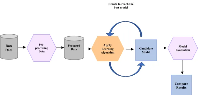
The proposed methodology is explained in this chapter. Section 3.1 discusses about the goal of this thesis. Section 3.2 introduces the types of dataset, consisting of Communauto, holidays and weather dataset in CSV format. This section also covers selection of the most relevant variables with the considered responses, individually for each dataset. Thereafter, section 3.3 represents the foremost practice step to visualize given data in order to clean and prepare the raw data for analyzing, by using Python language programming. Data splitting and its effect on performance of a model are described in section 3.4. Section 3.5 is about adopting some machine learning techniques which are used in this project. The learning procedure is explained by how candidate models can be practically applied to the dataset to uncover patterns. Moreover, in section 3.6, performance of the techniques is evaluated through test or validation set to forecast desired response (consumed hours and mileage). The summary of the processes of this study is shown in Figure 3.1.

Figure 3-1: The design summary for forecasting process Raw Data Pre-processing Data Prepared Data Candidate Model Model Evaluation Compare Results

Iterate to reach the best model

Apply

Learning Algorithm

3.1 Problem Review

The main goal of this thesis is to build some forecasting models by supervised machine learning techniques, based on the historical dataset. This project is carried out as a comparative analysis for forecasting algorithms. The principal concern of this study is forecasting the consumed hours and mileage as desired responses or outputs of this study regarding to different factors. Initially, the model will be built without involving additive factors, thereafter, they will be engaged to investigate whether they improve the performance of the models or not.

Principally, in order to have the best model with lowest error rate, some operations should be employed to prepare the data, take the informative variables, and build a model.

3.2 Data Description

In order to interrogate the factors affecting consumed hours and mileage in the Communauto carsharing system as the targets of this research, three different sources of data are applied to serve. Applied data includes: (1) Communauto carsharing services, (2) historical weather conditions in Montreal and (3) holiday information of Quebec Province. The following sections are provided to explain every sample in detail with different features and several types of values. Moreover, data preparation procedures such as feature dropping or variables augmentation are presented in each data description. It is noteworthy that the pertinent datasets to regular and free-floating services are subcategorized under Communauto dataset section.

3.2.1 Communauto Dataset

These datasets have been provided by Communauto carsharing network based in Montreal. As mentioned in the first chapter, this company has been providing regular or station-based, and free-floating (called “Auto-Mobile”) services. The dataset is gathered by both services that can be distinguished through the column assigned to service. It means that accumulated rows by AUM in the column labeled as service refer to the free-floating “Auto-Mobile” service, and the other part which is displayed by REG is related to the station-based or regular service.

Both services have the same variables as the other one and the only difference is the variable which is dedicated to the number of active stations. There is no station in free-floating service because the users take the fleet of scattered vehicles which are available in the authorized zone.

The given dataset brings CSV (comma-separated values) file of carsharing trip histories, which consists of 2982 observations with 10 variables. The recorded information in Communauto dataset contains the number of stations, vehicles, users, reserved and free cars, and total consumed hours and mileage on each day which are conducted from 2010 to 2016 for regular service and 2013 to 2016 for free-floating service.

Each variable is typically called “feature” in this thesis. As previously mentioned, the main goal of this project is forecasting the consumed hours and mileage in the company of interest. Therefore, the variable labeled by nbHeuresVehYMD (consumed hours) and distTotaleKmReservation (mileage) are considered as individual dependent variables or output which is referred as response in this report.

It should be noted that each response as a target of this research is uniquely placed under the study. Hence, the regular-service or REG dataset and consumed hours, as response, are considered for the forecasting process. The approach is the same for mileage as another target and Auto-Mobile service dataset in this research. The results are demonstrated in this report.

• Feature Importance

The Communauto dataset is decomposed into two particular sets: 1) Auto-Mobile (AUM) 2) regular (REG). The first 1005 rows include AUM observations from 2013 to 2016, and the rest include 1977 rows related to REG information between 2010 and 2016. Table 3.1 illustrates the details of this dataset.

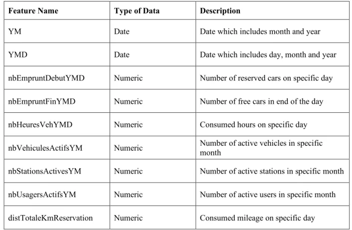
Table 3-1: Description of Communauto dataset

Feature Name Type of Data Description

YM Date Date which includes month and year

YMD Date Date which includes day, month and year

nbEmpruntDebutYMD Numeric Number of reserved cars on specific day

nbEmpruntFinYMD Numeric Number of free cars in end of the day

nbHeuresVehYMD Numeric Consumed hours on specific day

nbVehiculesActifsYM Numeric Number of active vehicles in specific

month

nbStationsActivesYM Numeric Number of active stations in specific month

nbUsagersActifsYM Numeric Number of active users in specific month

distTotaleKmReservation Numeric Consumed mileage on specific day

The principal task is to remove the feature that do not have an influence on this study. To this end, in both of the grouped data, the first feature labeled as YM is eliminated, because the next labeled as YMD represents more detailed aspects of the timestamp information to identify the year, month and day. Due to the YMD feature, observations are the sequence of historical spanning data, since this research is aimed to forecast the desired responses in different month and daytime scale. Therefore, YMD feature in a couple of processing can be isolated into the month and week of day variables. The column including the number of months is determined by values between 0 to 12 in the specified year, where 0 refers to the month of January. The week of day variabel is filled with day types, which are represented by a number between 0 to 6 in weekday observations, in-which Monday is considered as the start day (day 0). The recorded date can assist to answer the following questions: Whether the amount of consumed hours and mileage will be depended on different months, and which months will be more aggregated? What kind of days in this service has the most frequent usage, work day or weekend?

Moreover, none of the variables labeled as nbEmpruntDebutYMD and nbEmpruntFinYMD, referring to number of reserved car and free vehicles at the end of the day, contain effective information about the desired responses under this study. The irrelevant features may significantly degrade the performance of a forecasting model. In such a case, these features can be discarded from the initial dataset without performance deterioration in forecasting process.

The available data related to AUM or Auto-Mobile service has the same features except the variable labeled as nbStationsActivesYM. Notice that all the operation lines above, are applied to preparing the AUM set.

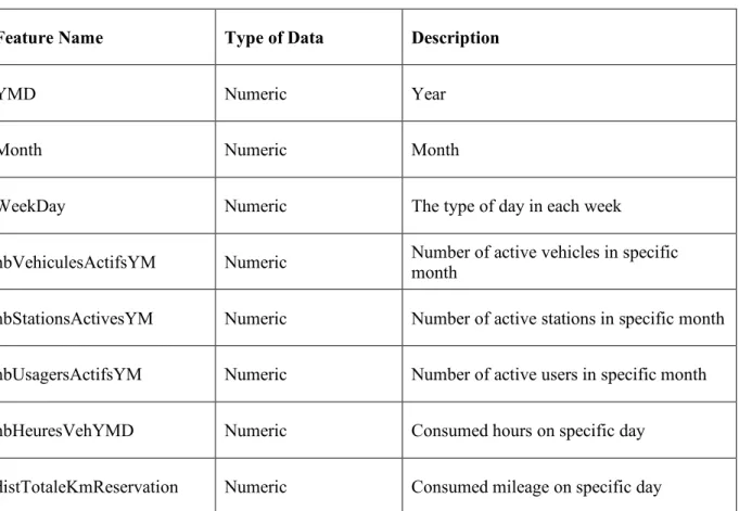
After dropping those features, basically the dataset contains six main features with nature of date, character and number: YMD, Month, WeekDay, nbVehiculesActifsYM, nbStationsActivesYM, and nbUsagersActifsYM. Table 3.2 describes comprehensive information of features and response variables in Communauto dataset.

Table 3-2: Description of the most relevant variables of Communauto dataset

Feature Name Type of Data Description

YMD Numeric Year

Month Numeric Month

WeekDay Numeric The type of day in each week

nbVehiculesActifsYM Numeric Number of active vehicles in specific _month

nbStationsActivesYM Numeric Number of active stations in specific month

nbUsagersActifsYM Numeric Number of active users in specific month

nbHeuresVehYMD Numeric Consumed hours on specific day

distTotaleKmReservation Numeric Consumed mileage on specific day

The considered features interfere with the process of creating forecasting models in order to forecast the consumed hours and mileage in the specified time as the targets of this study.

3.2.2 Weather Dataset

The historical weather dataset represents the overall conditions in Montreal that is recorded in CSV format during the period from January 1, 2008 to December 30, 2017. Each observation is incorporated with daily weather. This dataset is composed of several features, such as maximum, minimum and mean of temperature, the amount of rain and snow during the day and more.

• Feature Importance

The columns pertinent to rain and snow must be ignored, because most of them are filled by null values and do not provide much information. Therefore, to avoid imposing the complexity in analyzing and modeling procedure, the average temperature is considered as a part of data under this study. The varibale labeled WeatherMeannTemp is referred to the average temperature in dataset. The recorded observations in this feature are numeric, which are restricted within the range

between -25 to 30 in Celsius scale. In this case, the values in the column WeatherMeannTemp can be converted to two levels of possible dummy variables, zero and one.

3.2.3 Holiday Dataset

In Canada, holiday depends on the province. Typically, each province has its own holiday periods. The major public holiday information of Quebec province is presented in CSV file between January 1, 2010 to February 31, 2016. Saturday and Sunday are counted as holiday in obtained dataset based on a hypothesis that consumed hours and mileage are different on workday and weekend. Hence, the data model just distinguished between holiday and non-holiday or working days. In two categorized classes, holiday times are shown by Yes and the rest are represented by No.

3.3 Data Preprocessing

Usually, raw data is seldomly suitable for analysis and feeding algorithms. Such data have significant effect on the performance of a model. The preliminary and critical task is to investigate the quality of the given data. Most often, real data is congregated by incomplete, inconvenient, unreliable and distorted information. In order to do this, it is required to clean up the initial data from redundant and irrelevant information. Data preprocessing knowledge covers several tasks with the aim to convert raw data into an applicable format and prepare the data before formal analysis. In fact, preprocessing knowledge trace potentially significant information in initial data, understand the complexities and discover good ways to handle such issues. Generally, data preprocessing would fairly lead to achieving significant performance of supervised models (Kotsiantis, Kanellopoulos, & Pintelas, 2006).

3.3.1 Null Values

Missing or unknown values are an unavoidable problem in raw data and can have a substantial impact on final results. There are varieties of sources to implicate the data into issues such as mistakes in measurements, misrecording of data and so on (Kantardzic, 2011). Available sample received on behalf of Communauto company contains some of the missing observations which are distinguished by 0 and NA. To resolve this issue, because the missing data is restricted to a few cases and the quantity of data is enough for analysis and query, the rows which meet this state are dropped from the dataset (Scheffer, 2002).

3.3.2 Detecting Outlier: Box Plot Diagram

Outlier is as an unusual observation that is stated outside the overall pattern of data model and it is drastically inconsistent with other observations. Such outliers typically have an unpleasant influence on the results made from the study. This issue can arise due to a variety of either faulty recording or empirical error. In other words, outliers are awarded to the observations that the response 𝑦+ is weird given the feature 𝑥+ (Kuhn & Johnson, 2013). These types of unusual values require precise analysis before deciding whether they should be eliminated from the population under study, or not.

Box plot diagram is a convenient method in order to identify outliers and eliminate them from data, where appropriate (Zani, Riani, & Corbellini, 1998). This plot is presented by quartile and interquartile or IQR for determining the lower (Q_&) and upper (Q₆) quantiles, and also lower and upper limits. To this end, if the observations in the dataset lie within the lower and upper limits, they are considered as normal observations. Otherwise, they are called outliers. Thus, they are not eligible to be used for further study. The IQR range is the extension of the middle 50 percentage of data values.

IQR = Q₆ − Q_& (3.1) Lower Limit = Q&− 1.5 IQR (3.2) Upper Limi = Q6+ 1.5 IQR (3.3)

3.3.3 Encode Categorical Variables

The weather and holiday datasets have categorical or symbolic variables, in-which observations capture non-numerical labels rather than numerical. Some algorithms and Python libraries are not able to work with categorical data directly. These observations need to be converted into numerical nature. For example, regression analysis and Python library 'sklearn' require feature in number. In order to overcome this problem, dummy coding can be applied for constructing a categorical variable into a numerical variable that takes one of two conceivable dummy numerical values. For example, based on the feature observations, a new one takes one or zero such as the following form (3.4).

𝑥_+G = H1, 𝑥 ≥ 0_{0, 𝑥 < 0} (3.4) In general, 𝑥_+G represents the value of the 𝑗th variable for the 𝑖th observation.

3.3.4 Normalized Data

In LSTM and GRU based on RNNs, algorithms are known to provide reckless forecasts on the observations with different format and scale (Russell & Norvig, 2016). Therefore, normalized the features must be carried out to lie in a fixed range. This range is usually from zero to one based on maximum and minimum observed values in each column. As shown in the following equation, the observed value (x) is subtracted by minimum value, and the result is divided by a range between the maximum and minimum values.

𝒵 = _{RSP (P)QR+' (P)}PQR+' (P) (3.5)

3.3.5 Data Visualization

Graphical representation of data is called data visualization. It is a crucial step in forecasting problems. Generally, the data is displayed by visual tools such as plots, graphs, charts and more (James et al., 2013). Visualizing data dedicates valuable insights about data and further exposes to see visual patterns of the dependency of every pair of variables. Pearson correlation is most widely used in order to overview data. In this end, linear association between two variables (𝑋 and 𝑌) by the following equation (3.6) is measured, where 𝑥̅ is the mean of 𝑋 variable and 𝑦W is the mean of 𝑌 variable.

The result is a degree of dependency between variables. The coefficient correlation is in a range of value +1 to −1. Value of zero indicates that there is no relationship between variables, and it can be ignored from the data. A value close to +1 or −1 indicates strong correlation between those variables.

𝜌_𝒳,𝒴 = ∑][^_(P[Q P̅)(\[Q \W) `∑][^_(P[QP̅)a∑][^_(\[Q \W)a

3.4 Data Splitting: Forward-Chaining

A common method to avoid overfitting is to split data into non-overlapping separated subsets, which are called train and test sets. This function assists to train and evaluate forecasting models. Initially, an algorithm is learned to forecast based on previous observations, which are known as training data. Training data employ to build forecasting models. Generally, in creating a model, we do not trace how well the trained algorithm works on a training set. Rather, the efficiency of a model on new observations or test data is interested, because most of the time, the model works much better on training data than on test data, which leads to the phenomenon of overfitting the data (James et al., 2013). In order to prevent from getting stuck at such a problem, the model will be evaluated based on the test set.

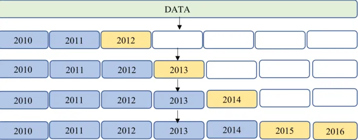
In this project, observations dependent on time. Therefore, it is not possible to keep a model blind about this dependency. Due to this kind of data in this project, random separation does not work. The data should be cut off based on time. For example, older dates are determined as training set and recent dates are considered as test set.

A common approach is used to produce a better estimation of error forecast of a model, which is called forward chaining and referred as rolling-origin. In this technique, the full data is split into k-fold train/test subsets (Bergmeir & Benitez, 2011). Each time, a specific year is considered as a test data and the previous year or years are taken as a training set. This process keeps moving forward through the data, until it covers all the dataset. The trained models with each test data produce new predicted values. Therefore, the difference between predicted and actual values is computed by the considered metric performance in this study. Afterwards, the final error is obtained by taking the average of k folds results.

3.5 Data Modeling

The main goal of this study is to compare sets of supervised machine learning algorithms, such as multiple regression, regression tree, random forests, gradient boosting, and LSTM and GRUs recurrent neural networks. They are reputed as the most accurate forecasting models. Therefore, these algorithms will be implemented to create the models. As discussed before, the target of this project is applying the mentioned supervised learning techniques to forecast the amount of consumed hours and mileage, individually, in Communauto carsharing operator in time scale.

3.5.1 Multiple Regression

One of the extensions of simple linear regression is called multiple regression. In particular, it is an effective tool for forecasting problems with estimating the relationships between independent variables or features and quantitative dependent values or output. Multiple regression does not assume a linear relationship between response and features.

General format of this model is as follows:

𝑌 = 𝛽_c+ 𝛽&𝑋& + 𝛽/𝑋/+ ⋯ + 𝛽3𝑋3 + 𝜀 (3.7) Where if there are p features in dataset, 𝑋₃ refers to the pth feature, Y is the response value and 𝜀 is a random error term. 𝛽 is regression coefficient which is unknown. This method is traced to find the best estimation that the model fits the available data well and minimizes the error rate. It is often more convenient to use matrix notation:

𝑌 = 𝑋𝛽+ 𝜀 (3.8) 𝑌 is 𝑛 × 1 vector: 𝑌 = h𝑦⋮& 𝑦_'j X is 𝑛 × (𝑝 + 1) matrix: X = m1⋮ 1 𝑥&& ⋯ 𝑥&n ⋮ ⋱ ⋮ 𝑥_p& ⋯ 𝑥_pnq 𝛽 is (𝑝 + 1) × 1 vector: 𝛽 = r 𝛽_c ⋮ 𝛽_ns 𝜀 is 𝑛 × 1 vector: 𝜀 = h𝜀⋮& 𝜀_'j

The estimated unknown coefficient is achieved by minimizing the sum of square errors method. This is implemented by taking the first derivative of sum of the squared errors with respect to estimated coefficient or βu . Then, set the derivative is set to equal zero (Lang, 2013).

The sum of the squared errors:

v 𝑒̂₊/ _{= v(𝑦} + − 𝑦-+)/ ' +0& ' +0& = (𝑦 − 𝑋𝛽y)z (𝑦 − 𝑋𝛽y)

= 𝑦z𝑦 − 𝑋𝛽y − 𝛽yz𝑋z𝑦 + 𝛽yz𝑋z𝛽y Take derivative with respect to 𝛽y:

{(\|\Q }~•Q ~•_{~•€}€•‚ ~•€}€ƒ~• ) = 0

−2X…𝑦 + 2X…X𝛽y = 0

X…𝑦 = X…X𝛽y 𝑦 Therefore:

𝛽y = (X…_X)Q&_𝑋z_{𝑦 (3.9)}

Regression coefficient refers to the change in Y associated with a one-unit change in the respective independent variable. Statistical tests try to find whether each coefficient is significantly different from zero.

Furthermore, linear correlation coefficient is used to determine the dependency of variables, which is in range of +1 or −1. When the value is close to zero, it means there is no linear relationship. If correlation goes to near minus or plus one, it indicates a strong linear relationship between those variables. Multiple regression examines the subset or full features to come up to the combination of them, which leads to the best result. In some situations, regression analysis cannot detect a relationship, because of circle form. For this reason, creating plot is as an alternative way to

mapping a causal effect relationship between features and dependent variables. Therefore, in some circumstances, more complex model may contain variables with higher powers. For instance:

𝑌 = 𝛽c+ 𝛽&𝑋 + 𝛽/𝑋++ ⋯ + 𝜀G i = 2,… (3.10) Sometimes, two or more variables have a significant relationship. Therefore, the effect of their interaction is considered in procedure of creating model. For example:

𝑌 = 𝛽_c+ 𝛽&𝑋& + 𝛽/𝑋/+ 𝛽&/(𝑋&𝑋/) + ⋯ + 𝜀G (3.11) Therefore, the combination of these terms creates multiple regression. The associated p-value and individual t-statistics is applied to test whether a variable contributes significantly to the fitted model. The level of significant p-value is considered 0.05 for inclusion of a variable in the structure of a model and rejection the null hypotheses (𝐻_c ):

𝐻_c : 𝛽_G = 0

The results of regression are easily interpretable, and the pattern can be recognized by plots (James et al., 2013). But, this model is sensitive to outliers, and such points can seriously affect the final results.

3.5.2 Regression Tree

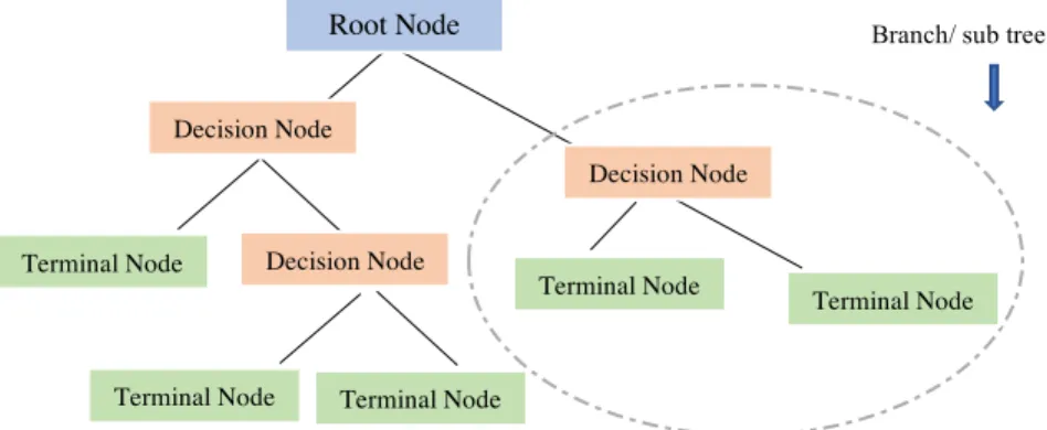
Regression tree is first proposed by Breiman and colleagues in 1980 (Breiman, 2001). Regression tree is an alternative approach of nonlinear regression, and it is most widely used in regression problems. It means that this model can be constructed as a forecasting model in dataset, where dependent variables or output lying in a numeric range. The implementation of forecasting action is set by partitioning the data into smaller regions. The obtained segmentations are more manageable and can be summarized in a tree with terminal nodes or leaves and branches. Then, the operation of partitioning splits the subdivisions again, which is called recursive partitioning. This tree allows variables to be a mixture of categorical, continuous, sparse, skew, etc. Even this model is compatible with missing values in the dataset. Structure of the tree is able to adapt to large data with no requirement to know the correlation between each individual feature variable and response (Strobl, Malley, & Tutz, 2009).

Figure 3.2 shows a top-down tree, which is started from root node with querying a sequence of questions about features and places a feature as a representative at this node. Decision node refers

to sub-node, when it is divided to further sub-nodes. In contrast, when a node does not divide, it is called leaf or terminal node. The nodes are accumulated with questions, and branches between nodes are labeled by the answers. Next question depends on answers to overhead questions. Finally, each part of the observations is assigned to subset with similar response values, and the rest are assigned in other subgroups. So, the goal of all the efforts is to achieve an optimal partitioning of the data.

Figure 3-2: A recursive partitioning tree

There are different splitting criteria in regression tree, in-which MSE (mean squared error) as one of them is popular. Firstly, in order to perform division, one feature as root node which leads to the lowest MSE, is selected. In each node, 𝑦-+, as the response mean of the training sample, and MSE are calculated separately within node (depicted in (3.12)). For example, observation 𝑋 = 𝑥 when 𝑥 𝜖 𝑁_G, 𝑦-₊ is the predicted value, 𝑁_G refers to 𝑗𝑡ℎ node.

𝑦-+ = &_‹ ∑‹+0&𝑦+ (3.12) Thereafter, the value with significant MSE will be chosen to best split the tree at that particular step. The process will elaborate for other observations in training set.

Ideally, the goal of this method is finding a partition with lowest mean squared error for given regression problem. Recursive splits on dataset continue upon reaching the state of defined

Root Node

Decision Node

Terminal Node Decision Node

Branch/ sub tree

Terminal Node Terminal Node

Decision Node

Terminal Node Terminal Node