Neutrino propagation in dense astrophysical environnements : beyond the standard frameworks

(1)

HAL Id: tel-02466847

https://tel.archives-ouvertes.fr/tel-02466847

Submitted on 4 Feb 2020

HAL is a multi-disciplinary open access

archive for the deposit and dissemination of sci-entific research documents, whether they are pub-lished or not. The documents may come from teaching and research institutions in France or abroad, or from public or private research centers.

L’archive ouverte pluridisciplinaire HAL, est destinée au dépôt et à la diffusion de documents scientifiques de niveau recherche, publiés ou non, émanant des établissements d’enseignement et de recherche français ou étrangers, des laboratoires publics ou privés.

Neutrino propagation in dense astrophysical

environnements : beyond the standard frameworks

Amelie Chatelain

To cite this version:

Amelie Chatelain. Neutrino propagation in dense astrophysical environnements : beyond the stan-dard frameworks. Physics [physics]. Université Sorbonne Paris Cité, 2018. English. �NNT : 2018US-PCC224�. �tel-02466847�

(2)

Thèse de doctorat de l’Université Sorbonne Paris Cité

Préparée à l’Université Paris Diderot

École doctorale des Sciences de la Terre et de l’Environnement et Physique de l’Univers,

Paris - ED 560

Laboratoire AstroParticules et Cosmologie (APC) - Groupe théorie

Neutrino propagation in dense astrophysical

environments: beyond the standard frameworks

Thèse de Doctorat - Spécialité : Physique Théorique

présentée par

Amélie Chatelain

dirigée par

Maria Cristina Volpe

et soutenue publiquement le 13 décembre 2018 à Paris devant un jury composé de :

Présidente du jury Danièle Steer Professeure Université Paris Diderot

Rapporteur Carlo Giunti Professeur Università di Torino et INFN

Rapporteure Gail McLaughlin Professeure North Carolina State University

Examinatrice Sacha Davidson DR-CNRS Université de Montpellier

(3)

(4)

Thesis advisor: Professor Maria Cristina Volpe Amélie Chatelain

Neutrino Propagation in dense astrophysical environments: beyond the

standard frameworks

Abstract

Since the discovery of neutrino oscillations in vacuum, it has been shown that the presence of a matter background can greatly modify the flavor evolution. The inclusion of neutrino self-interactions in the stud-ies of neutrino flavor conversions in dense astrophysical environments has triggered an intense theoretical ac-tivity. This thesis enters into this context by going beyond usual approaches. In our first project, we explore analytically and numerically the so-called helicity coherence, using for the first time a detailed astrophysical simulation of binary neutron star merger remnants. This study shows that helicity coherence cannot lead to conversions and, by doing so, strengthens the validity of the usually-employed mean-field equations in dense media. It also brought a better understanding of the nonlinear feedback mechanism. Having done so, we examine in a second part the role of nonstandard matter-neutrino interactions in the same astrophys-ical setting. We find that the presence of such interactions creates another MSW-like resonance, called the inner resonance, which can have an interesting interplay with the matter-neutrino resonance, and leads to flavor conversions very close to the central object. We also analyze the mechanism of such a resonance and show that it can be met as a synchronized resonance in the presence of a strong self-interaction potential. Finally, our last study is more formal, as it focuses on the fundamental question of decoherence by wave-packet separation in the presence of strong gravitational fields. We use the density matrix formalism for the neutrino wave packet in the Schwarzschild metric and derive the expression of the coherence length. This work provides with the first study in the description of decoherence in curved space-time.

Keywords: neutrinos, astrophysics, binary neutron stars, helicity coherence, nonstandard, wave packets.

Depuis la découverte des oscillations de neutrinos dans le vide, il a été démontré que la présence d’un environnement de matière peut avoir une grande influence sur les changements de saveurs. L’inclusion des termes d’interactions neutrino-neutrino dans les études des conversions de saveurs dans les environnements astrophysiques denses a créé une activité théorique très intense. Cette thèse entre dans ce cadre en allant au-delà des approches usuelles. Dans notre premier projet, nous explorons analytiquement et numériquement le rôle de la cohérence d’hélicité, en nous basant pour la première fois sur une simulation astrophysique dé-taillée d’un rémanent de fusion de système binaire d’étoiles à neutrons. Cette étude montre que la cohérence

(5)

Thesis advisor: Professor Maria Cristina Volpe Amélie Chatelain habituellement utilisées dans les milieux denses. Elle apporte également une meilleure compréhension du mécanisme de nonlinear feedback. Après cela, nous examinons dans une seconde partie le rôle des interac-tions non-standards entre matière et neutrinos dans le même contexte astrophysique. Nous trouvons que la présence de telles interactions peut créer une nouvelle résonance de type MSW, appelée la résonance ”in-ner”, qui peut avoir un couplage intéressant avec la résonance matière-neutrino, et provoque des conversions de saveurs très proches de l’objet central. Nous analysons également le mécanisme d’une telle résonance, et montrons qu’elle se manifeste comme une résonance synchronisée en présence d’un potentiel d’interaction neutrino-neutrino fort. Enfin, notre dernière étude est plus formelle et se focalise sur la question fonda-mentale de la décohérence par séparation de paquets d’ondes en présence de champs gravitationnels forts. Nous utilisons le formalisme de la matrice densité pour le paquet d’onde du neutrino dans la métrique de Schwarzschild, et dérivons l’expression de la longueur de cohérence. Ce travail constitue la toute première étude dans la description de la décohérence en espace-temps courbe.

Mots clés : neutrinos, astrophysique, systèmes binaires d’étoiles à neutrons, cohérence d’hélicité, non-standard, paquets d’ondes.

(6)

Acknowledgments

I would like to thank all the people who accompanied me during this journey.

My first thought goes to Cristina, who accepted me as a Ph.D. student despite not looking for one. She introduced me and guided me to the fascinating field of neutrino physics and was always there to help. I am infinitely grateful for her help and moral support in particular during the past few months, without which this would not have been possible. I feel privileged to have had the opportunity to work with her over the past three years.

I also would like to thank Gail Mclaughlin and Carlo Giunti for agreeing to be my referees, and my jury members Sacha Davidson and Daniele Steer, some of whom traveled for attending my defense.

Working in the theory group at APC was a pleasure for me, and I would like to thank all its staff and mem-bers for welcoming me there. I value the fun times I spent with the Ph.D. students I got to know during my stay, in particular, Cyrille, Félix, Frédéric, Gabriel, Jan, Leandro, Makarim, Maxime, Pierre and Theodoros. I also would like to express my appreciation to my friends Damien, Mathilde and Yasin for making my life easier and more enjoyable during the course of this thesis.

Finally, I would like to express my gratitude to my family whose support has been invaluable to me. There are not enough words to thank you enough.

(7)

1

General introduction

The existence of neutrinos was first proposed in 1930 by Wolfgang Pauli, in order to explain the continuous spectra of beta particles emitted in beta decay. The word ”neutrino” itself was introduced to the scientific community by Enrico Fermi in two conferences —Paris, in July 1932 and the Solvay conference in October 1933—, to differentiate this new, neutral particle from the heavier neutron. In 1934, Fermi postulated his theory on beta decay, in which four fermions, including the neutrino, were interacting with one another. This work was first submitted to Nature which rejected it, judging it ”too remote from reality to be of in-terest to the reader”. Today, we know that Fermi’s theory corresponds to the low-energy limit of the weak interaction.

However, it was only in 1956 that neutrinos were detected for the first time. Cowan, Reines, Harrison, Kruse and McGuire [1] announced the first detection of reactor electron antineutrinos through inverse beta decay. The produced neutrons are captured on nuclei while the produced positrons annihilate with electrons, both processes emitting photons that could be detected. Later, the first muon neutrino was detected in 1962 by Lederman, Schwartz, and Steinberger, hence showing that more than one type of neutrino exists. The third lepton flavor, tau, was discovered in 1975 at the Standford Linear Acceleration Center and assumed to have an associated neutrino. However, it was directly measured only in 2000 by the DONUT collaboration at Fermilab.

In the late 60s, the Homestake experiment, headed by Davis detected and counted neutrinos emitted by nuclear reactions in the Sun [2]. They observed a discrepancy in the number of neutrinos detected, with the

(11)

problem. This problem remained unsolved for about thirty years, triggering numerous experiments and lead to the discovery of neutrino oscillations in 1998 [3]. In 1957, Pontecorvo introduced first the idea of neutrino-antineutrino conversions by analogy with kaon oscillations [4]. After the existence of muon neutrinos was established, Maki, Nakagawa and Sakata introduced in 1962 the notion of flavor mixing [5], leading to νe ↔

νµand ¯νe↔ ¯νµoscillations. Pontecorvo further elaborated on those oscillations in 1967. After the discovery

of the solar neutrino problem, Gribov and Pontecorvo published the first modern treatment of neutrino oscillations, introducing neutrino masses in an article called ”Neutrino astronomy and lepton charge” [6]. The Homestake measurement of solar neutrinos and the first detection of supernova neutrinos in 1987 were two milestones for the field of neutrino astronomy.

The discovery of neutrino oscillations by the SuperKamiokande (1998) [3] and SNO (2001) [7] experi-ments has proven that neutrinos are elementary massive particles with mixing, that is the mass (or propaga-tion) basis and the flavor (or interacpropaga-tion) basis do not coincide. Since then, precision measurements have determined most of the fundamental neutrino oscillation parameters. Crucial open questions remain, in particular, the nature of neutrinos (Majorana or Dirac), the neutrino mass ordering, the existence of sterile neutrinos and of CP violation in the lepton sector. It is also still unknown how neutrino masses are gener-ated.

As neutrinos are very light and interact only through weak interactions, they also make wonderful mes-sengers of the universe. Expanding the work of Wolfenstein [8], Mikheev and Smirnov noted in 1985 [9] that neutrino oscillations could be drastically modified in the presence of a matter background. In particu-lar, they showed the existence of the so-called Mikheev-Smirnov-Wolfenstein (MSW) resonance that could be met in the Sun. It is now well-established that the MSW phenomenon is at the origin of the high-energy

8_{B solar neutrinos deficit.}

Flavor evolution in dense astrophysical environments, such as core-collapse supernovae or compact bi-nary objects, has turned out to be a complex problem. Indeed, the presence of neutrino self-interactions in such environments makes the study of neutrino evolution a nonlinear problem [10]. The inclusion of self-interaction terms [11] has triggered more than a decade of intense theoretical investigations, and models of increasing complexity are used to unravel new flavor instabilities and mechanisms such as collective con-version phenomena. Such studies are necessary to assess the actual impact of neutrino oscillations on the physics of the environment, in particular, on the dynamics of supernovae, on the nucleosynthetic r process abundances as well as for future observations of supernova neutrinos and of the diffuse supernova neutrino background. Understanding the mechanism for the explosion of massive stars and identifying the sites where heavy elements are produced (r process) are two key longstanding open questions in astrophysics.

(12)

The recent observation of gravitational waves from a binary neutron star merger event GW170817 [12] coincidently with a short gamma-ray burst and a kilonova constitute the first direct evidence for r process nucleosynthesis in such sites. Moreover, recent works have shown that a significant part of the r process elements is likely to be produced in the so-called neutrino-driven winds. Therefore, fully understanding neutrino flavor conversions in this type of environment, as well as their role in nucleosynthesis is primordial.

The main goal of the present thesis is to investigate neutrino flavor conversions in dense astrophysical en-vironments beyond the standard frameworks. We do so in three respects, encompassing the exploration of the role of helicity coherence which is usually neglected, the effects of nonstandard interactions and neutrino decoherence by wave packet separation.

The first project of this thesis is a study of the so-called helicity coherence correlators, which appear as nonrelativistic corrections to our neutrino evolution equations. The corresponding contributions, propor-tional to the absolute mass of neutrinos, create a coupling between active and sterile neutrino components (”wrong helicity” components) in case of Dirac neutrinos, or between neutrinos and antineutrinos in case of Majorana neutrinos. While one first study of these terms has been done in a very simple model with one Majorana neutrino flavor [13], no study was ever made on the effect of this new coupling in a realistic sce-nario. In the first toy model, the authors found that the presence of helicity coherence coupling could create a MSW-like resonance between neutrinos and antineutrinos, which could be amplified by a nonlinear feed-back, created by the nonlinear nature of the equations, inducing strong flavor conversions. Our goal in this thesis is to investigate the possible effects of helicity coherence coupling neutrinos to antineutrinos in a real-istic framework with two Majorana neutrino flavors, based on detailed astrophysical simulations of a binary neutron star merger remnants. After re-deriving the most general equations for neutrino propagation in the mean-field approximation, we numerically explore a large number of trajectories as well as a large parame-ter range. We find that MSW-like resonance conditions between neutrinos and antineutrinos can be met in this detailed astrophysical scenario. We also analyze analytically our results in the light of nonlinear feed-back, discussing general conditions for multiple MSW-like resonances that would increase the adiabaticity. Our results also shed light more generally on nonlinear feedback mechanisms, which are observed in binary neutron star mergers simulations such as the one associated with a flavor phenomenon called the matter-neutrino resonance. The work presented in this thesis constitutes the first realistic investigation considering helicity coherence and allows to assess the validity of the usual mean-field equations used in flavor evolution studies.

(13)

interac-nonstandard interactions, obtained with scattering and oscillation experiments, are still rather loose. The presence of NSI would modify the interpretation of oscillation experiments and may explain observed anoma-lies. Studies of these interactions in core-collapse supernovae [14,15,16,16] have shown that they can alter neutrino flavor conversions, in particular by creating a new MSW resonance called the Inner (I) resonance extremely close to the neutrino emission surface. Because of its location, this new resonance could have a strong effect on r process nucleosynthesis. We explore for the first time the role of NSI in binary neutron star merger remnants through numerical simulations and show that the I resonance condition can also be met, creating strong flavor conversions very close to the neutrino emission surface. Moreover, we shed a new light on its mechanism and show that it can be interpreted as a synchronized MSW resonance in the presence of a significant self-interaction potential. This aspect of the I resonance has been overlooked in previous stud-ies of NSI in core-collapse supernovae. Flavor conversions due to NSI such as the I resonance can have a strong impact on the electron fraction —the proton-to-baryon ratio, which is a key parameter for r process nucleosynthesis— as they are occurring very close to the central object, and could modify the abundances of the elements produced through r process in the neutrino-driven winds. We discuss the potential impact of NSI on the electron fraction in this environment.

The third project of the thesis goes towards a more fundamental direction with respect to the previous two. In fact, it focuses on the investigation of decoherence by wave-packet separation on neutrino flavor conversions, and in particular the effects of curved space-time. Indeed, as neutrinos are described by wave packets rather than plane waves, it is possible for them to separate, leading to a damping of the oscillation terms. After discussing the wave-packet description in dense astrophysical environments, we rederive consis-tently the coherence length in flat space-time using the density matrix formalism and discuss the inclusion of adiabatic matter effects. Then, we investigate the differences arising when considering the propagation of neutrinos in strong gravitational fields. This is still an ongoing project for which final results have not been included yet because of lack of time.

The thesis is organized as follows. First, we present the current understanding of neutrino physics in Chap-ter 2. We discuss both the theoretical aspects of neutrino propagation in dense astrophysical environments and the current status in neutrino physics. In Chapter 3, we describe the astrophysical scenarios of core-collapse supernovae and binary neutron star merger remnants, as well as the neutrino emissions and key features of their propagation in these environments. The following chapters are dedicated to the original work developed in the course of this thesis, studying neutrino propagation in dense astrophysical environ-ments beyond the standard frameworks. The role of helicity coherence correlators and nonlinear feedback mechanisms are explored in Chapter 4 in the context of binary neutron star merger remnants. In Chapter 5,

(14)

we present a study of the effects of nonstandard interactions on neutrino propagation in the same astrophys-ical setting. The numerastrophys-ical results presented in Chapters 4 and 5 have been obtained using a FORTRAN (90/95) developed during the course of this thesis. Decoherence by wave-packet separation in vacuum and in the presence of gravitational fields is discussed in Chapter 6. In order to maintain the readability of this manuscript, some calculations are detailed in the Appendices while only their main results are discussed in the text. Our Conclusions are presented at the end of the manuscript.

The results obtained have made the object of two publications

• [17] A. Chatelain and M.C. Volpe, Helicity coherence in binary neutrino star mergers and nonlinear

feedback, Phys.Rev.D95 (2017) no.4, 043005.

• [18] A. Chatelain and M.C. Volpe, Neutrino propagation in binary neutron star mergers in the presence

(15)

Unless specified otherwise, we adopt the following conventions and notations • Natural units are usedℏ = c = kB = G = 1,

• The signature of the metric is chosen to be (−, +, +, +), • Greek indices µ, ν, ... run from 0 to 3.

• ηµν = ηµν =diag (−1, +1, +1, +1) is the Minkowskian metric,

• γµ_{denotes one the usual gamma matrices, satisfying the Clifford algebra}_{γµ_{, γ}ν_{} = 2η}µν_{and γ}

5is

defined as γ5 ≡ iγ0γ1γ2γ3,

• Feynman slash notation is used: /a = aµγµ,

(16)

2

Theory of neutrino oscillations

model, in which neutrinos get a mass, and introduce the notion of mixing. We discuss the differences be-tween Majorana and Dirac neutrinos and show a first derivation of neutrino oscillation probabilities in vac-uum. In Section 2.2, we derive the most general evolution equations for the neutrino density matrix in media in the mean-field approximation and the element of the Hamiltonian involved in those equations. We dis-cuss the limit of a homogeneous system and ultra-relativistic neutrinos. In Section 2.3, we use the equations derived above to study the propagation of neutrinos in matter and show that the coupling to matter gives rise to a resonance phenomenon called the Mikheev-Smirnov-Wolfenstein effect. Finally, in Section 2.4, we present a brief overview of the experimental status of the domain.

2.1 Introduction to neutrino physics 2.1.1 Neutrinos in the standard model

In the standard model (SM) of particle physics, neutrinos are introduced as massless particles sub-ject only to the weak interaction. Neutrinos are fermions (intrinsic spin 1/2 particles), which exist in three leptonic flavors: the electron neutrino, the muon neutrino, and the tau neutrino1.

The fermionic free Lagrangian density is given by [20]

L0(x)≡ − ¯ψ (x)

(

/

∂ + m)ψ (x) , (2.1)

where m is the mass of the fermion, created through a Yukawa-type coupling between the fermionic field and the Higgs boson. The fermionic field ψ can be expressed

ψ (x) = ∫ d3_⃗_q (2π)3/2 ∑ σ=±1/2 (

u(⃗q, σ)eiqxa(⃗q, σ) + v(⃗q, σ)e−iqxb†(⃗q, σ)), (2.2) where σ is the spin, p the four-momentum vector, u and v are four-component Dirac spinors, and a and b are, respectively, the standard particle and antiparticle annihilation operators. The equal-time anti-commutation relations are

{a(⃗q, σ), a†_(⃗_q′_{, σ}′₎_{} = {b(⃗q, σ), b}†_(⃗_q′_{, σ}′₎_{} = δ}

σ,σ′δ(3)(⃗q− ⃗q′), (2.3)

{a(⃗q, σ), a(⃗q′_{, σ}′₎_{} = {b(⃗q, σ), b(⃗q}′_{, σ}′₎_{} = 0.} _(2.4)

To describe massless fermions, we introduce the projectors PL = 1−γ₂ 5 and PR = 1+γ₂ 5. In the SM of

particle physics, neutrinos are supposed to be massless fermions interacting only through their left-handed

(18)

component ψL = PLψ through Charged Current (CC) and Neutral Current (NC) interactions, with the

Lagrangian densities respectively given by

LCC = ig 2√2 ∑ α=e,µ,τ ¯ ψναγ µ₍₁_{− γ} 5)ψαWµ+ h.c.≡ ig 2√2j µ WWµ+ h.c., (2.5) LN C = ig 2 cos θW ∑ α=e,µ,τ (_¯ ψναγ µ (cνα v − c να a γ5)ψνα+ ¯ψαγ µ (cα_v − cα_aγ5)ψα ) Zµ ≡ ig 2 cos θW j_ZµZµ, (2.6) where g ≡ _{sin θ}e

W is the electro-weak coupling constant, e being the electric charge and θW the Weinberg

angle, ψxdenotes the fermionic field of the particle x, and cxv, cxaare the vector and axial coupling constants

of the particle x, related to its isospin and its charge. W and Z are two bosonic vector fields, respectively the charged and neutral weak interaction gauge boson fields, of masses mW and mZ.

It is interesting to notice that the masses of the vector bosons W and Z are of the order of 100 GeV, which is much larger than the energy involved in the phenomena considered here. Therefore, the propagators of the massive bosons Z and W can be simplified (for example, for W )

−i (2π)4 ηµν+ p_mµ2pν W p2_{+ m}2 W |p|2_≪m2 W −→ −i (2π)4 ηµν m2 W , (2.7)

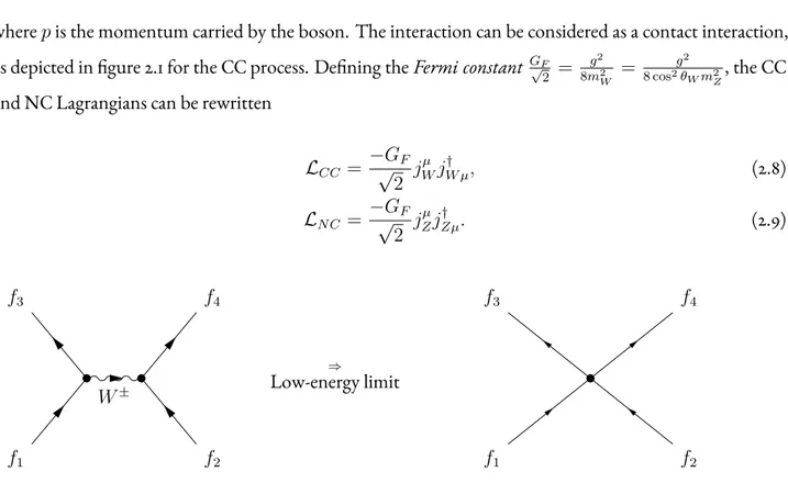
where p is the momentum carried by the boson. The interaction can be considered as a contact interaction, as depicted in figure 2.1 for the CC process. Defining the Fermi constant G_√F

2 = g2 8m2 W = _{8 cos}2g_θ2 Wm2Z, the CC

and NC Lagrangians can be rewritten

LCC = −G F √ 2 j µ WjW µ† , (2.8) LN C = −G F √ 2 j µ ZjZµ† . (2.9) W± f1 f2 f3 f4 ⇒ Low-energy limit f1 f2 f3 f4

Figure 2.1:In the low-energy limit, the CC (or NC) interaction involving the propagation of a vector bosonW(orZ) becomes a contact interaction.

(19)

masslessness of neutrinos. Yet, the discovery and experimental confirmation of neutrino oscillations [3] imply the existence of massive neutrinos and mixings. Thus, to have a more complete understanding of neutrinos, it is necessary to extend the SM. In the next section, we will introduce the minimally extended

Standard Model, in which right-handed neutrinos exist.

2.1.2 Massive neutrinos and mixing Dirac neutrinos

Neutrinos are neutral leptons, and since their charged-leptonic partners e, µ, τ are Dirac fermions, it is nat-ural to consider them as such. In the minimal extension of the SM, Dirac fermions, namely leptons and quarks, acquire their mass through the Higgs mechanism. The Dirac mass term reads, for a fermion of mass

mD

LD

mass=−mDψψ =¯ −mDψ¯RψL+ h.c.. (2.10)

However, the mass term and the CC interaction term are not necessarily diagonal in the same basis: neutrinos with a definite mass are not necessarily neutrinos with a definite flavor. This phenomenon is known as

neutrino mixing and is responsible for neutrino oscillations.

From now on, we will denote by νka neutrino with a definite mass mk, and ναa neutrino with a definite

flavor α: the basis|νk⟩ is called the mass basis, while |να⟩ is called the ﬂavor basis. These two bases are related

by a 3× 3 unitary matrix U, called the Pontecorvo - Maki - Nakagawa - Sakata (PMNS) matrix

|να⟩ =

∑

k

U_αk∗ |νk⟩ . (2.11)

Rewriting the weak leptonic current in the mass basis j_Wµ = ∑_α=e,µ,τ∑_k=13 U_αk∗ ψ¯νkγ

µ₍₁_{− γ}

5)ψα, it

be-comes obvious that flavor eigenstates, created through weak interactions, are a mixture of massive eigenstates. A n× n unitary matrix has n2_{real independent parameters which can be parametrized by}n(n−1)

2 angles and

n(n+1)

2 phases. However, because of the invariance of the Lagrangian under global phase transformations,

2n− 1 phases can be eliminated. Therefore, in the case of three Dirac neutrinos, the PMNS matrix depends on three mixing angles, θ12, θ23, θ13and one CP-violating phase, δ, and can be parametrized as

U =      1 0 0 0 c23 s23 0 −s23 c23           c13 0 s13e−iδ 0 1 0 −s13eiδ 0 c13           c12 s12 0 −s12 c12 0 0 0 1     , (2.12)

(20)

Majorana neutrinos

In 1937, Majorana suggested that the left-handed and right-handed component of the neutrino field, ψLand

ψR, are not independent [21]. Let us define the charge-conjugate of a field ψ, ψc =C ¯ψ⊺, whereC = iγ2γ0

is the charge-conjugation matrix and⊺ the transpose [19]. Then, one may notice that ψ c

L is right-handed,

namely PLψLc = 0. It is also possible to check that ψLctransforms as ψLunder a Lorentz transformation.

As a consequence ψLand ψLccan, in principle, form a mass term, called the Majorana mass term

LL mass=− 1 2m ¯ψ c LψL+ h.c., (2.13)

where the factor 1/2 comes from the fact that ψLand ψLcare not independent.

A Majorana field is therefore a field that satisfies the Majorana condition ψR = ψLc, which can also be

re-expressed ψ = ηψc_{(where η is a phase) by defining ψ = ψ}

L+ ηψLc. This condition requires the Majorana

field to be neutral, and neutrinos are (currently) the only known neutral fermions.

In terms of annihilation and creation operators, a Majorana fermionic field has a similar expression to the Dirac field (2.2), but with the additional relation b(⃗q, σ) = a(⃗q, σ), namely

ψ_νM i (x) = ∫ d3_⃗_q (2π)3/2 ∑ σ=±1/2 (

ui(⃗q, σ)eiqxai(⃗q, σ) + vi(⃗q, σ)e−iqxa†i(⃗q, σ)

)

. (2.14)

By convention, left-handed neutrinos are called neutrinos while right-handed neutrinos are called anti-neutrinos. It is worthwhile to note that a Majorana neutrino has half as many degrees of freedom as a Dirac neutrino (see figure 2.2). Indeed, from CPT invariance and Lorentz invariance, there are four possible helicity states for a Dirac neutrino of a given momentum: νL, νR, ¯νLand ¯νR. However, as a Majorana field is self-charge

conjugated, a CPT transformation only modifies its helicity, hence there are only two possible states for a Majorana neutrino of a given momentum νLand νR.

The presence of neutrino mixing doesn’t depend on the nature of neutrinos. There exists a mixing matrix

U such that|να⟩ =

∑

kUαk∗ |νk⟩. However, there is a major difference between Dirac and Majorana

neu-trinos. In the case of massive Dirac neutrinos, 2n− 1 phases of the mixing matrix are eliminated because of the invariance of the Lagrangian under global phase transformations, but for Majorana neutrinos, the mass term is not invariant: if ψνk,L → ψ

′ νk,L = e iϕk_ψ νk,L, then ¯ψ c νk,L → ψ ′ νk,L = e iϕk_ψ¯c

νk,L and the lepton

number is violated. As a consequence, only n phases, corresponding to the re-phasing of the charged lepton fields, can be eliminated. Therefore, in the case of three flavors, if neutrinos are Majorana particles, there are two additional phases in the PMNS mixing matrix.

(21)

νL ν¯R ν¯L νR Lorentz Boosts CPT CPT Lorentz Boosts νL νR Lorentz Boosts CPT Lorentz Boosts

Figure 2.2:Dirac (left) and Majorana (right) degrees of freedom.

tons, that is a double beta decay process with the emission of two electrons. This lepton-number-violating phenomenon can occur only if a right-handed antineutrino emitted at a vertex can be reabsorbed at another vertex as a left-handed neutrino, which would imply neutrinos are Majorana particles. This process is yet to be detected.

It is, therefore, possible to describe massive neutrinos with a single chiral component. Another Majorana mass term can be introduced in extended versions of the SM asLR

mass = −12m ¯ψ

c

RψR+ h.c., where ψR

describes a sterile, right-handed neutrino field. The so-called seesaw mechanism relies on the existence of this mass term. This mechanism, proposed in the seventies, explains the lightness of the left-handed active neutrinos with the presence of very heavy, sterile, right-handed neutrinos. It assumes that neutrino masses are described by the Dirac and Majorana mass term, which is the most general mass term for Majorana neu-trinos, involving both left-handed and right-handed neutrinos. In the following, we describe the main idea of this mechanism.

We consider here the simplest case in which only one generation of neutrino exists, with two neutrino fields νLand νR. The Dirac and Majorana mass term can be written in the matrix form

LD+M mass =− 1 2n¯LM n c L + h.c., (2.15) where nLis a vector nL=  νL ν c R   , (2.16)

and M is the mass matrix

M =  mL mD mD mR   . (2.17)

(22)

a unitary matrix U so that (see e.g. Ref. [22]) U⊺M U =  m1 0 0 m2   , (2.18)

with the eigenvalues m1, m2given by

m1 = 1 2 mR+ mL− √ (mR− mL) 2 + 4m2 D , (2.19) m2 = 1 2 mR+ mL+ √ (mR− mL) 2 + 4m2 D . (2.20)

The mass term (2.15) can then be rewritten

LD+M mass =− 1 2 ∑ i=1,2 miν¯iνj, (2.21)

where the fields ν1and ν2describe Majorana particles of definite masses

 ν1 ν2   = U†_n L+ ( U†nL )c . (2.22)

The matrix U can be parametrized [19] as

U =   cos θ sin θ − sin θ cos θ    eiλ 0 0 1   , (2.23)

with θ ∈[0,π₂]and λ∈ [0, 2π]. Using Eq. (2.18), we find for those parameters the relations tan 2θ = 2mD

mR− mL

, (2.24)

and tan 2λ = 0, as we assumed mL, mR, mDare real parameters.

The main assumptions of the seesaw mechanism presented here are the following

1. Assume that the Majorana mass term is null, that is mL = 0. This is a natural assumption, as the

presence of such a term is forbidden by the symmetries and renormalizability of the SM (see Ref. [19]).

2. Assume that the Dirac mass mDis generated through a standard Higgs mechanism, and is therefore

(23)

mR ≫ mD.

With these assumptions, the eigenvalues (2.19-2.20) become

m1 ∼ m2 D mR ≪ m D, (2.25) and m2 ∼ mR ≫ mD. (2.26)

Therefore, m1is very light compared to other leptons, while m2is very heavy. The parameter θ (2.24)

be-comes very small: ν1 is mostly composed of active νLwhile ν2 is mostly composed of sterile νR. This is

the so-called seesaw mechanism: a very heavy right-handed neutrino is responsible for the lightness of the left-handed neutrino.

The suppression factor, mD

mR, depends on the scale on which the lepton number is violated. Note that if

we take mD ≈ 102GeV, and if we consider mRto be of the order of the grand-unification scale mD ≈

1014_{− 10}16_{GeV, then we find}mD

mR ≈ 10

−14_{− 10}−12_{: the seesaw mechanism would explain why neutrino}

masses are so small compared to other leptons.

As described above, the inclusion of neutrino mass terms and mixing make it possible for neutrinos to change their flavors, leading to the phenomenon of neutrino oscillations. In the section below, we discuss the simplest case of neutrino oscillations in vacuum.

2.1.3 Neutrino oscillations in vacuum

Neutrinos are produced through CC interaction processes and are therefore produced as flavor eigenstates which are superpositions of mass eigenstates. Because the mass eigenstates have non-zero and non-degenerate masses, and because of mixing, the superposition detected after propagation is not necessarily the same as the initially produced one: the neutrino detected may have changed its flavor. This phenomenon, first in-troduced by Bruno Pontecorvo in 1957 [4, 23], has been discovered by the SuperKamiokande and SNO experiments [3,24]. In this section, we will present the standard derivation of the neutrino oscillation prob-abilities.

Let us assume that a neutrino of flavor α and momentum ⃗q is created through a CC weak process at the instant t = 0. As we have seen before, it is created as a pure flavor state and can be written as

|να⟩ =

∑

k

(24)

Note that the number of massive neutrinos is not limited: its minimum is three, but it may be larger than three. If so, the additional neutrinos in the flavor basis would be sterile, namely, they would not participate in any interaction except gravity. Therefore, the number of massive neutrinos will not be specified in the following general derivation. We consider orthonormal massive neutrino states:⟨νl|νk⟩ = δkl, and since U

is unitary,⟨να|νβ⟩ = δαβ.

In a Schrödinger-like picture, the massive neutrino states are eigenvalues of the HamiltonianH of the system: H |νk⟩ = Ek|νk⟩ where Ek2 = ⃗qk2+ m2k, and we consider that all neutrinos have equal momenta

⃗

qk = ⃗q. Therefore, they evolve according to the Schrödinger equation as|νk(t)⟩ = e−iEkt|νk⟩. Using this

equation and|νk⟩ = ∑ αUαk|να⟩, we find |να⟩ = ∑ β ∑ k U_αk∗ Uβke−iEkt|νβ⟩. (2.28)

The transition probability is then given by

Pνα→νβ(t) =|⟨νβ|να(t)⟩| 2 , (2.29) =∑ k,j U_αk∗ UβkUαjUβj∗ e−i(Ek−Ej )t_, (2.30) ≈∑ k,j U_αk∗ UβkUαjUβj∗ e−i ∆m2_kjL 2E , (2.31)

where we considered ultra-relativistic neutrinos detected at a distance L ≈ t, with equal momenta⃗qsuch that

Ek− Ej ≈

∆m2 kj

2E , where ∆m 2

kj = m2k− m2jand E =|⃗q|. It is easy to verify that the transition probability

does not depend on the (possible) Majorana phases of the mixing matrix U . The antineutrino transitions ¯

να → ¯νβhave different probabilities than neutrino transitions να → νβin the presence of a non-zero Dirac

CP-violating phase δ. The first evidence of neutrino oscillations was provided by the pioneering experiment Super-Kamiokande [3]. In 1998, they observed an azymuthal asymetry in the number of atmospheric muon detected (see figure 2.3). This can be explained by the fact that muon neutrinos converted into ντ that were

not detected. The experimental evidence of neutrino oscillations are discussed in more detail in Section 2.4. An interesting special case is the one of two-neutrino mixing. In this approximation, we consider only two massive neutrinos out of three. While this simplifies greatly the oscillation formulas, it is also well justified as most experiments are not sensitive to the influence of three-neutrino mixing. Therefore, we consider two neutrino flavors ναand νβ, which can be either pure flavor neutrinos or a linear combination of pure

flavor neutrinos. The mixing matrix U is reduced to a 2× 2 matrix, which is a rotation matrix in the Dirac case, but includes an additional phase in case neutrinos are Majorana particles. However, it is easy to see in

(25)

Figure 2.3:Zenith angle distributions ofµ-like ande-like events for sub-GeV and multi-GeV data sets. Up- ward-going particles have

cos θ < 0and downward-going particles havecos θ > 0. Sub-GeV data are shown separately forp < 400MeV/c andp > 400MeV/c. Multi-GeVe-like distributions are shown forp < 2.5GeV/c andp > 2.5GeV/c and the multi-GeVµ-like are shown separately for FC and PC events. The hatched region shows the Monte Carlo expectation for no oscillations normalized to the data live-time with statistical errors. The bold line is the best- t expectation forνµ ↔ ντoscillations with the overall ux normalization tted as a free parameter.

Figure and caption adopted from Ref. [3].

parametrized as U =   cos θ sin θ − sin θ cos θ   , (2.32)

where θ is the effective mixing angle, and the appearance and survival probabilities take the simple forms

Pνα→νβ(L, E) = sin 2_{2θ sin}2 ( ∆m2_L 4E ) (for α ̸= β) , (2.33) Pνα→να(L, E) = 1− sin 2 2θ sin2 ( ∆m2_L 4E ) , (2.34) where ∆m2 ≡ ∆m2

21. Using different source-to-detector distances and different energy ranges enable to

explore different values of the parameters ∆m2 _{and θ. The amplitude of the oscillations is controlled by}

the value of the mixing angle θ, while the oscillation length, Losc = _∆m4πE2 depends only on the energy of the

neutrino and on the difference of the squared masses of the massive neutrinos. Note that the oscillation probabilities in vacuum do not depend on the sign of ∆m2_{. Therefore, neutrino oscillation experiments}

(26)

2.2 Describing neutrino propagation in dense media

When neutrinos are propagating in dense environments, their flavor evolution can be drastically modified because of the interactions with the particles composing the medium.

In this section, we derive the equations describing neutrino evolution in the mean-field approximation. We start by writing the most general mean-field Hamiltonian, and introducing every relevant two-point cor-relators. We use first principles to derive the most general evolution equations for those two-point corcor-relators. Then, we derive the different components involved in the effective Hamiltonian for a typical astrophysical environment. Finally, we write down explicitly the equations derived above in the case of ultra-relativistic neutrinos evolving in a homogeneous environment. We consider both Dirac and Majorana neutrinos and highlight the differences between the two cases. Note that the results derived in this section are based on the published work [25].

2.2.1 Most general equations in the mean-field approximation

In the mean-field approximation, neutrinos and antineutrinos are considered as free streaming, prop-agating in an averaged background field.

In this section, we derive the most general equations for neutrino propagation in the mean-field approx-imation, following the procedure of Ref. [25]. Alternative derivations can be found in the literature (for a review, see e.g. Ref. [26]). The density matrix formalism used here has been first introduced in Ref. [27], and used in several other works (see e.g. Ref. [28,29,30,31,32]). In Ref. [33], a coherent-state path formal-ism is used, and it is shown that mean-field equations correspond to the stationary phase of the path integral for the many-body system. The authors of Ref. [34] applied the Born-Bogoliubov-Green-Kirkwood-Yvon (BBGKY) hierarchy to derive an unclosed set of equations, which can be truncated to its first equation to obtain the mean-field evolution equations.

Starting with the most general mean-field Hamiltonian and every possible two-point correlators, we use the Ehrenfest theorem and anti-commutation relations to derive the most general equations for those two-point correlators. The differences between the Dirac and Majorana cases are discussed.

Dirac neutrinos

We start by writing the effective mean-field Hamiltonian of the propagating particle as a bilinear form ∫

(27)

where Γij(x)is a Kernel that will be specified later on, depending on the interactions with the medium. Let

us notice that this expression of the Hamiltonian is very general: Eq. (2.9) is directly expressed as such, while Eq. (2.8) can be rewritten in this form using a Wick-like transformation and Fierz identity (see Ref. [20]). The fields ψνkare massive neutrino fields, though the equations derived below are valid in any basis. In the

interaction pictures, their expression is given by Eq. (2.2), with the non-zero anti-commutation relations at equal time given by Eq. (2.3).

The most general equations in the mean-field approximation should involve the equal-time two-point correlators ρij(t, ⃗q, σ, ⃗q′, σ′) = ⟨ a†_j(⃗q′, σ′)ai(⃗q, σ) ⟩ , (2.36) ¯ ρij(t, ⃗q, σ, ⃗q′, σ′) = ⟨ b†_i(⃗q, σ)bj(⃗q′, σ′) ⟩ , (2.37) κij(t, ⃗q, σ, ⃗q′, σ′) = ⟨bj(⃗q′, σ′)ai(⃗q, σ)⟩ , (2.38) κ†_ij(t, ⃗q, σ, ⃗q′, σ′) = ⟨ a†_j(⃗q′, σ′)b†_i(⃗q, σ) ⟩ , (2.39)

where the brackets denote the expectation value of the operator, taking into account the quantum and sta-tistical average over the background in which the neutrinos are propagating. Usually, only the neutrino (2.36) and antineutrino (2.37) density matrices are considered when studying neutrino evolution in media. Reference [34] first pointed out that the pairing correlators ( 2.38, 2.39) also contribute to the mean-field evolution equations. The authors also discussed the possible contribution of terms due to non-zero neu-trino mass, which are comprised here as the neuneu-trino and antineuneu-trino density matrices include all possible helicity states.

To derive the evolution equations of the two-point correlator, we use the Ehrenfest theorem i∂⟨A⟩_∂t =

⟨[A, Heff(t)]⟩. To this aim, we rewrite the effective Hamiltonian (2.35) as a function of the creation and

annihilation operators of the neutrinos and antineutrinos. Introducing the notations ∫ ⃗ p ≡ ∫ d3⃗p, (2.40) ∫ ⃗p,σ ≡ ∫ ⃗ p ∑ σ=±1/2 , (2.41)

and the matrix product (A·B) (t, ⃗q, σ, ⃗q′, σ′) =∫_p_⃗

1,σ1A (⃗q, σ, ⃗p1, σ1) B (⃗p1, σ1, ⃗q

(28)

Heff(t) = 1 (2π)3 ∫ ⃗ p1,σ1 ∫ ⃗ p2,σ2 ∫ d3⃗x [ ¯ ui(⃗p1, σ1) Γij(x)uj(⃗p2, σ2) e−i(p1−p2)xa†i(⃗p1, σ1) aj(⃗p2, σ2) +¯ui(⃗p1, σ1) Γij(x)vj(⃗p2, σ2) e−i(p1+p2)xa†i(⃗p1, σ1) b†j(⃗p2, σ2) +¯vi(⃗p1, σ1) Γij(x)uj(⃗p2, σ2) e−i(−p1−p2)xbi(⃗p1, σ1) aj(⃗p2, σ2) +¯vi(⃗p1, σ1) Γij(x)vj(⃗p2, σ2) e−i(p2−p1)xbi(⃗p1, σ1) b†j(⃗p2, σ2) ] .

Defining the Fourier transform on the spatial part of Γ ˜ Γij(t, ⃗k)≡ 1 (2π)3 ∫ d3⃗xe−i⃗k.⃗xΓij(t, ⃗x), (2.42)

and the following matrix elements

Γνν_ij (t, ⃗p1, σ1, ⃗p2, σ2) = ¯ui(⃗p1, σ1) ˜Γij(t, ⃗p1− ⃗p2)uj(⃗p2, σ2) e−i(p 0 2−p01)t_, _(2.43) Γν ¯_ijν(t, ⃗p1, σ1, ⃗p2, σ2) = ¯ui(⃗p1, σ1) ˜Γij(t, ⃗p1+ ⃗p2)vj(⃗p2, σ2) e−i(−p 0 2−p01)t_, _(2.44) Γ¯νν_ij (t, ⃗p1, σ1, ⃗p2, σ2) = ¯vi(⃗p1, σ1) ˜Γij(t,−⃗p1− ⃗p2)uj(⃗p2, σ2) e−i(p 0 1+p02)t_, _(2.45) Γ¯ν ¯_ijν(t, ⃗p1, σ1, ⃗p2, σ2) = ¯vi(⃗p1, σ1) ˜Γij(t, ⃗p2− ⃗p1)vj(⃗p2, σ2) e−i(p 0 1−p02)t_, _(2.46)

we get the compact form for the effective Hamiltonian

Heff(t) =

[

a†(t)·Γνν(t)·a(t) + a†(t)·Γν ¯ν(t)·b†(t) + b(t)·Γνν¯ (t)·a(t) + b(t)·Γν ¯¯ν(t)·b†(t)]. (2.47)

H_eff, Γνν_{and Γ}ν ¯¯ν _{are Hermitian while Γ}ν ¯ν† _{= Γ}νν¯ _{. Having expressed the effective Hamiltonian in terms}

of the creation and annihilation operators, we use the Ehrenfest theorem. For this purpose, we have com-puted commutation relations of the type⟨[aa†, aa†]⟩as functions of the different two-point correlators. In the end, we get the following evolution equations for the neutrino and antineutrino density matrices, as well as for the pair correlators

i ˙ρ(t) =([Γνν, ρ] + Γν ¯ν·κ†− κ·Γνν¯ ), (2.48)

i ˙¯ρ(t) =([Γν ¯¯ν, ¯ρ] + κ†·Γν ¯ν − Γ¯νν·κ), (2.49)

i ˙κ(t) = (Γνν·κ − κ·Γν ¯¯ν − Γν ¯ν· ¯ρ − ρ·Γν ¯ν + Γν ¯ν) . (2.50) These are the most general mean-field evolution equations. They correspond to the first equation

(29)

trunca-correlations which have been first pointed out in Ref. [34]. Note that all the matrices in the equations above are 2nf × 2nf, where nfis the number of flavors, as they include both a flavor and helicity structure.

The effects of the neutrino-antineutrino correlations associated with the κ terms have been recently dis-cussed. Currently, no numerical study of these effects has been performed. However, it has been argued in Ref. [35] that the contributions of these correlators are extremely small. Furthermore, the authors have shown that the MSW-like resonance condition associated with these correlators is unlikely to be met in a typical astrophysical environment.

The effects of the corrections to the relativistic limits, also called helicity coherence, are discussed in Chap-ter 4 as this study is the goal of the first project of this thesis. Such corrections, proportional to the neutrino masses, can create transitions between neutrinos and anti-neutrinos. We will explore their impact on neu-trino flavor evolution in astrophysical environments.

We now discuss the differences between the Dirac and the Majorana cases. Majorana neutrinos

In the case of Majorana neutrinos, we write the effective Hamiltonian as the bilinear form

H_effM(t) = ∫

d3⃗x ¯ψ_νM_i(x)Γij(x)ψνMj(x), (2.51)

where ψM_{are Majorana fields given in Eq. (2.14). Although the Hamiltonian has the same form as the Dirac}

effective Hamiltonian (2.35), the kernel does not: the vacuum part of the Kernel has to be divided by 1/2, as discussed in section 2.1.2. We define the two-point correlators as follow

ρM_ij (t, ⃗q, σ, ⃗q′, σ′) = ⟨ a†_j(⃗q′, σ′) ai(⃗q, σ) ⟩ , (2.52) ¯ ρM =(ρM)⊺, (2.53) κM_ij (t, ⃗q, σ, ⃗q′, σ′) =⟨aj(⃗q′, σ′) ai(⃗q, σ)⟩ , (2.54) κM_ij†(t, ⃗q, σ, ⃗q′, σ′) = ⟨ a†_j(⃗q′, σ′) a†_i(⃗q, σ) ⟩ . (2.55)

As before, we develop the effective Hamiltonian (2.51) in terms of a and a†and we get

(30)

Alternatively, it is possible to obtain a formulation closer to the one obtained in the Dirac case by defining

Γνν_M = Γνν− (Γν ¯¯ν)⊺, Γν ¯_Mν = Γν ¯ν − (Γν ¯ν)⊺,

Γν ¯_M¯ν = Γ¯ν ¯ν− (Γνν)⊺, Γνν_M¯ = Γνν¯ − (Γ¯νν)⊺. (2.57) From these definitions, we get the relations (ΓννM)⊺ =−Γ¯ν ¯Mνand (Γ¯ννM)⊺ = −Γν ¯Mν, and rewrite the effective

Hamiltonian (2.51) as

Heff(t) =

1 2 [

a†(t)·Γνν_M(t)·a(t) + a†(t)·Γν ¯_Mν(t)·a†(t) + a(t)·Γνν_M¯ (t)·a(t) + a(t)·Γ¯ν ¯_Mν(t)·a†(t)].

(2.58) Using the Ehrenfest theorem and expressing the different commutation relations of the type⟨[aa†, aa†]⟩ as a function of the two-point correlators (2.52-2.55), we find that the evolution equations in the Majorana case take the same form as in the Dirac case (2.48-2.50), with the ΓM matrices (2.57) replacing the Γ matrices

(2.43-2.46), namely

i ˙ρM(t) =([Γνν_M, ρM]+ Γ_Mν ¯ν·κM†− κM·Γνν_M¯ ), (2.59)

i ˙κM(t) =(Γνν_M·κM − κM·Γν ¯_M¯ν − Γ_Mν ¯ν· ¯ρM − ρM·Γν ¯_Mν + Γν ¯_Mν). (2.60) Note again that although the structure of the equations are the same as for Dirac neutrinos, the content of the ΓM matrices is different.

2.2.2 Deriving the effective Hamiltonian in the mean-field approximation

Having derived the evolution equations for the two-point correlators (2.36 - 2.39) —respectively (2.52 - 2.55) for Majorana neutrinos—, we derive the different elements of the Γ

(−)

ν(−)ν_{in a typical astrophysical environment,}

with a large number of self-interacting (anti)neutrinos in a background of electrons and nucleons. Therefore, three contributions have to be considered: i) the vacuum part of the effective Hamiltonian, ii) the CC and NC interactions of neutrinos with electrons, protons and neutrons in the medium, iii) the neutrino (NC) self-interactions.

Vacuum Contribution

The kernel of the vacuum (or free) Hamiltonian is

Γvac_ij (t, ⃗x) = δij ( / ∂ + mi ) , (2.61)

(31)

for Dirac neutrinos. Note that for Majorana neutrinos, this kernel has to be divided by 2 to account for the fact that the number of degrees of freedom is divided by 2. Using Dirac equation and qi,µqµi = −m2i, as

well as the different definitions (2.43 - 2.46), we get for Dirac neutrinos

Γνν,_ij vac(t, ⃗q, h, ⃗q′, h′) = δijδ(3)(⃗q− ⃗q′) δh,h′q0, (2.62)

Γν ¯_ij¯ν,vac(t, ⃗q, h, ⃗q′, h′) =−δijδ(3)(⃗q− ⃗q′) δh,h′q0, (2.63)

Γνν,_ij¯ vac(t, ⃗q, h, ⃗q′, h′) = 0, (2.64) Γν ¯_ijν,vac(t, ⃗q, h, ⃗q′, h′) = 0, (2.65) and for Majorana neutrinos

Γνν,_M,ijvac(t, ⃗q, h, ⃗q′, h′) = δijδ(3)(⃗q− ⃗q′) δh,h′q0, (2.66)

Γν ¯_M,ijν,vac(t, ⃗q, h, ⃗q′, h′) = 0. (2.67) This vacuum contribution is, by definition, diagonal in the mass basis. We now discuss how to derive the contributions to the kernel from CC and NC interactions.

General procedure for deriving the interactions kernels To compute the Γ

(−)

ν(ν−)_{matrices, we first need to compute the kernel Γ}int_{of the different interactions}

under-gone by neutrinos. According to the low-energy interaction Lagrangians (2.8, 2.9), we consider here that the effective Hamiltonian of the interaction reads

Hint= c [_¯ ψναγ µ₍₁_{− γ} 5) ψνβ ] [ ¯χγµ(k1− k2γ5) ϕ] , (2.68)

with c a coupling, ψναthe fermionic field of a neutrino να, (k1, k2)∈ R 2

, and χ and ϕ the fermionic fields of the other two particles involved in the interaction. We introduce aχand bχ(respectively aϕand bϕ) the

annihilator operators of the particle described by χ (respectively ϕ) and its antiparticle. From Eq. (2.35), we wish to compute the kernel

Γαβ = cγµ(1− γ5) Tµ, (2.69)

where we introduced the expectation value over the background

Tµ≡ ⟨¯χγµ(k1− k2γ5) ψ⟩ . (2.70)

(32)

1. We expand χ and ϕ in Tµ_{(2.70) using their Fourier decomposition} Tµ(x) = ⟨ 1 (2π)3 ∫ ⃗ p1,σ1 ∫ ⃗ p2,σ2 ( ¯ uχ(⃗p1, σ1) e−ip1·xa†χ(⃗p1, σ1) + ¯vχ(⃗p1, σ1) eip1·xbχ(⃗p1, σ1) ) ×γµ_(k 1− k2γ5) ( uϕ(⃗p2, σ2) eip2·xaϕ(⃗p2, σ2) + vχ(⃗p2, σ2) e−ip2·xb†ϕ(⃗p2, σ2) )⟩ . (2.71)

2. We develop the product and use normal ordering, making the different two-points correlators appear

Tµ(x) = 1 (2π)3 ∫ ⃗ p1,σ1 ∫ ⃗ p2,σ2 [ ¯ uχ(⃗p1, σ1) γµ(k1− k2γ5) uϕ(⃗p2, σ2) e−i(p1−p2)x ⟨ a†_χ(⃗p1, σ1) aϕ(⃗p2, σ2) ⟩ +¯uχ(⃗p1, σ1) γµ(k1− k2γ5) vϕ(⃗p2, σ2) e−i(p1+p2)x ⟨ a†_χ(⃗p1, σ1) b†_ϕ(⃗p2, σ2) ⟩ +¯vχ(⃗p1, σ1) γµ(k1− k2γ5) uϕ(⃗p2, σ2) e−i(−p1−p2)x⟨bχ(⃗p1, σ1) aϕ(⃗p2, σ2)⟩ −¯vχ(⃗p1, σ1) γµ(k1− k2γ5) vϕ(⃗p2, σ2) e−i(p2−p1)x ⟨ b†_ϕ(⃗p2, σ2) bχ(⃗p1, σ1) ⟩] . (2.72)

3. We use assumptions on the medium (e.g. homogeneity, neutrality, etc) to simplify the different cor-relators and compute Γαβ.

We now use this procedure to compute the matter contribution, induced by neutrino interactions with electrons, protons and neutrinos in the medium, as well as the neutrino self-interaction contribution. Matter Contribution

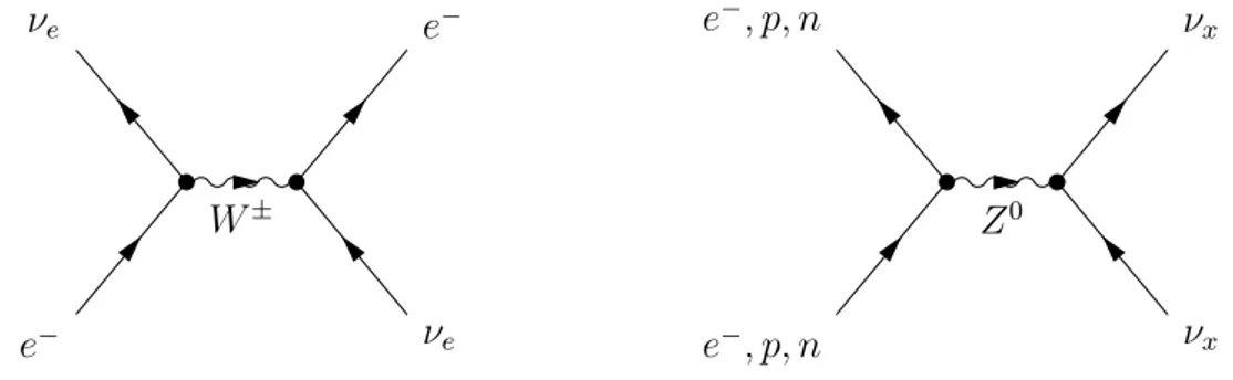
We consider CC and NC interactions of neutrinos with an unpolarized, electrically-neutral background of electrons, protons, and neutrons (see figure 2.4). While electron neutrinos can interact through both pro-cesses, muon and tau neutrinos are affected only by NC interactions.

W± e− νe νe e− Z0 e−, p, n νx e−, p, n νx

Figure 2.4:Feynman diagrams of the CC and NC interactions involved in the propagation of neutrino in a typical astrophysical environ-ment. The CC interactions (left) involves only electron neutrinos, while the NC interactions are avor blind: they can involve any neutrino

avor.

We derive the Γ

(−)

ν(ν−)_{matter contributions in the flavor basis, as, by definition, the matter interaction kernel}

is diagonal in this basis. We follow the procedure of section 2.2.2 in order to compute the CC contribution due to neutrino electron scattering

(33)

where ψeis the electron fermionic field, and the NC contribution T_NCµ (x) = ∑ f =e−,p,n ⟨_¯ ψf (x) γµ ( cf_v − v_afγ5 ) ψf(x) ⟩ , (2.74)

where the ψf are the fermionic field for particle f = e−, p, n. We assume that the background is

homoge-neous, and suppose that there are only forward and elastic scattering so that

ρf(t, ⃗p1, σ1, ⃗p2, σ2)≡ ⟨ a†_f (⃗p2, σ2) af(⃗p1, σ1) ⟩ = δσ1,σ2δ (3) (⃗p1− ⃗p2) ρf (t, ⃗p1) , (2.75)

with f = e−, p, n. Using the procedure of section 2.2.2 and trace techniques, we get for the CC interaction

T_CCµ (x) = 1 (2π)3 ∫ ⃗ p1,σ1 ¯ ue(⃗p1, σ1) γµ(1− γ5) ue(⃗p1, σ1) ρe(⃗p1, σ1) , (2.76) =− ∫ d3_p_⃗ e (2π)3 2ipµ e p0 e ρe(t, ⃗pe) , (2.77) ≡ −iJe,µ_, (2.78)

which gives the CC kernel, in the flavor basis

ΓCC_αβ = −iG√ F

2 γµ(1− γ5) J

e,µ_δ

αβδαe. (2.79)

The same computation can be done for the NC contribution (2.74), and we get

ΓNC_αβ = −iG√ F

2 γµ(1− γ5) ∑

f =e−,p,n

cf_vJf,µδαβ. (2.80)

Assuming that the background is electrically neutral, we have Je,µ _{= J}p,µ_{. We then use the value of the}

coefficients cf

v = I3− 2qfsin2θW and obtain

ΓNC_αβ = −iG√ F 2 γµ(1− γ5) ( −1 2J n,µ ) δαβ, (2.81)

which finally gives the entire matter contribution, adding Eqs. (2.79) and (2.81)

Γmat_αβ = −iG√ F 2 γµ(1− γ5) δαβ ( δαeJe,µ− 1 2J n,µ ) . (2.82)

Using the expression of the kernel and chiral spinor products A, introducing the notation ˆq = ⃗q_q, where

(34)

we obtain, for Dirac neutrinos

Γνν_ijmat(t, ⃗q, h, ⃗q′, h′) = δ(3)(⃗q− ⃗q′)[−δh,−δh,h′nµ(ˆq)· Σmatµ,ij

+δh,−h′ ( mj 2qδh,−e iϕ_ϵµ∗_(ˆ_{q) +}mi 2qδh,+e −iϕ_ϵµ_(ˆ_q) ) · Σmat µ,ij ] , (2.83)

Γν ¯_ij¯ν,mat(t, ⃗q, h, ⃗q′, h′) = δ(3)(⃗q− ⃗q′)[−δh,+δh,h′nµ(ˆq)· Σmatµ,ij

−δh,−h′ ( mj 2qδh,+e iϕ_ϵµ∗_(ˆ_{q) +} mi 2qδh,−e −iϕ_ϵµ_(ˆ_q) ) · Σmat µ,ij ] , (2.84)

Γν ¯_ijν,mat(t, ⃗q, h, ⃗q′, h′) = δ(3)(⃗q + ⃗q′)[−δh,−δh,−h′ϵµ∗(ˆq)· Σmatµ,ij

+δh,h′ ( mi 2qδh,+e −iϕ_nµ₍_{−ˆq) +}mj 2qδh,−e iϕ_nµ_(ˆ_q) ) Σmat_µ,ij ] , (2.85)

where Σ,ijmat,µis the matrix

Σmat,µ_αβ =√2GFδαβ ( δαeJe,µ− 1 2J n,µ ) , (2.86)

expressed in the mass basis. For Majorana neutrinos, we get

Γνν,_Mmat(t, ⃗q, h, ⃗q′, h′) = δ(3)(⃗q− ⃗q′)[δh,h′nµ(ˆq) ( −δh,−Σmatµ + δh,+Σmat,⊺µ ) +δh,−h′δh,+e−iϕϵµ(ˆq) ( m 2q · Σ mat µ + Σmat,µ ⊺· m 2q ) +δh,−h′δh,−eiϕϵµ∗(ˆq) ( Σmat_µ · m 2q + m 2q · Σ mat,⊺ µ )] , (2.87) Γν ¯_Mν,mat(t, ⃗q, h, ⃗q′, h′) = δ(3)(⃗q + ⃗q′)[δh,−h′ϵµ∗ ( −δh,−Σmatµ + δh,+Σmat,µ ⊺ ) (2.88) +δh,h′δh,+e−iϕ ( nµ(−ˆq) m 2q · Σ mat µ − n µ (ˆq) Σmat,⊺_µ · m 2q ) (2.89) +δh,h′δh,−eiϕ ( nµ(ˆq) Σmat_µ · m 2q − n µ (−ˆq) m 2q · Σ mat,⊺ µ )] , (2.90)