Second spectrum of Chromium (Cr II), Part II: Radiative lifetimes and oscillator strengths of transitions depopulating low lying 3d44p levels

(1)

Contents lists available at

ScienceDirect

Atomic Data and Nuclear Data Tables

journal homepage:

www.elsevier.com/locate/adt

Second spectrum of Chromium (Cr II), Part II: Radiative lifetimes and

oscillator strengths of transitions depopulating low lying 3d

4

4p levels

Safa Bouazza

a

,

*

, Pascal Quinet

b

,

c

, Patrick Palmeri

b

a_{Département de Physique, Université de Reims–Champagne, UFR SEN, BP 1039 F-51687 Reims Cedex2, France} b_{Physique Atomique et Astrophysique, Université de Mons-UMONS, B-7000 Mons, Belgium}

c_{IPNAS, Université de Liège, B-4000 Liège, Belgium}

a r t i c l e

i n f o

Article history:

Received 2 May 2017

Received in revised form 22 May 2017 Accepted 28 May 2017

Available online 20 June 2017

a b s t r a c t

Radiative lifetime and oscillator strength values were computed by means of a pseudo-relativistic

Hartree–Fock model including core-polarization and compared successfully with experimental data given

in the literature for respectively numerous low-lying Cr II 3d

4

_{4p levels, up to 54784 cm}

−1

_{, and transitions}

depopulating these levels. Then transition probability and branching fraction data were also deduced in

the wavelength range 1825–94400 Å. Furthermore the extracted radial integral values, obtained with the

help of the oscillator strength parameterization method, are given for involved transitions in this work,

i.e. 3d

4

_4s–3d

4

_{4p, 3d}

5

_–3d

4

_{4p and 3d}

4

_4p–3d

4

_{4d. We confirm our observed previous general trends, noting}

once again a decreasing of transition radial integral values with filling nd shells of the same principal

quantum numbers for nd

k

_(n

₊

_1)s

_→

_nd

k

_(n

₊

_{1)p transitions.}

© 2017 Elsevier Inc. All rights reserved.

*

Corresponding author.

E-mail address:safa.bouazza@univ-reims.fr(S. Bouazza).

http://dx.doi.org/10.1016/j.adt.2017.05.008

(2)

324 S. Bouazza et al. / Atomic Data and Nuclear Data Tables 120 (2018) 323–337

1. Introduction

... 324

2. Oscillator strength calculations

... 324

2.1. Some reminders

... 324

2.2. Lifetime considerations

... 325

2.3. Oscillator strength determination

... 325

2.4. Transition probability and branching fraction derivations

... 326

3. Conclusion

... 326

Acknowledgments

... 326

References

... 326

Explanation of Tables

... 327

Table 1.

Comparison between HFR+CPOL radiative lifetimes (in ns) and available experimental data for low-lying 3d

4

_{4p energy levels}

of Cr II.

... 327

Table 2.

Eigenvalue components of even-parity Cr II levels of interest in this study.

... 327

Table 3.

Eigenvalue components of odd-parity Cr II levels of interest in this study.

... 327

Table 4.

Comparison between experimental and calculated oscillator strength values.

... 327

Table 5.

Transition radial integral values in Cr II.

... 327

Table 6.

Semi-empirical radiative data in Cr II.

... 327

1. Introduction

The importance of accurate wavelengths and level energy

val-ues is now highly recognized in atomic physics when studying

hyperfine structure, isotope shifts, oscillator strengths or transition

probabilities of (sometimes blended) stellar spectral lines. It is

particularly difficult to disentangle the blends, in the case of the

elements of the 3d group due to their high relative abundance

and line-rich spectra. Fortunately now we have the chance to go

through high resolution spectra recorded with Fourier Transform

spectrometers (FTS) which have the potential to improve

signif-icantly the accuracy of the first-given wavelengths and then the

precision of energy levels by at least an order of magnitude. For

Cr II the most recent complete compilation of energy level data is

that of Sugar & Corliss [

1 ], based on the analysis of Kiess [

2 ] who

reported for the first time observations of spectra excited in direct

current arcs and condensed sparks between chromium electrodes.

The latter author succeeded in classifying 1843 lines linking 138

even-parity levels of 3d

5

_{, 3d}

4

_{4s and 3d}

3

_4s

2

_{configurations with}

139 3d

4

4p odd-parity levels. Johansson et al. [

3 ] extended the Kiess

study a half century later, particularly in the near-infrared region

and analyzed 450 additional levels. Sansonetti et al. [

4 –

6 ] reported

in turn new observations of Cr II some years later, in the

near-ultraviolet region 1140–3400 Å, and also up to the infrared region:

2850–37900 Å, using a 10.7 m normal incidence spectrograph

and an FT700 vacuum ultraviolet Fourier transform spectrometer.

These new measurements have been used to revise most of the Cr II

known levels [

5 –

8 ]. These reanalyzes have permitted to exchange

assignments of some levels classified in earlier lists of energy

levels, to shift positions of some quartets like 3d

4

5d

4

F

J

for instance

and to predict some still missing energy levels. In our previous

works, when determining radiative parameter values of some ions

we have observed as general trends a decreasing of transition

radial integral values with filling nd-shells of the same principal

quantum numbers for nd

k

_(n

₊

_1)s

_→

_nd

k

_(n

₊

_{1)p transitions.}

In the present work one of our aims is to extend the study of

transition radial integral behavior to another ion, located in the

same row of the periodic Table, namely Cr II, and by the way to

check our predicted transition radial integral value given in [

9 ]. To

extract this latter value we can take advantage of experimental

os-cillator strengths or transition probabilities, plentifully available in

literature [

10 –

14 ].

2. Oscillator strength calculations

2.1. Some reminders

We open this paragraph by reminding the reader of

impor-tant relations we have made use in this work, split in several

parts dealing each one with particular transitions: 3d

4

_4s–3d

4

_4p,

3d

4

_4p–3d

4

_{5s, 3d}

4

_4p–3d

4

_4d,

_{. . . .}

_{The oscillator strength f (}

_{γ γ}

′

) for

the transition between two levels

|

γ

J

⟩

and

|

γ

′

J

′

_⟩

of an atom or

molecule with statistical weights g

=

(2J

+

1) and g

′

₌

(2J

′

₊

1)

respectively, is a dimensionless physical quantity, expressing the

probability of absorption or emission in this transition between

these two levels and related to the transition probability W (

γ γ

′

)

by work [

15 ]

W (

γ γ

′

)

=

2 ω

2

_e

2

mc

2

f (

γ γ

′

)

(1)

where m and e are the electron mass and charge, c is the velocity

of light,

γ

describes the initial quantum state,

ω =

E(γ)−_h_¯E(γ′ )

, E(

γ

)

is the energy of the initial state. The quantities with primes refer

to the final state. For the electric dipole transitions, the weighted

oscillator strength gf is related to the line strength S [

15 ]

gf

=

8 π

2

mca

2₀

σ

3h

S

=

303 .

76 ×

10

−8

_σ

_S

₍₂₎

where a

0

is the Bohr radius,

σ =

E(γ)

−E(γ′ )

hc

and h is Planck’s

constant. The electric dipole line strength is defined by

S

= |⟨

γ

J

∥

P

1

∥

γ

′

J

′

⟩|

2

.

(3)

This quantity is a measure of the total strength of the spectral

line, including all possible transitions. The tensorial operator P

1

(first order) given in units of ea

0

in the reduced matrix element

stands for the electric dipole moment. To obtain the gf value,

we need to calculate initially S, or preferably its square root. For

multiconfiguration systems, the wavefunctions

|

γ

J

⟩

and

|

γ

′

J

′

_⟩

are

expanded in terms of a set of basis functions

|

φ

SLJ

⟩

and

|

φ

′

S

′

L

′

J

′

_⟩

,

respectively

|

γ

J

⟩ =

∑

i

c

i

|

φ

i

S

i

L

i

J

⟩

|

γ

′

J

′

⟩ =

∑

j

c

′ j

|

φ

′ j

S

′ j

L

′ j

J

′

⟩

.

(4)

(3)

The square root of the line strength may be written in the following

form

S

_{γ γ}1/2′

=

∑

i

∑

j

c

i

c

j

⟨

φ

i

S

i

L

i

J

∥

P

1

∥

φ

′ j

S

′ j

L

′ j

J

′

⟩

.

(5)

In this work we have recurred to the eigenvector amplitudes

ob-tained by a parametric analysis of multiconfiguration systems of

Cr II reported in our previous paper [

8 ].

The even system contains 11 configurations: 3d

5

_{+ 3d}

4

_{ns (n}

₌

4 −

9) + 3d

4

_n

′

d (n

′

₌

4 −

6) + 3d

3

_4s

2

_{, and the odd system contains}

6 configurations: 3d

4

_{4p + 3d}

4

_{5p + 3d}

4

_{6p + 3d}

3

_{4s4p + 3d}

4

_{4f + 3d}

4

_5f.

The appropriate computer program [

16 ] calculates the angular part

of the matrix element

⟨

φ

SLJ

∥

P

1

∥

φ

′

S

′

L

′

J

′

⟩

. From Eqs.

(2)

and

(5)

, we

can express the gf -values as a linear combination

(gf )

1/2

=

∑

nl,n′l′

(303

.

76 ×

10

−8

σ

)

1/2

×

∑

i

∑

j

c

i

c

j′

⟨

φ

i

S

i

L

i

J

∥

P

1

∥

φ

′j

S

′ j

L

′ j

J

′

⟩

(6)

where

σ

is the wavenumber, given in cm

−1

_{, and the sum extends}

over all possible transitions (ns

↔

n

′

p, nd

↔

n

′

p, nd

↔

n

′

f). The

probability per unit time of an atom in a specific state

γ

J to make

a spontaneous transition to any state with lower energy is P(

γ

J)

=

∑

A(

γ

J

, γ

′

J

′

), where A(

γ

J

, γ

′

J

′

) is the Einstein spontaneous

emis-sion transition probability rate for a transition from

γ

J to

γ

′

J

′

states. The sum is over all

γ

′

J

′

states with E(

γ

′

J

′

)

<

E(

γ

J).

The weighted transition probability is [

17 ]

gA

=

(2J

′

+

1)A

=

64 π

4

_e

2

_a

0

3h

σ

3

_S

₌

₂

_.

₀₂₆₁

_×

₁₀

−6

_σ

3

_S

₍₇₎

where

σ

is given, as previously, in cm

−1

_{and S in atomic units of}

e

2

_a

2

0

. Substitution of Eq.

(2)

into

(7)

leads to

(2J

′

+

1)A

=

0 .

66702

σ

2

gf

.

(8)

To determine the branching fractions it is necessary to measure

the lifetime of the upper level in the case of emission or the

lifetime of the lower level in the case of absorption, as well as

the relative intensities of all lines originating from the considered

level. The branching fraction, BF , is defined in the case of emission,

appropriate to experimental data of interest here, as

BF

ul

=

A

ul

∑

k

A

uk

=

_∑

I

ul k

I

uk

(9)

with u standing for the upper and l the lower levels. The lifetime,

τ

, is defined as the inverse of the probability

τ

u

=

1 ∑

k

A

uk

.

(10)

Using Eqs.

(9)

and

(10)

one obtains

BF

ul

=

A

ul

×

τ

u

.

(11)

2.2. Lifetime considerations

Engman et al. [

18 ] and Pinnington et al. [

19 ] have used the

beam-foil technique to measure radiative lifetimes of low-lying

levels of the Cr II 3d

4

(

5

D)4p configuration. Later Schade et al. [

20 ],

Pinnington et al. [

14 ], Bergeson and Lawler [

10 ] and Nilsson

et al. [

11 ] have extended these experimental data using the

time-resolved laser-induced fluorescence method. The latter technique

has been improved by the use of a frequency-doubled

distributed-feedback dye laser which is directly pumped by a part of a

XeCl-excimer laser beam. These data are shown in

Table 1

.

2.3. Oscillator strength determination

To evaluate line strengths we have recourse to Eq.

(5)

. As in

previous works devoted to oscillator strength determination (see

for instance [

27 ]), the angular coefficients of the transition matrix,

obtained in pure SL coupling with the help of Racah algebra is

transformed into the actual intermediate coupling pertaining to

our level eigenvector amplitudes, Moreover the transition integrals

∫

∞

0

P

nl

(r)rP

n′l′

(r)dr

(12)

are treated as free parameters in the least squares fit to

experimen-tal gf values. As we proceeded previously we have first sorted out

the strongest lines, not blended, and particularly those

represent-ing transitions between levels with a limited number of leadrepresent-ing

components, displayed in their entirety for the reader in

Tables 2

and

3 (up to 0.005%). With the combination of time-resolved

laser induced fluorescence radiative lifetime determinations and

FTS branching fraction measurements, Nilsson et al. [

11 ] have

generated a complete set of gf -values in the wavelength range

2050–4850 Å with an uncertainty varying from 3% to 42%. From

these Cr II 3d

4

_4s–3d

4

_{4p transitions we have selected in a first stage}

only those depopulating low-lying 3d

4

_{4p levels (the highly excited}

levels will be considered in another paper). The comparison of 119

improved experimental [

11 ] and calculated oscillator strengths of

these selected transitions (including 94 fitted values) is presented

in

Table 4

. In the latter, we additionally have inserted some other

data found in the literature. For most transitions, the observed and

calculated oscillator strength values are very consistent within the

experimental accuracy. Then we have extracted semi-empirically,

with a very good accuracy the transition radial integral values,

re-ported in

Table 5

. In this table we have inserted also the transition

radial integral value of 3d

4

_4p–3d

4

_{4d, admittedly with less good}

accuracy since we have rooted out only the 3d

4

_{4d contributions to}

3d

4

_{4s levels. Let us point out that the obtained}

_⟨

_3d

4

_4s

_|

_r

1

_|

_3d

4

_4p

_{⟩ =}

2 .

932(0

.

003) is very close to the predicted value reported in our

previous work [

9 ], i.e. 3.00 (0.02). In the same table, we also give

the results computed by means of the pseudo-relativistic Hartree–

Fock (HFR) method using the basic Cowan code [

17 ], on the one

hand, and including core-polarization (HFR+CPOL), as described

in [

21 ,

22 ], on the other hand. As a reminder, in the latter approach,

the radial dipole integrals given in Eq.

(12)

are replaced by

∫

∞ 0

P

nl

(r)r

[

1 −

α

d

(r

2

₊

_r

2 c

)

3/2

]

P

n′l′

(r)dr

−

α

d

r

3 c

∫

rc 0

P

nl

(r)rP

n′l′

(r)dr

(13)

where

α

d

is the dipole polarizability of the ionic core, for which

numerical values can be found in the literature (see e.g. [

23 ]),

and r

c

is the cut-off radius that is arbitrarily chosen as a

mea-sure of the size of the ionic core. In practice, this

parame-ter is usually chosen to be equal to the HFR mean value

⟨

r

⟩

for the outermost ionic core orbital. In the present work, the

HFR+CPOL approach was used with a Cr IV ionic core (

α

d

=

1 .

96a

3

0

[

23 ]; r

c

=

1 .

20a

0

) in addition to the explicit

considera-tion of the following interacting configuraconsidera-tions: 3d

5

_{, 3d}

4

_{4s, 3d}

4

_5s,

3d

4

_{6s, 3d}

4

_{4d, 3d}

4

_{5d, 3d}

4

_{6d, 3d}

3

_4s

2

_{, 3d}

3

_4p

2

_{, 3d}

3

_4d

2

_{, 3d}

3

_4s4d,

3d

3

_{4s5s for the even parity, and 3d}

4

_{4p, 3d}

4

_{5p, 3d}

4

_{6p, 3d}

4

_4f,

3d

4

_{5f, 3d}

4

_{6f, 3d}

3

_{4s4p, 3d}

3

_{4s4f, 3d}

3

_{4p4d for the odd parity.}

Moreover, this HFR+CPOL model was combined with a

well-established semi-empirical adjustment of the radial parameters

in order to minimize the discrepancies between the calculated

energy levels and the available experimental values [

1 –

7 ] up

to 105000 cm

−1

. In

Table 1

, the radiative lifetimes obtained

with this method are compared with the experimental data for

the low-lying 3d

4

_{4p energy levels. As seen from this table a}

very good agreement is observed, the mean ratio

τ

HFR+CPOL

/τ

exp

(4)

resulting to 0.96

±

0.04 when considering the two sets of

experimental lifetime values due to Schade et al. [

20 ] and Nilsson

et al. [

11 ].

2.4. Transition probability and branching fraction derivations

After having considered the radiative lifetimes, the oscillator

strengths and transition radial integrals, we propose to close this

study by computing the transition probabilities and branching

fractions for all transitions depopulating the low-lying 3d

4

_{4p levels}

(lower than 54785 cm

−1

_{) and whose log(gf )}

_{≥ −}

_{4, using HFR}

+ CPOL model and to compare them with semi-empirical data of

Kurucz [

24 ]. All these data are reported in

Table 6

from which

a rather fairly good agreement can be observed for transitions

covering a wide wavelength range, from 2344 to 7580 Å.

3. Conclusion

We have extended our previous studies concerning oscillator

strengths to another singly ionized atom: Cr II. In the whole our

semi-empirical calculations agree well with experimental data

within the uncertainty of measurements found in the literature.

Our predictions for Cr II transition radial integral values have

turned out favorably thanks to this work and now we can consider

as a law what we previously consider only as general trends, seeing

the large number of recognized cases: a decreasing of transition

radial integral values with filling nd-shells of the same principal

quantum numbers for nd

k

_(n

₊

_1)s

_→

_nd

k

_(n

₊

_{1)p transitions.}

We will check again these values in the near future since we plan

to compute the gf-values of transitions depopulating higher Cr II

levels than those considered in the present work.

Acknowledgments

PQ and PP are respectively Research Director and Research

Associate of the Belgian Fund for Scientific Research F.R.S.-FNRS.

Financial support from this organization is deeply acknowledged.

References

[1] J. Sugar, C. Corliss, J. Phys. Chem. Ref. Data Suppl. 14 (1985) 264.

[2] C.C. Kiess, J. Res. Nat. Bur. Std. 60 (1958) 375 RP2856.

[3] S. Johansson, T. Zethson, H. Hartman, et al., Astron. Astrophys. 361 (2000) 977.

[4] C.J. Sansonetti, F. Kerber, J. Reader, M.R. Rosa, Astrophys. J. Suppl. Series 153 (2004) 555.

[5] C.J. Sansonetti, G. Nave, J. Reader, F. Kerber, Astrophys. J Suppl. Series 202 (2012) 15.

[6] C.J. Sansonetti, G. Nave, Astrophys. J. Suppl. Series 213 (2014) 1.

[7] E.B. Saloman, J. Phys. Chem. Ref. Data 41 (2012) 043103.

[8] S. Bouazza, P. Quinet, P. Palmeri, (ADNDT), accepted,http://dx.doi.org/10. 1016/j.adt.201705003.

[9] S. Bouazza, P. Quinet, P. Palmeri, J. Quant. Spectrosc. Radiat. Transf. 199 (2017) 66.

[10]S.D. Bergeson, J.E. Lawler, Astrophys. J. 408 (1993) 382.

[11]H. Nilsson, G. Lyung, H. Lundberg, K.E. Nielsen, Astron. Astrophys. 445 (2006) 1165.

[12]J. Musielok, T. Wujec, Astron. Astrophys. Suppl. Series 38 (1979) 119.

[13]J. Gurell, H. Nilsson, L. Engström, H. Lundberg, R. Blackwell-Whitehead, K.E. Nielsen, S. Mannervik, Astron. Astrophys. 511 (2010) A68.

[14]E.H. Pinnington, Q. Ji, B. Gou, et al., Can. J. Phys. 71 (1993) 470.

[15]I. Sobelman, Atomic Spectra and Radiative Transitions, Springer-Verlag, Berlin, 1978.

[16]J. Ruczkowski, M. Elantkowska, J. Dembczynski, J. Quant. Spectrosc. Radiat. Transf. 145 (2014) 20.

[17]R.D. Cowan, The Theory of Atomic Structure Spectra, University of California Press, Berkeley, CA, 1981.

[18]B. Engman, A. Gaupp, L.J. Curtis, I. Martinson, Phys. Scr. 12 (1975) 220.

[19]E.H. Pinnington, H.O. Lutz, G.W. Carriaveao, Nucl. Instrum. Methods 110 (1973) 55.

[20]W. Schade, B. Mundt, V. Helbig, Phys. Rev. A 42 (1990) 3.

[21]P. Quinet, P. Palmeri, E. Biémont, M.M. McCurdy, G. Rieger, E.H. Pinnington, M.E. Wickliffe, J.E. Lawler, Mon. Not. R. Astron. Soc. 307 (1999) 934.

[22]P. Quinet, P. Palmeri, E. Biémont, Z.S. Li, Z.G. Zhang, S. Svanberg, J. Alloys Compd. 344 (2002) 255.

[23]S. Fraga, J. Karwowski, K.M.S. Saxena, Handbook of Atomic Data, Elsevier Scientific Publishing Company, Amsterdam, 1976.

[24] R.L. Kurucz (1995), Atomic spectral line data from CD-ROM Nr. 23,http://www. cfa.harvard.edu/amp/ampdata/kurucz23/sekur.html.

[25]R. Spreger, B. Schelm, M. Kock, T. Neger, M. Ulbel, J. Quant. Spectrosc. Radiat. Transf. 51 (1994) 779.

[26]A.M. Gonzalez, M. Ortiz, J. Compos, Can. J. Phys. 72 (1994) 57.

[27]J. Ruczkowski, S. Bouazza, M. Elantkowska, J. Dembczynski, J. Quant. Spectrosc. Radiat. Transf. 155 (2015) 1.

(5)

Explanation of Tables

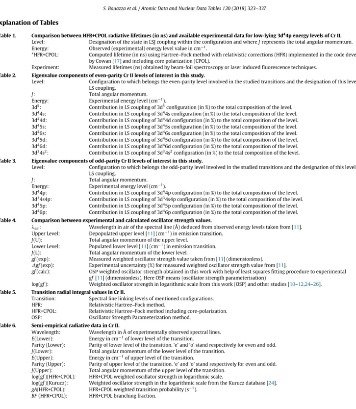
Table 1. Comparison between HFR+CPOL radiative lifetimes (in ns) and available experimental data for low-lying 3d4_{4p energy levels of Cr II.}

Level: Designation of the state in LSJ coupling within the configuration and where J represents the total angular momentum. Energy: Observed (experimental) energy level value in cm−1_.

*HFR+CPOL: Computed lifetime (in ns) using Hartree–Fock method with relativistic corrections (HFR) implemented in the code developed by Cowan [17] and including core polarization (CPOL).

Experiment: Measured lifetimes (ns) obtained by beam-foil spectroscopy or laser induced fluorescence techniques.

Table 2. Eigenvalue components of even-parity Cr II levels of interest in this study.

Level: Configuration to which belongs the even-parity level involved in the studied transitions and the designation of this level in LS coupling.

J: Total angular momentum. Energy: Experimental energy level (cm−1_).

3d5_: _{Contribution in LS coupling of 3d}5_{configuration (in %) to the total composition of the level.}

3d4_4s: _{Contribution in LS coupling of 3d}4_{4s configuration (in %) to the total composition of the level.}

3d4_4d: _{Contribution in LS coupling of 3d}4_{4d configuration (in %) to the total composition of the level.}

3d3_4s2_: _{Contribution in LS coupling of 3d}3_4s2_{configuration (in %) to the total composition of the level.}

Table 3. Eigenvalue components of odd-parity Cr II levels of interest in this study.

Level: Configuration to which belongs the odd-parity level involved in the studied transitions and the designation of this level in LS coupling.

J: Total angular momentum. Energy: Experimental energy level (cm−1_).

3d4_4p: _{Contribution in LS coupling of 3d}4_{4p configuration (in %) to the total composition of the level.}

3d3_4s4p: _{Contribution in LS coupling of 3d}3_{4s4p configuration (in %) to the total composition of the level.}

Table 4. Comparison between experimental and calculated oscillator strength values.

λ

air: Wavelength in air of the spectral line (Å) deduced from observed energy levels taken from [11].

Upper Level: Depopulated upper level [11] (cm−1_{) in emission transition.} J(U): Total angular momentum of the upper level.

Lower Level: Populated lower level [11] (cm−1_{) in emission transition.} J(L): Total angular momentum of the lower level.

gf (exp): Measured weighted oscillator strength value taken from [11] (dimensionless).

∆

gf (exp): Experimental uncertainty (%) for measured weighted oscillator strength value from [11].

gf (calc): OSP weighted oscillator strength obtained in this work with help of least squares fitting procedure to experimental

gf [11] (dimensionless). Here OSP means (oscillator strength parameterisation)

log(gf ): Weighted oscillator strength in logarithmic scale from this work (OSP) and other studies [10–12,24–26].

Table 5. Transition radial integral values in Cr II.

Transition: Spectral line linking levels of mentioned configurations. HFR: Relativistic Hartree–Fock method.

HFR+CPOL: Relativistic Hartree–Fock method including core-polarization. OSP: Oscillator Strength Parameterization method.

Table 6. Semi-empirical radiative data in Cr II.

Wavelength: Wavelength in Å of experimentally observed spectral lines.

E(Lower): Energy in cm−1_{of lower level of the transition.}

Parity (Lower): Parity of lower level of the transition. ‘e’ and ‘o’ stand respectively for even and odd.

J(Lower): Total angular momentum of the lower level of the transition.

E(Upper): Energy in cm−1_{of upper level of the transition.}

Parity (Upper): Parity of upper level of the transition. ‘e’ and ‘o’ stand respectively for even and odd.

J(Upper): Total angular momentum of the upper level of the transition. log(gf )(HFR+CPOL): HFR+CPOL weighted oscillator strength in logarithmic scale.

log(gf )(Kurucz): Weighted oscillator strength in the logarithmic scale from the Kurucz database [24].

gA(HFR+CPOL): HFR+CPOL weighted transition probability (s−1_). BF (HFR+CPOL): HFR+CPOL branching fraction.

(6)

Table 1

Comparison between HFR+CPOL radiative lifetimes (in ns) and available experimental data for low-lying 3d4_{4p energy}

levels of Cr II.

Level Energy HFR+CPOL Experiment

(cm−1₎ _{Ref. [}₁₁_] _{Ref. [}₂₀_] _{Refs. [}₁₄_,₁₉_] _{Ref. [}₁₀_] _{Ref. [}₁₈_] 6_F 1/2 46824 4.2 4.3(1) 6_F 3/2 46906 4.1 4.2(1) 6_F 5/2 47041 4.1 4.2(1) 6_F 7/2 47228 4.1 4.1(1) 6_F 9/2 47465 4.1 4.2(1) 6_F 11/2 47752 4.0 4.0(1) 6_P 3/2 48399 2.2 2.4(1) 6_P 5/2 48491 2.2 2.3(2) 2.5(1) 2.45 2.4(2) 3.2(4) 6_P 7/2 48632 2.2 2.4(2) 2.5(1) 2.40(13) 2.4(2) 3.3(4) 4_P 1/2 48750 4.8 5.0(2) 4_P 3/2 49006 4.7 4.7(2) 4_P 5/2 49352 4.3 4.6(2) 6_D 1/2 49493 3.8 4.3(2) 6_D 3/2 49565 3.9 4.2(1) 6_D 7/2 49646 3.6 3.8(1) 6_D 5/2 49706 4.1 4.5(1) 6_D 9/2 49838 3.6 3.8(2) 4_F 3/2 51584 4.2 4.2(4) 4_F 5/2 51669 4.2 4.1(4) 4_F 7/2 51789 4.2 4.1(3) 4_F 9/2 51943 4.2 4.1(3) 4_D 1/2 54418 4.1 4.3(4) 4_D 3/2 54500 4.1 4.3(4) 4_D 5/2 54626 4.1 4.3(4) 4_D 5/2 54784 4.1 4.3(4) 4.20(18) Table 2

Eigenvalue components of even-parity Cr II levels of interest in this study.

Level J Energy 3d5 _3d4_4s _3d4_4d _3d4_5s _3d4_6s _3d4_5d _3d4_6d _3d3_4s2 (cm−1₎ _(%) _(%) _(%) _(%) _(%) _(%) _(%) _(%) 3d4_{4s a}6_D _1/2 ₁₁₉₆₂ _99.93 _0.02 _0.03 3d4_{4s a}4_D _1/2 ₁₉₅₂₈ _4.36 _95.35 _0.16 _0.02 _0.03 _0.01 3d5_a4_P _1/2 ₂₁₈₂₄ _97.21 _1.39 _0.69 _0.02 _0.17 _0.06 _0.43 3d4_{4s a}6_D _3/2 ₁₂₀₃₃ _99.93 _0.02 _0.03 3d4_{4s a}4_D _3/2 ₁₉₆₃₁ _4.36 _95.08 _0.16 _0.06 _0.02 _0.03 _0.01 3d5_a4_P _3/2 ₂₁₈₂₄ _97.21 _1.43 _0.69 _0.02 _0.17 _0.06 _0.42 3d5_a6_S _5/2 ₀ _99.91 _0.01 _0.06 _0.01 3d4_{4s a}6_D _5/2 ₁₂₁₄₈ _99.93 _0.02 _0.03 3d4_{4s a}4_D _5/2 ₁₉₇₉₈ _4.99 _94.72 _0.17 _0.06 _0.02 _0.03 _0.01 3d5_a4_G _5/2 ₂₀₅₁₂ _98.99 _0.40 _0.39 _0.01 _0.16 _0.05 3d5_a4_P _5/2 ₂₁₈₂₃ _97.26 _1.39 _0.69 _0.02 _0.17 _0.42 3d4_{4s a}6_D _7/2 ₁₂₃₀₄ _99.93 _0.02 _0.03 3d4_{4s a}4_D _7/2 ₂₀₀₂₄ _5.17 _94.53 _0.17 _0.06 _0.02 _0.03 _0.01 3d5_a4_G _7/2 ₂₀₅₁₈ _99.00 _0.40 _0.39 _0.01 _0.15 _0.05 3d4_{4s a}6_D _9/2 ₁₂₄₉₆ _99.93 _0.02 _0.03 3d5_a4_G _11/2 ₂₀₅₁₂ _99.02 _0.38 _0.38 _0.01 _0.15 _0.05

(7)

Table 3

Eigenvalue components of odd-parity Cr II levels of interest in this study.

Level J Energy 3d4_4p _3d3_4s4p _3d4_5p _3d4_6p (cm−1₎ _(%) _(%) _(%) _(%) z6_F _1/2 ₄₆₈₂₃ _99.57 _0.10 _0.27 _0.06 z4_P _1/2 ₄₈₇₄₉ _99.62 _0.22 _0.12 _0.03 z6_D _1/2 ₄₉₄₉₃ _99.52 _0.31 _0.13 _0.02 z4_D _1/2 ₅₄₄₁₈ _99.48 _0.37 _0.11 _0.03 z6_F _3/2 ₄₆₉₀₅ _99.57 _0.10 _0.27 _0.06 z6_P _3/2 ₄₈₃₉₉ _99.74 _0.13 _0.09 _0.03 z4_P _3/2 ₄₉₀₀₆ _99.62 _0.23 _0.12 _0.03 z6_D _3/2 ₄₉₅₆₅ _99.52 _0.31 _0.13 _0.02 z4_D _3/2 ₅₄₄₉₉ _99.49 _0.37 _0.11 _0.03 z6_F _5/2 ₄₇₀₄₀ _99.57 _0.10 _0.27 _0.06 z6_P _5/2 ₄₈₃₉₁ _99.74 _0.13 _0.09 _0.03 z6_D _5/2 ₄₉₃₅₂ _99.59 _0.26 _0.13 _0.03 z4_P _5/2 ₄₉₇₀₆ _99.56 _0.28 _0.13 _0.02 z6_F _7/2 ₄₇₂₂₇ _99.57 _0.10 _0.27 _0.06 z6_P _7/2 ₄₈₆₃₂ _99.74 _0.13 _0.09 _0.03 z6_D _7/2 ₄₉₆₄₆ _99.49 _0.35 _0.14 _0.02 z4_F _7/2 ₅₁₇₈₉ _99.74 _0.14 _0.09 _0.02 z4_D _7/2 ₅₄₇₈₄ _99.49 _0.36 _0.11 _0.03 z6_F _9/2 ₄₇₄₆₅ _99.57 _0.10 _0.27 _0.06 z6_D _9/2 ₄₉₈₃₈ _99.49 _0.34 _0.14 _0.02 z4_F _9/2 ₅₁₉₄₃ _99.74 _0.14 _0.09 _0.02

(8)

330 S. Bouazza et al. / Atomic Data and Nuclear Data Tables 120 (2018) 323–337 Table 4

Comparison between experimental and calculated oscillator strength values.

λ

air Upper Level J(U) Lower Level J(L) gf (exp)

∆

gf (exp) gf (calc) log(gf )

(Å) (cm−1₎ _(cm−1₎ _(%) _[₁₁_] _OSP _[₂₄_] _[₂₅_] _[₁₀_] _[₂₆_] _[₁₂_] 2531.85 51788.816 7/2 12303.82 7/2 0.0182 12 0.0106

−

1.740

−

1.9756

−

1.878 2534.33 51942.664 9/2 12496.456 9/2 0.0484 12 0.0345

−

1.315

−

1.4616

−

1.361 2653.58 49706.262 5/2 12032.545 3/2 0.2415 6 0.4034

−

0.617

−

0.3943

−

0.304 2658.59 49564.504 3/2 11961.747 1/2 0.2642 8 0.3447

−

0.578

−

0.4626

−

0.45 2661.72 49706.262 5/2 12147.772 5/2 0.0728 6 0.1355

−

1.138

−

0.8681

−

0.755 2663.42 49838.379 9/2 12303.82 7/2 0.561 40 0.633

−

0.251

−

0.1986

−

0.205 2663.60 49564.504 3/2 12032.545 3/2 0.0238 9 0.0049

−

1.623

−

2.3056

−

2.181 2663.67 49492.711 1/2 11961.747 1/2 0.0912 8 0.1127

−

1.040

−

0.9480

−

0.973 2666.01 49645.805 7/2 12147.772 5/2 0.7834 23 0.8761

−

0.106

−

0.0574

−

0.064

−

0.1

−

0.056

−

0.313 2668.71 49492.711 1/2 12032.545 3/2 0.3097 8 0.3863

−

0.509

−

0.4131

−

0.448

−

0.67

−

0.537

−

0.557 2671.81 49564.504 3/2 12147.772 5/2 0.4667 7 0.5881

−

0.331

−

0.2306

−

0.271

−

0.34

−

0.373

−

0.377 2672.83 49706.262 5/2 12303.82 7/2 0.369 6 0.5366

−

0.433

−

0.2703

−

0.281

−

0.59

−

0.468 2678.79 49351.734 5/2 12032.545 3/2 0.5176 7 0.4382

−

0.286

−

0.3583

−

0.475

−

0.39

−

0.351 2687.09 49351.734 5/2 12147.772 5/2 0.2786 7 0.2565

−

0.555

−

0.5908

−

0.674

−

0.6

−

0.608 2691.04 49645.805 7/2 12496.456 9/2 0.4446 23 0.5079

−

0.352

−

0.2942

−

0.403

−

0.337 2698.41 49351.734 5/2 12303.82 7/2 0.2871 8 0.1931

−

0.542

−

0.7143

−

1.077 2698.68 49005.848 3/2 11961.747 1/2 0.2729 6 0.2362

−

0.564

−

0.6268

−

0.656 2703.85 49005.848 3/2 12032.545 3/2 0.0406 7 0.043

−

1.392

−

1.3664

−

1.327 2712.31 49005.848 3/2 12147.772 5/2 0.159 6 0.106

−

0.799

−

0.9746

−

1.167

−

0.76 2717.51 48749.277 1/2 11961.747 1/2 0.0372 8 0.0308

−

1.430

−

1.5121

−

1.543 2722.75 48749.277 1/2 12032.545 3/2 0.1361 6 0.1077

−

0.866

−

0.9678

−

1.014

−

1.002 2740.10 48632.059 7/2 12147.772 5/2 0.0798 12 0.081

−

1.098

−

1.0917

−

1.233

−

1.18

−

1.09

−

1.091

−

1.004 2742.03 48491.059 5/2 12032.545 3/2 0.2042 9 0.1945

−

0.690

−

0.7111

−

0.817

−

0.82

−

0.68

−

0.626 2743.64 48398.871 3/2 11961.747 1/2 0.3459 9 0.3349

−

0.461

−

0.4751

−

0.545

−

0.47

−

0.47 2748.98 48398.871 3/2 12032.545 3/2 0.527 9 0.5378

−

0.278

−

0.2694

−

0.305

−

0.52

−

0.28

−

0.257 2750.73 48491.059 5/2 12147.772 5/2 0.6501 9 0.6714

−

0.187

−

0.1730

−

0.226

−

0.43

−

0.18

−

0.199 2751.86 48632.059 7/2 12303.82 7/2 0.5058 9 0.5286

−

0.296

−

0.2769

−

0.349

−

0.69

−

0.29

−

0.294 2757.73 48398.871 3/2 12147.772 5/2 0.455 9 0.4463

−

0.342

−

0.3504

−

0.349

−

0.53

−

0.36

−

0.372 2762.59 48491.059 5/2 12303.82 7/2 1.0914 9 1.1292 0.038 0.0528 0.048

−

0.28 0.05 0.024 2766.53 48632.059 7/2 12496.456 9/2 2.0512 9 2.1053 0.312 0.3233 0.31 0.32 0.301 2835.63 47751.602 11/2 12496.456 9/2 3.6141 3 3.8391 0.558 0.5842 0.572 0.562 2849.83 47227.219 7/2 12147.772 5/2 1.4852 3 1.6041 0.171 0.2052 0.184 0.13 0.15

−

0.067 2855.67 47040.273 5/2 12032.545 3/2 0.8299 4 0.8964

−

0.081

−

0.0475

−

0.069

−

0.18

−

0.101 2856.76 54625.594 5/2 19631.205 3/2 0.241 10 0.3301

−

0.618

−

0.4813

−

0.598

−

0.71

−

0.511 2857.40 54784.449 7/2 19797.859 5/2 0.2061 11 0.2549

−

0.686

−

0.5937

−

0.698

−

0.562 2858.65 54499.492 3/2 19528.23 1/2 0.1832 11 0.25

−

0.737

−

0.6021

−

0.726 2858.91 47464.559 9/2 12496.456 9/2 0.597 6 0.6208

−

0.224

−

0.2071

−

0.196

−

0.179 2860.93 46905.137 3/2 11961.747 1/2 0.3556 5 0.3882

−

0.449

−

0.4110

−

0.432

−

0.503

−

0.49 2862.57 47227.219 7/2 12303.82 7/2 0.8511 5 0.8844

−

0.070

−

0.0534

−

0.053

−

0.45

−

0.034

−

0.229 2865.10 47040.273 5/2 12147.772 5/2 0.8166 4 0.8906

−

0.088

−

0.0503

−

0.057

−

0.12

−

0.045 2865.33 54417.957 1/2 19528.23 1/2 0.1901 11 0.2799

−

0.721

−

0.5530

−

0.688 2867.09 54499.492 3/2 19631.205 3/2 0.3251 10 0.4636

−

0.488

−

0.3339

−

0.474

−

0.266 2867.65 46823.305 1/2 11961.747 1/2 0.4365 3 0.4902

−

0.360

−

0.3096

−

0.324

−

0.353

−

0.567 2873.48 46823.305 1/2 12032.545 3/2 0.138 6 0.1417

−

0.860

−

0.8486

−

0.853

−

0.843 2873.81 54417.957 1/2 19631.205 3/2 0.2104 11 0.2965

−

0.677

−

0.5279

−

0.662

−

0.672 2875.99 54784.449 7/2 20024.012 7/2 1.531 10 2.0221 0.185 0.3058 0.175 2876.24 46905.137 3/2 12147.772 5/2 0.1462 5 0.155

−

0.835

−

0.8096

−

0.804

−

0.58 2878.44 47227.219 7/2 12496.456 9/2 0.0481 8 0.0499

−

1.318

−

1.3016

−

1.27

−

1.304

−

1.158 2880.86 54499.492 3/2 19797.859 5/2 0.317 10 0.4369

−

0.499

−

0.3596

−

0.493

−

0.411 2889.19 54625.594 5/2 20024.012 7/2 0.278 10 0.3752

−

0.556

−

0.4258

−

0.554 3032.92 54784.449 7/2 21822.506 5/2 0.0486 20 0.0959

−

1.313

−

1.0183

−

1.031 3047.61 54625.594 5/2 21824.141 3/2 0.0263 21 0.0535

−

1.580

−

1.2717

−

1.326 3118.65 51584.102 3/2 19528.23 1/2 0.7907 10 0.6897

−

0.102

−

0.1613

−

0.081

−

0.004 (continued on next page)

(9)

S. Bouazza et al. / Atomic Data and Nuclear Data Tables 120 (2018) 323–337 331

λ

air Upper Level J(U) Lower Level J(L) gf (exp)

∆

gf (exp) gf (calc) log(gf )

(Å) (cm−1₎ _(cm−1₎ _(%) _[₁₁_] _OSP _[₂₄_] _[₂₅_] _[₁₀_] _[₂₆_] _[₁₂_] 3124.98 51788.816 7/2 19797.859 5/2 1.932 8 1.6578 0.286 0.2195 0.303 0.44 3128.70 51584.102 3/2 19631.205 3/2 0.2965 11 0.2452

−

0.528

−

0.6105

−

0.511

−

0.82

−

0.362 3132.05 51942.664 9/2 20024.012 7/2 2.7353 7 2.308 0.437 0.3632 0.451 0.57 3136.69 51669.406 5/2 19797.859 5/2 0.3855 11 0.2978

−

0.414

−

0.5260

−

0.416

−

0.29

−

0.254 3147.22 51788.816 7/2 20024.012 7/2 0.2965 9 0.2087

−

0.528

−

0.6805

−

0.558

−

0.18 3180.69 51942.664 9/2 20512.098 11/2 0.6383 9 0.4372

−

0.195

−

0.3593

−

0.131 3209.18 51669.406 5/2 20517.793 7/2 0.3882 11 0.2476

−

0.411

−

0.6063

−

0.372

−

0.214 3217.40 51584.102 3/2 20512.062 5/2 0.2704 11 0.1831

−

0.568

−

0.7373

−

0.501

−

0.332 3324.06 49706.262 5/2 19631.205 3/2 0.0296 14 0.0216

−

1.529

−

1.6648

−

1.691

−

1.21 3328.35 49564.504 3/2 19528.23 1/2 0.0196 22 0.0156

−

1.708

−

1.8067

−

1.752 3336.33 49492.711 1/2 19528.23 1/2 0.0673 14 0.0495

−

1.172

−

1.3054

−

1.172 3339.80 49564.504 3/2 19631.205 3/2 0.1057 13 0.0762

−

0.976

−

1.1182

−

1.044

−

1.03 3342.58 49706.262 5/2 19797.859 5/2 0.1545 6 0.1081

−

0.811

−

0.9660

−

1.03

−

0.51 3347.83 49492.711 1/2 19631.205 3/2 0.0705 14 0.046

−

1.152

−

1.3371

−

1.17

−

1.24 3353.12 49838.379 9/2 20024.012 7/2 0.0244 42 0.0203

−

1.613

−

1.6918

−

1.477

−

0.97 3358.50 49564.504 3/2 19797.859 5/2 0.2143 13 0.1399

−

0.669

−

0.8543

−

0.722

−

0.44 3368.05 49706.262 5/2 20024.012 7/2 0.6839 5 0.4469

−

0.165

−

0.3498

−

0.319 0.18 3382.68 49351.734 5/2 19797.859 5/2 0.1052 8 0.1567

−

0.978

−

0.8048

−

0.639

−

0.7

−

0.354 3391.43 49005.848 3/2 19528.23 1/2 0.04 11 0.0342

−

1.398

−

1.4655

−

1.35

−

0.906 3403.26 54417.957 1/2 25042.76 3/2 0.067 16 0.0702

−

1.174

−

1.1537

−

1.054

−

0.508 3403.32 49005.848 3/2 19631.205 3/2 0.2168 7 0.2121

−

0.664

−

0.6735

−

0.536 3408.77 49351.734 5/2 20024.012 7/2 0.3767 9 0.5267

−

0.424

−

0.2784

−

0.038

−

0.048

−

0.017 3421.21 48749.277 1/2 19528.23 1/2 0.1905 7 0.1742

−

0.720

−

0.7589

−

0.611

−

0.224 3422.74 49005.848 3/2 19797.859 5/2 0.3776 6 0.3515

−

0.423

−

0.4541

−

0.266

−

0.15

−

0.039 3433.31 48749.277 1/2 19631.205 3/2 0.1866 7 0.158

−

0.729

−

0.8014

−

0.624

−

0.338 3475.13 48398.871 3/2 19631.205 3/2 0.024 20 0.0105

−

1.620

−

1.9808

−

1.764 3495.38 48398.871 3/2 19797.859 5/2 0.0197 22 0.0152

−

1.706

−

1.8187

−

1.539 3511.83 48491.059 5/2 20024.012 7/2 0.0346 17 0.019

−

1.461

−

1.7205

−

1.452

−

1.46

−

1.074 3585.30 49706.262 5/2 21822.506 5/2 0.1991 6 0.0315

−

0.701

−

1.5012

−

1.144 3585.50 49706.262 5/2 21824.141 3/2 0.0412 10 0.0151

−

1.385

−

1.8203

−

1.517 3631.47 49351.734 5/2 21822.506 5/2 0.0594 10 0.0364

−

1.226

−

1.4388

−

0.846 3631.68 49351.734 5/2 21824.141 3/2 0.0208 16 0.0181

−

1.682

−

1.7428

−

1.253 3677.68 49005.848 3/2 21822.506 5/2 0.0308 11 0.045

−

1.511

−

1.3470

−

1.266 3677.84 49005.848 3/2 21823.725 1/2 0.0314 11 0.0212

−

1.503

−

1.6737

−

1.247 3712.95 48749.277 1/2 21824.141 3/2 0.0469 9 0.0353

−

1.329

−

1.4521

−

1.243

(10)

Table 5

Transition radial integral values in Cr II.

Transition HFR HFR+CPOL OSP

3d4_4s

₋

_3d4_4p _3.184 _2.969 _2.932

_±

_0.003

3d5

₋

_3d4_4p _1.567 _1.503 _1.413

_±

_0.008

(11)

Semi-empirical radiative data in Cr II.

Wavelength E(Lower) Parity (Lower) J(Lower) E(Upper) Parity (Upper) J(Upper) log(gf )(HFR+CPOL) log(gf ) (Kurucz) gA (HFR+CPOL) BF (HFR+CPOL)

(Å) (cm−1₎ _(cm−1₎ _(s−1₎

1825.335 0 (e) 2.5 54784 (o) 3.5

−

3.28

−

2.944 1.07E+06 5.75E

−

04 1830.644 0 (e) 2.5 54626 (o) 2.5

−

3.93

−

3.602 2.38E+05 1.71E

−

04 2011.169 0 (e) 2.5 49706 (o) 2.5

−

2.73

−

3.960 3.14E+06 2.36E

−

03 2016.922 0 (e) 2.5 49565 (o) 1.5

−

3.33

−

4.848 7.79E+05 8.18E

−

04 2025.619 0 (e) 2.5 49352 (o) 2.5

−

2.42

−

1.549 6.20E+06 4.75E

−

03 2039.918 0 (e) 2.5 49006 (o) 1.5

−

2.43

−

1.577 6.05E+06 7.11E

−

03

2055.599 0 (e) 2.5 48632 (o) 3.5

−

0.03 0.025 1.48E+09 4.44E

−

01

2061.577 0 (e) 2.5 48491 (o) 2.5

−

0.16

−

0.114 1.09E+09 4.18E

−

01 2065.504 0 (e) 2.5 48399 (o) 1.5

−

0.34

−

0.297 7.20E+08 4.32E

−

01 2344.680 12148 (e) 2.5 54784 (o) 3.5

−

3.85

−

3.463 1.72E+05 9.25E

−

05 2347.082 12033 (e) 1.5 54626 (o) 2.5

−

3.65

−

3.296 2.70E+05 1.94E

−

04 2350.134 11962 (e) 0.5 54499 (o) 1.5

−

3.74

−

3.430 2.19E+05 2.35E

−

04 2353.449 12148 (e) 2.5 54626 (o) 2.5

−

3.12

−

2.985 9.20E+05 6.59E

−

04 2354.052 12033 (e) 1.5 54499 (o) 1.5

−

3.22

−

3.044 7.25E+05 7.79E

−

04 2354.648 11962 (e) 0.5 54418 (o) 0.5

−

3.41

−

3.203 4.67E+05 1.00E

−

03 2362.128 12304 (e) 3.5 54626 (o) 2.5

−

3.76

−

3.274 2.10E+05 1.51E

−

04 2521.879 12148 (e) 2.5 51789 (o) 3.5

−

3.43

−

4.800 3.85E+05 1.97E

−

04 2527.585 12033 (e) 1.5 51584 (o) 1.5

−

3.54

−

3.240 3.00E+05 3.15E

−

04 2529.499 12148 (e) 2.5 51669 (o) 2.5

−

2.68

−

2.477 2.17E+06 1.48E

−

03 2534.971 12148 (e) 2.5 51584 (o) 1.5

−

3.43

−

3.329 3.81E+05 4.00E

−

04 2539.527 12304 (e) 3.5 51669 (o) 2.5

−

2.82

−

2.764 1.56E+06 1.07E

−

03 2653.581 12033 (e) 1.5 49706 (o) 2.5

−

0.46

−

0.650 3.28E+08 2.46E

−

01 2658.588 11962 (e) 0.5 49565 (o) 1.5

−

0.50

−

0.610 2.98E+08 3.13E

−

01 2661.722 12148 (e) 2.5 49706 (o) 2.5

−

0.91

−

0.755 1.16E+08 8.70E

−

02 2663.604 12033 (e) 1.5 49565 (o) 1.5

−

2.29

−

2.181 4.87E+06 5.11E

−

03 2663.674 11962 (e) 0.5 49493 (o) 0.5

−

0.98

−

0.973 9.80E+07 2.11E

−

01 2666.014 12148 (e) 2.5 49646 (o) 3.5

−

0.12

−

0.300 7.23E+08 3.43E

−

01 2668.709 12033 (e) 1.5 49493 (o) 0.5

−

0.44

−

0.520 3.40E+08 7.31E

−

01 2671.807 12148 (e) 2.5 49565 (o) 1.5

−

0.26

−

0.370 5.15E+08 5.41E

−

01 2672.828 12304 (e) 3.5 49706 (o) 2.5

−

0.33

−

0.450 4.42E+08 3.32E

−

01 2678.791 12033 (e) 1.5 49352 (o) 2.5

−

0.43

−

0.475 3.50E+08 2.68E

−

01 2687.088 12148 (e) 2.5 49352 (o) 2.5

−

0.71

−

0.674 1.82E+08 1.40E

−

01 2698.407 12304 (e) 3.5 49352 (o) 2.5

−

0.58

−

1.077 2.45E+08 1.88E

−

01 2698.684 11962 (e) 0.5 49006 (o) 1.5

−

0.79

−

0.656 1.48E+08 1.74E

−

01 2703.852 12033 (e) 1.5 49006 (o) 1.5

−

1.78

−

1.327 1.53E+07 1.80E

−

02 2712.306 12148 (e) 2.5 49006 (o) 1.5

−

0.86

−

1.167 1.26E+08 1.48E

−

01 2717.507 11962 (e) 0.5 48749 (o) 0.5

−

1.58

−

1.543 2.40E+07 6.00E

−

02 2722.747 12033 (e) 1.5 48749 (o) 0.5

−

1.02

−

1.014 8.54E+07 2.14E

−

01 2740.095 12148 (e) 2.5 48632 (o) 3.5

−

1.05

−

1.000 7.87E+07 2.36E

−

02 2742.032 12033 (e) 1.5 48491 (o) 2.5

−

0.67

−

0.817 1.88E+08 7.21E

−

02 2743.642 11962 (e) 0.5 48399 (o) 1.5

−

0.45

−

0.545 3.12E+08 1.87E

−

01 2748.984 12033 (e) 1.5 48399 (o) 1.5

−

0.29

−

0.305 4.47E+08 2.68E

−

01 2750.727 12148 (e) 2.5 48491 (o) 2.5

−

0.18

−

0.226 5.78E+08 2.22E

−

01 2757.722 12148 (e) 2.5 48399 (o) 1.5

−

0.44

−

0.349 3.14E+08 1.88E

−

01 2762.589 12304 (e) 3.5 48491 (o) 2.5

−

0.02 0.048 8.36E+08 3.20E

−

01 2849.834 12148 (e) 2.5 47227 (o) 3.5 0.18

−

0.050 1.26E+09 6.46E

−

01 2855.673 12033 (e) 1.5 47040 (o) 2.5

−

0.07

−

0.069 7.01E+08 4.91E

−

01 2856.762 19631 (e) 1.5 54626 (o) 2.5

−

0.65

−

0.500 1.82E+08 1.30E

−

01 2857.398 19798 (e) 2.5 54784 (o) 3.5

−

0.75

−

0.560 1.47E+08 7.90E

−

02 2858.651 19528 (e) 0.5 54499 (o) 1.5

−

0.79

−

0.726 1.34E+08 1.44E

−

01 2860.931 11962 (e) 0.5 46905 (o) 1.5

−

0.43

−

0.470 3.02E+08 3.17E

−

01 2865.104 12148 (e) 2.5 47040 (o) 2.5

−

0.08

−

0.057 6.71E+08 4.70E

−

01 2865.332 19528 (e) 0.5 54418 (o) 0.5

−

0.76

−

0.688 1.42E+08 3.05E

−

01

(12)

334 S. Bouazza et al. / Atomic Data and Nuclear Data Tables 120 (2018) 323–337 Table 6 (continued)

(Å) (cm−1₎ _(cm−1₎ _(s−1₎

2866.740 12033 (e) 1.5 46905 (o) 1.5

−

0.17

−

0.230 5.49E+08 5.76E

−

01 2867.094 19631 (e) 1.5 54499 (o) 1.5

−

0.55

−

0.270 2.29E+08 2.46E

−

01 2867.647 11962 (e) 0.5 46823 (o) 0.5

−

0.34

−

0.570 3.75E+08 8.06E

−

01 2870.432 19798 (e) 2.5 54626 (o) 2.5

−

0.21

−

0.020 4.99E+08 3.58E

−

01 2873.483 12033 (e) 1.5 46823 (o) 0.5

−

0.88

−

0.853 1.06E+08 2.28E

−

01 2873.814 19631 (e) 1.5 54418 (o) 0.5

−

0.73

−

0.660 1.50E+08 3.23E

−

01 2876.244 12148 (e) 2.5 46905 (o) 1.5

−

0.85

−

0.804 1.14E+08 1.20E

−

01 2877.975 12304 (e) 3.5 47040 (o) 2.5

−

1.00

−

0.931 8.11E+07 5.68E

−

02 2880.864 19798 (e) 2.5 54499 (o) 1.5

−

0.57

−

0.410 2.18E+08 2.34E

−

01 2889.194 20024 (e) 3.5 54626 (o) 2.5

−

0.63

−

0.554 1.88E+08 1.35E

−

01 3032.919 21823 (e) 2.5 54784 (o) 3.5

−

1.12

−

1.031 5.46E+07 2.93E

−

02 3047.607 21823 (e) 2.5 54626 (o) 2.5

−

1.21

−

1.234 4.41E+07 3.16E

−

02 3047.759 21824 (e) 1.5 54626 (o) 2.5

−

1.43

−

1.326 2.68E+07 1.92E

−

02 3059.368 21823 (e) 2.5 54499 (o) 1.5

−

1.88

−

1.941 9.39E+06 1.01E

−

02 3059.482 21824 (e) 0.5 54499 (o) 1.5

−

1.76

−

1.675 1.23E+07 1.32E

−

02 3059.521 21824 (e) 1.5 54499 (o) 1.5

−

1.30

−

1.287 3.58E+07 3.85E

−

02 3067.136 21824 (e) 0.5 54418 (o) 0.5

−

1.51

−

1.473 2.20E+07 4.73E

−

02 3067.175 21824 (e) 1.5 54418 (o) 0.5

−

1.91

−

1.927 8.77E+06 1.89E

−

02 3118.649 19528 (e) 0.5 51584 (o) 1.5

−

0.11 0.000 5.25E+08 5.51E

−

01 3120.369 19631 (e) 1.5 51669 (o) 2.5 0.09 0.120 8.39E+08 5.73E

−

01 3124.977 19798 (e) 2.5 51789 (o) 3.5 0.27

−

0.018 1.26E+09 6.46E

−

01 3128.700 19631 (e) 1.5 51584 (o) 1.5

−

0.54

−

0.320 1.96E+08 2.06E

−

01 3136.686 19798 (e) 2.5 51669 (o) 2.5

−

0.44

−

0.250 2.44E+08 1.67E

−

01 3145.104 19798 (e) 2.5 51584 (o) 1.5

−

1.75

−

1.733 1.20E+07 1.26E

−

02 3159.103 20024 (e) 3.5 51669 (o) 2.5

−

1.94

−

1.950 7.58E+06 5.18E

−

03 3196.339 20512 (e) 2.5 51789 (o) 3.5

−

2.88

−

2.827 8.44E+05 4.33E

−

04 3208.589 20512 (e) 2.5 51669 (o) 2.5

−

1.33

−

1.307 3.03E+07 2.07E

−

02 3209.179 20518 (e) 3.5 51669 (o) 2.5

−

0.40

−

0.200 2.58E+08 1.76E

−

01 3217.398 20512 (e) 2.5 51584 (o) 1.5

−

0.52

−

0.320 1.91E+08 2.01E

−

01 3324.058 19631 (e) 1.5 49706 (o) 2.5

−

1.60

−

1.691 1.53E+07 1.15E

−

02 3328.350 19528 (e) 0.5 49565 (o) 1.5

−

1.72

−

1.752 1.15E+07 1.21E

−

02 3336.121 21823 (e) 2.5 51789 (o) 3.5

−

2.15

−

2.695 4.20E+06 2.15E

−

03 3336.325 19528 (e) 0.5 49493 (o) 0.5

−

1.19

−

0.850 3.89E+07 8.36E

−

02 3339.801 19631 (e) 1.5 49565 (o) 1.5

−

1.01

−

0.480 5.82E+07 6.11E

−

02 3342.581 19798 (e) 2.5 49706 (o) 2.5

−

0.87

−

0.410 8.00E+07 6.00E

−

02 3347.831 19631 (e) 1.5 49493 (o) 0.5

−

1.19

−

0.760 3.87E+07 8.32E

−

02 3349.351 19798 (e) 2.5 49646 (o) 3.5

−

2.16

−

2.128 4.15E+06 1.97E

−

03 3349.469 21823 (e) 2.5 51669 (o) 2.5

−

2.91

−

3.520 7.29E+05 4.98E

−

04 3349.652 21824 (e) 1.5 51669 (o) 2.5

−

2.55

−

3.123 1.66E+06 1.13E

−

03 3358.500 19798 (e) 2.5 49565 (o) 1.5

−

0.69

−

0.130 1.20E+08 1.26E

−

01 3359.207 21824 (e) 0.5 51584 (o) 1.5

−

3.32

−

4.773 2.79E+05 2.93E

−

04 3359.254 21824 (e) 1.5 51584 (o) 1.5

−

3.21

−

3.925 3.56E+05 3.74E

−

04 3361.765 25047 (e) 2.5 54784 (o) 3.5

−

0.84

−

0.926 8.48E+07 4.56E

−

02 3363.711 19631 (e) 1.5 49352 (o) 2.5

−

1.88

−

1.695 7.88E+06 6.04E

−

03 3368.049 20024 (e) 3.5 49706 (o) 2.5

−

0.18 0.150 3.93E+08 2.95E

−

01 3378.330 25034 (e) 3.5 54626 (o) 2.5

−

0.81

−

0.380 9.06E+07 6.49E

−

02 3379.368 25043 (e) 1.5 54626 (o) 2.5

−

0.79

−

0.310 9.57E+07 6.86E

−

02 3379.820 25047 (e) 2.5 54626 (o) 2.5

−

0.43

−

0.548 2.18E+08 1.56E

−

01 3382.680 19798 (e) 2.5 49352 (o) 2.5

−

0.75

−

0.330 1.04E+08 7.97E

−

02 3391.431 19528 (e) 0.5 49006 (o) 1.5

−

1.37

−

0.880 2.49E+07 2.93E

−

02 3392.981 25035 (e) 0.5 54499 (o) 1.5

−

0.95

−

0.500 6.49E+07 6.98E

−

02 3393.836 25043 (e) 1.5 54499 (o) 1.5

−

0.78

−

0.340 9.61E+07 1.03E

−

01 3394.291 25047 (e) 2.5 54499 (o) 1.5

−

0.77

−

0.290 9.90E+07 1.06E

−

01 3402.397 25035 (e) 0.5 54418 (o) 0.5

−

0.97

−

0.560 6.14E+07 1.32E

−

01

(13)

(Å) (cm−1₎ _(cm−1₎ _(s−1₎

3403.256 25043 (e) 1.5 54418 (o) 0.5

−

0.94

−

1.054 6.60E+07 1.42E

−

01 3403.320 19631 (e) 1.5 49006 (o) 1.5

−

0.54

−

0.536 1.65E+08 1.94E

−

01 3408.765 20024 (e) 3.5 49352 (o) 2.5

−

0.14 0.000 4.18E+08 3.20E

−

01 3421.209 19528 (e) 0.5 48749 (o) 0.5

−

0.62

−

0.220 1.39E+08 3.48E

−

01 3422.739 19798 (e) 2.5 49006 (o) 1.5

−

0.26

−

0.010 3.12E+08 3.67E

−

01 3425.028 20518 (e) 3.5 49706 (o) 2.5

−

3.79

−

3.520 9.13E+04 6.85E

−

05 3433.309 19631 (e) 1.5 48749 (o) 0.5

−

0.62

−

0.340 1.36E+08 3.40E

−

01 3462.734 19528 (e) 0.5 48399 (o) 1.5

−

3.15

−

2.541 3.87E+05 2.32E

−

04 3464.029 19631 (e) 1.5 48491 (o) 2.5

−

3.19

−

2.769 3.54E+05 1.36E

−

04 3467.111 19798 (e) 2.5 48632 (o) 3.5

−

3.72

−

3.655 1.04E+05 3.12E

−

05 3467.142 20518 (e) 3.5 49352 (o) 2.5

−

3.54

−

3.791 1.60E+05 1.23E

−

04 3475.130 19631 (e) 1.5 48399 (o) 1.5

−

2.39

−

1.764 2.20E+06 1.32E

−

03 3484.149 19798 (e) 2.5 48491 (o) 2.5

−

2.40

−

1.903 2.16E+06 8.28E

−

04 3495.379 19798 (e) 2.5 48399 (o) 1.5

−

2.17

−

1.824 3.65E+06 2.19E

−

03 3511.829 20024 (e) 3.5 48491 (o) 2.5

−

1.95

−

1.060 5.99E+06 2.30E

−

03 3585.294 21823 (e) 2.5 49706 (o) 2.5

−

0.97

−

1.144 5.57E+07 4.18E

−

02 3585.504 21824 (e) 1.5 49706 (o) 2.5

−

1.36

−

1.517 2.26E+07 1.70E

−

02 3603.615 21823 (e) 2.5 49565 (o) 1.5

−

1.79

−

1.722 8.36E+06 8.78E

−

03 3603.773 21824 (e) 0.5 49565 (o) 1.5

−

1.66

−

1.693 1.13E+07 1.19E

−

02 3603.827 21824 (e) 1.5 49565 (o) 1.5

−

2.04

−

2.148 4.64E+06 4.87E

−

03 3613.124 21824 (e) 0.5 49493 (o) 0.5

−

2.56

−

2.480 1.40E+06 3.01E

−

03 3613.179 21824 (e) 1.5 49493 (o) 0.5

−

1.85

−

1.779 7.24E+06 1.56E

−

02 3631.467 21823 (e) 2.5 49352 (o) 2.5

−

0.93

−

0.846 6.02E+07 4.62E

−

02 3631.683 21824 (e) 1.5 49352 (o) 2.5

−

1.35

−

1.253 2.27E+07 1.74E

−

02 3644.690 19798 (e) 2.5 47227 (o) 3.5

−

2.74

−

2.379 9.08E+05 4.65E

−

04 3647.388 19631 (e) 1.5 47040 (o) 2.5

−

2.92

−

2.600 5.98E+05 4.19E

−

04 3651.673 19528 (e) 0.5 46905 (o) 1.5

−

3.28

−

2.993 2.63E+05 2.76E

−

04 3662.621 19528 (e) 0.5 46823 (o) 0.5

−

3.95

−

3.788 5.55E+04 1.19E

−

04 3677.676 21823 (e) 2.5 49006 (o) 1.5

−

1.38

−

1.420 2.07E+07 2.43E

−

02 3677.841 21824 (e) 0.5 49006 (o) 1.5

−

1.25

−

1.390 2.79E+07 3.28E

−

02 3677.898 21824 (e) 1.5 49006 (o) 1.5

−

1.61

−

1.854 1.22E+07 1.43E

−

02 3712.887 21824 (e) 0.5 48749 (o) 0.5

−

2.03

−

1.961 4.48E+06 1.12E

−

02 3712.945 21824 (e) 1.5 48749 (o) 0.5

−

1.31

−

1.201 2.37E+07 5.93E

−

02 3738.359 25047 (e) 2.5 51789 (o) 3.5

−

1.25

−

1.975 2.66E+07 1.36E

−

02 3748.669 21823 (e) 2.5 48491 (o) 2.5

−

2.59

−

2.194 1.19E+06 4.56E

−

04 3748.899 21824 (e) 1.5 48491 (o) 2.5

−

3.16

−

2.680 3.25E+05 1.25E

−

04 3754.569 25043 (e) 1.5 51669 (o) 2.5

−

1.46

−

2.188 1.61E+07 1.10E

−

02 3755.127 25047 (e) 2.5 51669 (o) 2.5

−

2.31

−

4.233 2.27E+06 1.55E

−

03 3761.672 21823 (e) 2.5 48399 (o) 1.5

−

3.14

−

2.514 3.39E+05 2.03E

−

04 3761.845 21824 (e) 0.5 48399 (o) 1.5

−

3.14

−

2.511 3.37E+05 2.02E

−

04 3761.904 21824 (e) 1.5 48399 (o) 1.5

−

3.45

−

2.892 1.63E+05 9.78E

−

05 3765.585 25035 (e) 0.5 51584 (o) 1.5

−

1.72

−

2.499 8.88E+06 9.32E

−

03 3766.637 25043 (e) 1.5 51584 (o) 1.5

−

2.34

−

3.620 2.14E+06 2.25E

−

03 4054.079 25047 (e) 2.5 49706 (o) 2.5

−

3.31

−

2.475 1.97E+05 1.48E

−

04 4064.043 25047 (e) 2.5 49646 (o) 3.5

−

3.53

−

4.370 1.19E+05 5.65E

−

05 4072.556 29952 (e) 0.5 54499 (o) 1.5

−

2.40

−

2.407 1.60E+06 1.72E

−

03 4086.128 29952 (e) 0.5 54418 (o) 0.5

−

2.44

−

2.422 1.46E+06 3.14E

−

03 4110.982 30307 (e) 1.5 54626 (o) 2.5

−

2.02

−

2.023 3.78E+06 2.71E

−

03 4112.547 25043 (e) 1.5 49352 (o) 2.5

−

3.66

−

3.019 8.67E+04 6.65E

−

05 4113.216 25047 (e) 2.5 49352 (o) 2.5

−

3.56

−

2.274 1.09E+05 8.36E

−

05 4132.411 30307 (e) 1.5 54499 (o) 1.5

−

2.38

−

2.345 1.63E+06 1.75E

−

03 4146.386 30307 (e) 1.5 54418 (o) 0.5

−

3.18

−

3.149 2.59E+05 5.57E

−

04 4179.421 30864 (e) 2.5 54784 (o) 3.5

−

1.77

−

1.773 6.47E+06 3.48E

−

03